Accurate 3D Action Recognition using Learning on the Grassmann Manifold Rim Slamaa,b , Hazem Wannousa,b , Mohamed Daoudib,c , Anuj Srivastavad a
University Lille 1, Villeneuve d’Ascq, France LIFL Laboratory / UMR CNRS 8022, Villeneuve d’Ascq, France c Institut Mines-Telecom / Telecom Lille, Villeneuve d’Ascq, France d Florida State University, Departement of Statistics, Tallahassee, USA b
Abstract In this paper we address the problem of modelling and analyzing human motion by focusing on 3D body skeletons. Particularly, our intent is to represent skeletal motion in a geometric and efficient way, leading to an accurate action-recognition system. Here an action is represented by a dynamical system whose observability matrix is characterized as an element of a Grassmann manifold. To formulate our learning algorithm, we propose two distinct ideas: (1) In the first one we perform classification using a Truncated Wrapped Gaussian model, one for each class in its own tangent space. (2) In the second one we propose a novel learning algorithm that uses a vector representation formed by concatenating local coordinates in tangent spaces associated with di↵erent classes and training a linear SVM. We evaluate our approaches on three public 3D action datasets: MSR-action 3D, UT-kinect and UCF-kinect datasets; these datasets represent di↵erent Email addresses:
[email protected] (Rim Slama),
[email protected] (Hazem Wannous),
[email protected] (Mohamed Daoudi),
[email protected] (Anuj Srivastava)
Preprint submitted to Pattern Recognition
August 14, 2014
kinds of challenges and together help provide an exhaustive evaluation. The results show that our approaches either match or exceed state-of-the-art performance reaching 91.21% on MSR-action 3D, 97.91% on UCF-kinect, and 88.5% on UT-kinect. Finally, we evaluate the latency, i.e. the ability to recognize an action before its termination, of our approach and demonstrate improvements relative to other published approaches. Keywords: Human action recognition, Grassmann manifold, observational latency, depth images, skeleton, classification.
1
1. Introduction
2
Human action and activity recognition is one of the most active research
3
topics in the computer vision community due to its many challenging issues.
4
The motivation behind the great interest granted to action recognition is
5
the large number of possible applications in consumer interactive entertain-
6
ment and gaming [1], surveillance systems [2], life-care and home systems
7
[3]. An extensive literature around this domain can be found in a number of
8
fields including pattern recognition, machine learning, and human-machine
9
interaction [4, 5].
10
The main challenges in action recognition systems are the accuracy of
11
data acquisition and the dynamic modelling of the movements. The major
12
problems, which can alter the way actions are perceived and consequently
13
be recognized, are: occlusions, shadows and background extraction, lighting
14
condition variations and viewpoint changes. The recent release of consumer
15
depth cameras, like Microsoft Kinect, has significantly lighten these diffi-
16
culties that reduce the action recognition performance in 2D video. These 2
17
cameras provide in addition to the RGB image a depth stream allowing to
18
discern changes in depth in certain viewpoints.
19
More recently, Shotton et al. [6] have proposed a real-time approach for
20
estimating 3D positions of body joints using extensive training on synthetic
21
and real depth-streams. The accurate estimation obtained by such a low-
22
cost acquisition depth sensor has provided new opportunities for human-
23
computer-interaction applications, where popular gaming consoles involve
24
the player directly in interaction with the computer. While these acquisition
25
sensors and their accurate data are within everyone’s reach, the next research
26
challenge is activity-driven.
27
In this paper we address the problem of modelling and analyzing human
28
motion in the 3D human joint space. Particularly, our intent is to represent
29
skeletal joint motion in a compact and efficient way that leads to an accurate
30
action recognition. Our ultimate goal is to develop an approach that avoids
31
an overly complex design of feature extraction and is able to recognize actions
32
performed by di↵erent actors in di↵erent contexts.
33
Additionally, we study the ability of our approach for reducing latency:
34
in other words, to quickly recognize human actions from the smallest number
35
of frames possible to permit a reliable recognition of the action occurring.
36
Furthermore, we analyze the impact of reducing the number of actions per
37
class in the training set on the classifier’s accuracy.
38
In our approach, the spatio-temporal aspect of the action is considered
39
and each movement is characterized by a structure incorporating the intrinsic
40
nature of the data. We believe that 3D human joint motion data captures
41
useful knowledge to understand the intrinsic motion structure, and a manifold
3
42
representation of such simple features can provide discriminating structure
43
for action recognition. This leads to manifold-based analysis, which has
44
been successfully used in many computer vision applications such as visual
45
tracking [7] and action recognition in 2D video [8, 9, 10, 11].
46
47
Our overall approach is sketched in Figure 1, which has the following modules: Time series extrac on
Dataset
Training videos
Temporal modelling Linear subspace representa on
Split
CT computa on
LTB representa on
S V M
Time series extrac on
Test videos
Temporal modelling
Evalua on
LTB representa on
Linear subspace representa on
Figure 1: Overview of the approach. The illustrated pipeline is composed of two main modules: (1) temporal modelling of time series data and manifold representation (2) learning approach on the Control Tangent spaces on Grassman manifold, using Local Bundle Tangent representation of data.
48
First, given training videos recorded from depth camera, motion trajecto-
49
ries from the 3D human joint in Euclidean space are extracted as time series.
50
Then, each motion represented by its time series is expressed as an autore-
51
gressive and moving average model (ARMA) in order to model its dynamic
52
process. The subspace spanned by columns of the observability matrix of
53
this model represents a point on a Grassmann manifold.
54
Second, using the Riemannian geometry of this manifold, we present a so-
55
lution for solving the classification problem. We studied statistical modelling 4
56
of inter- and intra-class variations in conjunction with appropriate tangent
57
vectors on this manifold. While class samples are presented by a Grass-
58
mann point cloud, we propose to learn Control Tangent (CT) spaces which
59
represent the mean of each class.
60
Third, each observation of the learning process is projected on all CTs
61
to form a Local Tangent Bandle (LTB) representation. This step allows
62
obtaining a discriminative parameterization incorporating class separation
63
properties and providing the input to a linear SVM classifier.
64
While given an unknown test video, to recognize its belonging to one of
65
N action classes, we apply the first step on the sequence to represent it as
66
a point on the Grassmann manifold. Then, this point is presented by its
67
LTB as done in learning step. In order to recognize the input action, SVM
68
classifier is performed.
69
The rest of the paper is organized as follows: In section 1, the state-of-
70
the-art is summarized and main contributions of this paper are highlighted.
71
In section 2, parametric subspace-based modelling of 3D joint-trajectory is
72
discussed. In Section 3, statistical tools developed on a Grassmann manifold
73
are presented and a new supervised learning algorithm is introduced. In
74
Section 4, the strength of the framework in term of accuracy and latency on
75
several datasets are demonstrated. Finally, concluding remarks are presented
76
in Section 5.
77
2. Related works
78
In this section two categories of related works are reviewed from two
79
points of view: manifold-based approache and depth data representation. 5
80
We first review some related manifold based approaches for action analysis
81
and recognition in 2D video. Then we focus on the most recent methods of
82
action recognition from depth cameras.
83
2.1. Manifold approaches in 2D videos
84
Human action modelling from 2D video is a well studied problem in the
85
literature. Recent surveys can be found in the work of Aggarwal et al. [12],
86
Weinland et al. [13], and Poppe [4]. Beside classical methods performed
87
in Euclidean space, a variety of techniques based on manifold analysis are
88
proposed in recent years.
89
In the first category of manifold based approaches, each frame of action
90
sequence (pose) is represented as an element of a manifold and the whole
91
action is represented as a trajectory on this manifold. These approaches give
92
solutions in the temporal domain to be invariant to speed and time using
93
techniques like Dynamic Time Warping (DTW) to align action trajectories
94
on the manifold. Also probabilistic grammatical models like Hidden Markov
95
Model (HMM) are used to classify these actions presented as trajectories.
96
Indeed, Veeraraghavan et al. [14] propose the use of human silhouettes ex-
97
tracted from video images as a representation of the pose. Silhouettes are
98
then characterized as points on the shape space manifold and modelled by
99
ARMA models in order to compare sequences using a DTW algorithm. In
100
another manifold shape space, Abdelkader et al. [15] represent each pose
101
silhouette as a point on the shape space of closed curves and each gesture is
102
represented as a trajectory on this space. To classify actions, two approaches
103
are used: a template-based approach (DTW) and a graphical model approach
104
(HMM). Other approaches use skeleton as a representation of each frame, as 6
105
works presented by Gong et al. [16]. They propose a spatio-Temporal Man-
106
ifold (STM) model to analyze non-linear multivariate time series with latent
107
spatial structure and apply it to recognize actions in the joint-trajectories
108
space. Based on STM, they propose a Dynamic Manifold Warping (DMW)
109
and a motion similarity metric to compare human action sequences both in
110
2D space using a 2D tracker to extract joints from images and in 3D space
111
using Motion capture data. Recently, Gong et al. [17] propose a Kernelized
112
Temporal Cut (KTC) as an extension of their previous work [16]. They incor-
113
porate Hilbert space embedding of distributions to handle the non-parametric
114
and high dimensionality issues.
115
Some manifold approaches represent the entire action sequence as a point
116
on an other special manifold. Indeed, Turaga et al. [18] involve a study of
117
the geometric properties of the Grassmann and Stiefel manifolds, and give
118
appropriate definitions of Riemannian metrics and geodesics for the purpose
119
of video indexing and action recognition. Then, in order to perform the clas-
120
sification as a probability density function, a mean and a standard-deviation
121
are learnt for each class on class-specific tangent spaces. Turaga et al. [19]
122
use the same approach to represent complex actions by a collection of sub-
123
sequence. These sub-sequences correspond to a trajectory on a Grassmann
124
manifold. Both DTW and HMM are used for action modelling and com-
125
parison. Guo et al. [20] use covariance matrices of bags of low-dimensional
126
feature vectors to model the video sequence. These feature vectors are ex-
127
tracted from segments of silhouette tunnels of moving objects and coarsely
128
capture their shapes.
129
Without any extraction of human descriptor as silhouette and neither an
7
130
explicit learning, Lui et al. [21] introduce the notion of tangent bundle to
131
represent each action sequence on the Grassmann manifold. Videos are ex-
132
pressed as a third-order data tensor of raw pixel from action images, which
133
are then factorized on the Grassmann manifold. As each point on the mani-
134
fold has an associated tangent space, tangent vectors are computed between
135
elements on the manifold and obtained distances are used for action clas-
136
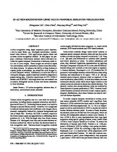
sification in a nearest neighbour fashion. In the same way, Lui et al. [22]
137
factorize raw pixel from images by high-order singular value decomposition
138
in order to represent the actions on Stiefel and Grassmann manifolds. How-
139
ever, in this work where raw pixels are directly factorized as manifold points,
140
there is no dynamic modelling of the sequence. In addition, only distances
141
obtained between all tangent vectors are used for action classification and
142
there is no training process on data.
143
Kernels [23, 24] are also used in order to transform subspaces of a man-
144
ifold onto a space where Euclidean metric can be applied. Shirazi et al.
145
[23] embed Grassmann manifolds upon a Hilbert space to minimize cluster-
146
ing distortions and then apply a locally discriminant analysis using a graph.
147
Video action classification is then obtained by a Nearest-Neighbour classi-
148
fier applied on Euclidean distances computed on the graph-embedded kernel.
149
Similarly, Harandi et al. [24] propose to represent the spatio-temporal as-
150
pect of the action by subspaces elements of a Grassmann manifold. Then,
151
they embed this manifold into reproducing kernel of Hilbert spaces in order
152
to tackle the problem of action classification on such manifolds. Gall et al.
153
[25] use multi-view system coupling action recognition on 2D images with
154
3D pose estimation, were the action-specific manifolds are acting as a link
8
155
between them.
156
All these approaches cited above are based on features extracted from
157
2D video sequences as silhouettes or raw pixels from images. However, the
158
recent emergence of low-cost depth sensors opens the possibility of revisiting
159
the problem of activity modelling and learning using depth data-driven.
160
2.2. Depth data-driven approaches
161
Maps obtained by depth sensors are able to provide additional body shape
162
information to di↵erentiate actions that have similar 2D projections from a
163
single view. It has therefore motivated recent research works, to investigate
164
action recognition using the 3D information. Recent surveys [26, 27] are re-
165
porting works on depth videos. First methods used for activity recognition
166
from depth sequences have tendency to extrapolate techniques already de-
167
veloped for 2D video sequences. These approaches use points in depth map
168
sequences as a gray pixels in images to extract meaningful spatiotemporal
169
descriptors. In Wanqing et al. [28], depth maps are projected onto the three
170
orthogonal Cartesian planes (X
171
contours of the projections are sampled for each frame. The sampled points
172
are used as bag-of-points to characterize a set of salient postures that corre-
173
spond to the nodes of an action graph used to model explicitly the dynamics
174
of the actions. Local feature extraction approaches like spatiotemporal inter-
175
est points (STIP) are also employed for action recognition on depth videos.
176
Bingbing et al.[29] use depth maps to extract STIP and encode Motion His-
177
tory Image (MHI) in a framework combining color and depth information.
178
Xia et al [30] propose a method to extract STIP a on depth videos (DSTIP).
179
Then around these points of interest they build a depth cuboid similarity
Y, Z
9
X, and Z
Y planes) and the
180
feature as descriptor for each action. In the work proposed by Vieira et al.
181
[31], each depth map sequence is represented as a 4D grid by dividing the
182
space and time axes into multiple segments in order to extract SpatioTempo-
183
ral Occupancy Pattern features (STOP). Also in Wang et al. [32], the action
184
sequence is considered as a 4D shape but Random Occupancy Pattern (ROP)
185
is used for features extraction. Yang et al.[33] employ Histograms of Oriented
186
Gradients features (HOG) computed from Depth Motion Maps (DMM), as
187
the representation of an action sequence. These histograms are then used as
188
input to SVM classifier. Similarly, Oreifej et al. [34] compute a 4D histogram
189
over depth, time, and spatial coordinates capturing the distribution of the
190
surface normal orientation. This histogram is created using 4D projectors
191
allowing quantification in 4D space.
192
The availability of 3D sensors has recently made possible to estimate 3D
193
positions of body joints. Especially thanks to the work of Shotton et al.
194
[6], where a real-time method is proposed to accurately predict 3D positions
195
of body joints. Thanks to this work, skeleton based methods have become
196
popular and many approaches in the literature propose to model the dynamic
197
of the action using these features.
198
Xia et al. [35] compute histograms of the locations of 12 3D joints as a
199
compact representation of postures and use them to construct posture visual
200
words of actions. The temporal evolutions of those visual words are modeled
201
by a discrete HMM. Yang et al. [36] extract three features, as pair-wise dif-
202
ferences of joint positions, for each skeleton joint. Then, principal component
203
analysis (PCA) is used to reduce redundancy and noise from feature, and it
204
is also used to obtain a compact Eigen Joints representation for each frame.
10
205
Finally, a na¨ıve-Bayes nearest-neighbour classifier is used for multi-class ac-
206
tion classification. The popular Dynamic Time Warping (DTW) technique
207
[37], well-known in speech recognition area, is also used for gesture and action
208
recognition using depth data. The classical DTW algorithm was defined to
209
match temporal distortions between two data trajectories, by finding an op-
210
timal warping path between the two time series. The feature vector of time
211
series is directly constructed from human body joint orientation extracted
212
from depth camera or 3D Motion Capture sensors. Reyes et al. [38] per-
213
form DTW on a feature vector defined by 15 joints on a 3D human skeleton
214
obtained using PrimeSense NiTE. Similarly, Sempena et al. [39], by the 3D
215
human skeleton model, use quaternions to form a 60-element feature vec-
216
tor. The obtained warping path, by classical DTW algorithm, between two
217
time series is mainly subjected to some constraints: (1) boundary constraint
218
which enforces the first elements of the sequences as well as the last one
219
to be aligned to each other (2) monotonicity constraint which requires that
220
the points in the warping path are monotonically spaced in time in the two
221
sequences. This technique is relatively sensitive to noise as it requires all
222
elements of the sequences to be matched to a corresponding elements of the
223
other sequence. It also has a drawback related to its computational complex-
224
ity incurring in quadratic cost. However, many works have been proposed to
225
bypass its drawbacks by means of probabilistic models [40] or incorporating
226
manifold learning approach [17, 16].
227
Recent research has carried on more complex challenge of in-line recogni-
228
tion systems for di↵erent applications, in which a trade-o↵ between accuracy
229
and latency can be highlighted. Ellis et al. [41] study this trade-o↵ and
11
230
employed a Latency Aware Learning (LAL) method, reducing latency when
231
recognizing actions. They train a logistic regression-based classifier, on 3D
232
joint position sequences captured by kinect camera, to search a single canon-
233
ical posture for recognition. Another work is presented by Barnachon et
234
al. [42], where a histogram-based formulation is introduced for recognizing
235
streams of poses. In this representation, classical histogram is extended to
236
integral one to overcome the lack of temporal information in histograms.
237
They also prove the possibility of recognizing actions even before they are
238
completed using the integral histogram approach. Tests are made on both 3D
239
MoCap from TUM kitchen dataset [43] and RGB-D data from MSR-Action
240
dataset [28].
241
Some hybrid approaches combining both skeleton data features and depth
242
information were recently introduced, trying to combine positive aspects of
243
both approaches. Azary et al. [44] propose spatiotemporal descriptors as
244
time-invariant action surfaces, combining image features extracted using ra-
245
dial distance measures and 3D joint tracking. Wang et al. [45] compute
246
local features on patches around joints for human body representation. The
247
temporal structure of each joint in the sequence is represented through a tem-
248
poral pattern representation called Fourier Temporal Pyramid. In Oreifej et
249
al. [34], a spatiotemporal histogram (HON4D) computed over depth, time,
250
and spatial coordinates is used to encode the distribution of the surface nor-
251
mal orientation. Similarly to Wang et al. [45], HON4D histograms [34] are
252
computed around joints to provide the input of an SVM classifier. Althloothi
253
et al. [46] represent 3D shape features based on spherical harmonics repre-
254
sentation and 3D motion features using kinematic structure from skeleton.
12
255
Both feature are then merged using multi kernel learning method.
256
It is important to note that, to date, few works have very recently pro-
257
posed to use manifold analysis for 3D action recognition. Devanne et al. [47],
258
propose a spatiotemporal motion representation to characterize the action as
259
a trajectory which corresponds to a point on Riemannian manifold of open
260
curves shape space. These motion trajectories are extracted from 3D joints,
261
and the action recognition is performed by K-Nearest-Neighbor method ap-
262
plied on geodesic distances obtained on open curve shape space. Azary et al.
263
[48] use a Grassmannian representation as an interpretation of depth motion
264
image (DMI) computed from depth pixel values. All DMI in the sequence
265
are combined to create a motion depth surface representing the action as a
266
spatiotemporal descriptor.
267
2.3. Contributions and proposed approach
268
On the one hand, approaches modelling actions as elements of manifolds
269
[49, 50, 9] prove that it is an appropriate way to represent and compare
270
videos. On the other hand, very few works deal with this task using depth
271
images and it is still possible to improve learning step using these models.
272
Besides, linear dynamic systems [51] show more and more promising results
273
on the motion modelling since they exhibit the stationary properties in time,
274
so they fit for action representation.
275
In this paper, we propose the use of geometric structure inherent in the
276
Grassmann manifold for action analysis. We perform action recognition by
277
introducing a manifold learning algorithm in conjunction with dynamic mod-
278
elling process. In particular, after modelling motions as a linear dynamic sys-
279
tems using ARMA models, we are interested in a representation of each point 13
280
on the manifold incorporating class separation properties. Our representa-
281
tion takes benefit of statistics in the Grassmann manifold and action classes
282
representations on tangent spaces. From spatiotemporal point of view, each
283
action sequence is represented in our approach as linear dynamical system
284
acquiring the time series of 3D joint-trajectory. From geometrical point of
285
view, each action sequence is viewed as a point on the Grassmann manifold.
286
In terms of machine learning, a discriminative representation is provided for
287
each action thanks to a set of appropriate tangent vectors taking benefit
288
of manifold proprieties. Finally, the efficiency of the proposed approach is
289
demonstrated on three challenging action recognition datasets captured by
290
depth cameras.
291
3. Spatiotemporal modelling of action
292
The human body can be represented as an articulated system composed
293
of hierarchical joints that are connected with bones, forming a skeleton. The
294
two best-known skeletons provided by the Microsoft Kinect sensor, are those
295
obtained by official Microsoft SDK, which contains 20 joints, and PrimeSense
296
NiTE which contains only 15 joints (see Figure 2). The various joint con-
297
figurations throughout the motion sequence produce a time series of skeletal
298
poses giving the skeleton movement. In our approach, an action is simply
299
described as a collection of time series of 3D positions of the joints in the
300
hierarchical configuration.
301
3.1. Linear dynamic model
302
Let pjt denote the 3D position of a joint j at a given frame t i.e., pj =
303
[xj , y j , z j ]j=1:J , with J is the number of joints. The joint position time-series 14
1
1 2
13
15
19
17
14
13
18
4 5
16
20
3
20
6
5
6
7 7
14
2
16
3
19
15
8
8
9
10
12
11
12
11
(a)
(b)
Figure 2: Skeleton joint locations captured by Microsof Kinect sensor (a) using Microsoft SDK (b) using PrimeSense NiTE. Joint signification are: (1) head (2) shoulder center (3) spine (4) hip center (5/6) left/right hip (7/8) left/ ight knee (9/10) left/right ankle (11/12) left/right foot (13/14) left/right shoulder (15/16) left/right elbow (17/19) left/right wrist (19/20) left/right hand.
304
of joint j is pjt = {xjt , ytj , ztj }t=1:T j=1:J , with T the number of frames. A motion
305
sequence can then be seen as a matrix collecting all time-series from J joints,
306
i.e., M = [p1 p2 · · · pT ], p 2 R3⇤J .
307
At this level, we could consider using DTW algorithm [37] to find optimal
308
non-linear warping function to match these given time-series as proposed by
309
[38, 39, 16]. However, we opted for a system combining a linear dynamic
310
modelling with statistical analysis on a manifold, avoiding the boundary and
311
the monotonicity constraints presented by classical DTW algorithm. Such a
312
system is also less sensitive to noise due to the poor estimation of the joint
313
locations, in addition to its reduced computational complexity.
314
The dynamic and the continuity of movement imply that the action can
315
not be resumed as a simply set of skeletal poses because of the temporal 15
316
information contained in the sequence. Instead of directly using original
317
joint position time-series data, we believe that a linear dynamic system, like
318
that often used for dynamic texture modelling, is essential before manifold
319
analysis. Therefore, to capture both the spatial and the temporal dynamics
320
of a motion, linear dynamical system characterized by ARMA models are
321
applied to the 3D joint position time-series matrix M .
322
323
The dynamic captured by the ARMA [52, 53] model during an action sequence M can be represented as: p(t) = Cz(t) + w(t),
w(t) ⇠ N (0, R),
z(t + 1) = Az(t) + v(t), 324
v(t) ⇠ N (0, Q)
(1)
where z 2 Rd is a hidden state vector, A 2 Rd⇥d is the transition matrix
325
and C 2 R3⇤J⇥d is the measurement matrix. w and v are noise components
326
modeled as normal with mean equal to zero and covariance matrix R 2
327
328
329
330
331
332
R3⇤J⇥3⇤J and Q 2 Rd⇥d respectively. The goal is to learn parameters of the P model (A, C) given by these equations. Let U V T be the singular value decomposition of the matrix M . Then, the estimated model parameters A P T P 1 and C are given by: Cˆ = U and Aˆ = V D1 V (V T D2 V ) 1 , where D1 = [0 0, I⌧ size ⌧
1
0], D2 = [I⌧
1
0, 0 0] and I⌧
1
is the identity matrix of
1.
333
Comparing two ARMA models can be done by simply comparing their
334
observability matrices. The expected observation sequence generated by an
335
ARMA model (A,C) lies in the column space of the extended observability
336
T matrix given by ✓1 = [C T , (CA)T , (CA2 )T , ...]T . This can be approximated
337
T by the finite observability matrix ✓m = [C T , (CA)T , (CA2 )T , ..., (CA2 )m ]T
16
338
[18]. The subspace spanned by columns of this finite observability matrix
339
corresponds to a point on a Grassmann manifold.
340
3.2. Grassmann manifold interpretation
341
Grassmannian analysis provides a natural way to deal with the problem of
342
sequence matching. Especially, this manifold allows to represent a sequence
343
by a point on its space and o↵ers tools to compare and to do statistics on
344
this manifold. The classification problem of sets of motions represented by a
345
collection of features can be transformed to point classification problem on
346
the Grassmann manifold.
347
In this work we are interested in Grassmann manifolds which definition
348
is as below.
349
Definition: The Grassmann manifold Gn⇥d is a quotient space of orthogonal
350
group O(n) and is defined as the set of d-dimensional linear subspaces of Rn .
351
Points on the Grassmann manifold are equivalent classes of n ⇥ d orthogonal
352
matrices, with d < n, where two matrices are equivalent if their columns span
353
the same d-dimensional subspace.
354
Let µ denotes an element on Gn⇥d , the tangent space to this element Tµ on
355
Gn,d is the tangent plane to the surface of the manifold at µ. It is possible
356
to map a point U , of the Grassmann manifold, to a vector in the tangent
357
space Tµ using the logarithm map as defined by Turaga et al. [18]. An other
358
important tool in statistics is the exponential map Expµ : Tµ (Gn,d ) ! Gn,d ,
359
which allows to move on the manifold.
360
Two points U1 and U2 on Gn,d are equivalent if one can be mapped into
361
the other one by d ⇥ d orthogonal matrix [54]. In other words, U1 and U2 are
362
equivalent if the d columns of U1 are rotations of U2 . The minimum length 17
363
curve connecting these two points is the geodesic between them computed
364
as: dgeod (U1 , U2 ) =k [✓1 , ✓2 , · · · , ✓i , · · · , ✓d ] k2
(2)
365
where ✓i is the principal angle vector which can be computed through the
366
SVD of U1T U2 .
367
4. Learning process on the manifold
368
Let {U1 , · · · UN } be N actions represented by points on the Grassmann
369
manifold. A common learning approach on manifolds is based on the use
370
of only one-tangent space, which usually can be obtained as the tangent
371
space to the mean (µ) of the entire data points {Ui }i=1:N without regard
372
to class labels. All data points on the manifold are then projected on this
373
tangent space to provide the input of a classifier. This assumption provide an
374
accommodated solution to use a classical supervised learning on the manifold.
375
However, this flattening of the manifold through tangent space is not efficient
376
since the tangent space on the global mean can be far from other points.
377
A more appropriate way is to consider separate tangent spaces for each
378
class at the class-mean. The classification is then performed in these indi-
379
vidual tangent spaces as in [18].
380
Some other approaches explore the idea of tangent bundle as in Lui et
381
al. [21, 22], in which all tangent planes of all data points on the manifold
382
are considered. Tangent vectors are then computed between all points on
383
a Grassmann manifold and action classification is performed thanks to ob-
384
tained distances.
385
We believe that using several tangent spaces, obtained for each class of 18
386
the training data points, is more intuitive. However, the question here is how
387
to learn a classifier in this case?
388
In the rest of the section, we present a statistical computation of the mean
389
in the Grassmann manifold [55]. Then, we propose two learning methods on
390
this manifold taking benefit from tangent space class specific and tangent
391
bundle [21]: Truncated Wrapped Gaussian (TWG) [56] and Local Tangent
392
Bundle SVM (LBTSVM).
393
4.1. Mean computation on the Grassmann manifold
394
The Karcher mean [55] enables computation of a mean representative for
395
a cluster of points on the manifold. This mean should belong to the same
396
space as the given points. In our case, we need Karcher mean to compute
397
averages on the Grassman manifold and more precisely means of each action
398
class which represents the action at best. The algorithm exploits log and exp
399
maps in a predictor/corrector loop until convergence to an expected point.
400
The computation of a mean can be used to perform an action classification
401
solution. This can be done by a s simple comparison of an unknown action,
402
represented as a point on the manifold, to all class-means and assigning it to
403
the nearest one using the distance presented in Equation 2.
404
4.2. Truncated Wrapped Gaussian
405
In addition to the mean µ computed by Karcher mean on {Ui }i=1:N , we
406
look for the standard deviation value
between all actions in each class of
407
training data. The
408
are the projections of actions from the Grassmann manifold into the tangent
must be computed on {Vi }i=1:N where V = expµ 1 (Ui )
19
409
space defined on the mean µ. The key idea here is to use the fact that the
410
tangent space Tµ (Gn,d ) is a vector space.
411
Thus, we can estimate the parameters of a probability density function
412
such as a Gaussian and then use the exponential map to wrap these param-
413
eters back onto the manifold using exponential map operator [18]. However,
414
the exponential map is not a bijection for the Grassmann manifold. In fact, a
415
line on tangent space, with infinite length, can be warpped around the man-
416
ifold many times. Thus, some points of this line are going to have more than
417
one image on Gn,d . It becomes a bijection only if the domain is restricted.
418
Therefore, we can restrict the tangent space by a truncation beyond a radius
419
of ⇡ in Tµ (Gn,d ). By truncation, the normalization constant changes for mul-
420
tivariate density in Tµ (Gn,d ). In fact, it gets scaled down depending on how
421
much of the probability mass is left out of the truncation region.
422
423
Let f (x) denotes the probability density function (pdf) defined on Tµ (Gn,d ) by : f (x) = p
424
1 2⇡
2
e2
x2 2
After truncation, an approximation of f gives: f (x) ⇥ 1|x|