Accurate Approximation of Invariant Zeros For a Class ...

Accurate Approximation of Invariant Zeros For a Class of SISO Abstract Boundary Control Systems Ada Cheng Department of Science and Mathematics Kettering University Flint, Michigan, USA [email protected]

Abstract— Low order accurate finite dimensional approximation of an infinite dimensional system is important in controller design. In this paper, we introduce a new method to accurately compute the zeros.

I. INTRODUCTION The zeros of a system transfer function are important in controller design. For instance, the presence of right-handplane zeros restricts the achievable sensitivity reduction. The presence of right-hand-plane zeros also makes the use of an adaptive controller impractical in most situations. Furthermore, if a zero is close to a pole, the system is close to being non-minimal and hence uncontrollable and/or unobservable e.g. [5, sect. 2.5]. It is also difficult to obtain robust stability for these systems [5, sect. 2.5]. Systems modeled by partial differential equations with boundary control arise in many applications; for instance heating processes, active noise control and flexible structures. Typically a finite-dimensional approximation is used for simulation and also for controller design. One common approximating scheme is the finite element method (FEM). In general, a finite-element approximation provides good estimates of the exact system eigenvalues and hence of the poles of the transfer function. As illustrated below a finite-element approximation may approximate the zeros of a system very poorly. In [4] it was shown that modal truncations of a controlled beam example yield inaccurate calculations of the system zeros. In particular, right-hand plane zeros appear in certain modal truncations that are not present in the original infinite-dimensional model. We found modal approximations to have similar problems for an example we give here. Here, we introduce a different approach, that we call the direct method, for calculation of the system zeros. The zeros are obtained by computing the eigenvalues of an approximation to a related system with zero output. This technique has two advantages. First, the computed zeros are more accurate since most numerical methods accurately approximate eigenvalues. Secondly, the zeros of the system are simply the eigenvalues of some matrix. These can be computed very efficiently. We illustrate our technique with collocated and non-collocated control of a heated rod.

Kirsten Morris Department of Applied Mathematics University of Waterloo Waterloo, Ontario, CANADA. [email protected]

II. D IRECT M ETHOD TO C ALCULATE Z EROS In this paper we consider boundary control systems as defined in [7]:  d z(0) = z0  dt z(t) = ∆z, (1) Γz(t) = u(t),  y(t) = Cz(t). The operators ∆ ∈ L(Z, H), Γ ∈ L(Z, U) and C ∈ L(Z, Y). The spaces (Z, k · kZ ), (H, k · kH ), (U, k · kU ), (Y, k · kY ) are all Hilbert spaces. The spaces (U, k · kU ), (Y, k · kY ) are the input and output space respectively. In this paper we consider only SISO systems: U = Y = R. The space Z is a dense subspace of H with continuous, injective embedding ιZ . The triple (∆, Γ, C) refers to a boundary control system as above. We will assume that a boundary control system satisfies the standard assumptions as in [3], [7]. Any such system can be put into a state-space form [7]. We will not do so here. Note however that the operator C above is not in general the observation operator in the state-space formulation. We now obtain a representation of the transfer function of a boundary control system. The transfer function is defined in terms of an abstract elliptic problem associated with the boundary control system. Definition 2.1: The abstract elliptic problem (∆, Γ)e corresponding to the boundary control system (∆, Γ),as defined in (1), is ¾ ∆z = sz, s∈C (2) Γz = u(s). We denote the solution z ∈ Z by z(s). Let α denote the growth bound of the semigroup associated with ∆. The abstract elliptic problem (2) has a unique solution z(s) for all u and Re s > α [7, 2.20]. The system transfer function may be described through the solutions to the abstract elliptic problem (2). Theorem 2.2: (For proof, see[3]) Let (∆, Γ, C) define a boundary control system. Then there exists a real number α such that the transfer function, G(s), of the boundary control system (∆, Γ, C) is given by G(s)u(s) = Cz(s) ∀s ∈ C, with Re(s) > α,

(3)

where z(s) is the solution to the abstract elliptic problem (2) with input u(s).

Definition 2.3: The transmission zeros of (1) is the set of all s such that G(s) = 0.

III. E XAMPLE : O NE D IMENSIONAL H EAT E QUATION W ITH N EUMANN B OUNDARY C ONTROL

We define invariant zeros through the boundary control system description. This definition is consistent with that in [2] for the zero dynamics of a SISO system with collocated observation and control.

Consider the one-dimensional heat equation with Neumann boundary control at the right end:  ∂2z ∂z   = , x ∈ [0, 1]   ∂t ∂x2    z(x, 0) = 0,   ∂z (5) (0, t) = 0,  ∂x   ∂z    (1, t) = u(t),   ∂x  y(t) = z(x1 , t), x1 ∈ [0, 1].

Definition 2.4: The invariant zeros of (1) are λ ∈ C such that there is a non-trivial solution z ∈ Z to the constrained zero system λz Cz

= ∆z, = 0.

¾ (4)

The transmission zeros of a system have a relationship to the invariant zeros that is entirely analogous to the relationship between the transfer function poles and the eigenvalues in the state-space description of a system. Theorem 2.5: Every transmission zero is an invariant zero. Also, any invariant zero that is not in the spectrum of A where Az = ∆z with D(A) = {z ∈ Z | Γz = 0} is a transmission zero. Proof: Suppose that λ ∈ ρ(A) is an invariant zero, and let zo be the corresponding element of Z. Since λ ∈ ρ(A), Γzo 6= 0. Define uo = Γzo . We have

The transfer function is

√ cosh( sx1 ) √ . G(s) = √ s sinh( s)

(6)

Two Galerkin approximations were used: a finite-element (FEM) approximation with linear splines and also a modal approximation using the eigenfunctions as a basis. The constrained zero system is  ∂2z  λz = , x ∈ [0, 1]    ∂x2 ∂z (7) (0) = 0,    ∂x  z(x1 ) = 0. Note that the constrained zero system involves a boundary value problem to be solved on [0, x1 ].

∆zo Γzo Czo

= λzo , = uo = 0.

Since λ ∈ ρ(A), it is not a pole of the transfer function G(s), and by comparing to (2), we see that G(λ) = 0. Now suppose that G(λ) = 0 for some λ. Let zo be the solution to the (2, 3) with s = λ and u = 1. Substituting into (4) we obtain that λ is an invariant zero. ¤ Our method is to apply a standard numerical method (we choose finite element with linear splines) to the constrained zero system (4) to obtain a finite-dimensional approximation, λzn = AN zn where Czn = 0. The zeros of the original infinite dimensional system, are approximated by the eigenvalues of AN . This we will call the direct method. In the next section we shall compare the zeros calculated using our direct method to those computed as the invariant zeros of standard finite-dimensional approximations. Invariant zeros are calculated as the solution to a generalized eigenvalue problem. Eigenvalue calculation is a built-in function in many standard software packages, such as MATLAB. Working within a standard package, the eigenvalue calculation is much quicker than the calculation of the invariant zeros.

A. Case 1: Collocated Observation If x1 = 1 in Equation (5) then the zeros of G(s) are zn = − 41 (2n + 1)2 π 2 . We first consider a FEM approximation, with evenly spaced linear splines. The zeros of the 15 element approximation are shown in Figure 1. We see that the approximate zeros from both FEM and our direct method are identical and are reasonably close to the exact zeros of the system. We also used a modal approximation using the eigenfunctions, φk (x) = cos(kπx), as a basis. The modal approximations also give acceptable results. B. Case 2: Non-Collocated Observation If x1 = 0 then there are no transmission zeros. If x1 ∈ (0, 1), then the zeros of G(s) are zn = − 4x1 1 (2n + 1)2 π 2 . All zeros are in the left-hand-plane. We will now show a stronger result, that the stable part of the transfer function (6) is outer (or minimum-phase). Theorem 3.1: The function √ cosh( sx1 ) √ √ G(s) = s sinh( s) where 0 ≤ x1 ≤ 1 has a factorization 1 g(s) s where g(s) is an outer function in H∞ . G(s) =

Zeros of 1-D Heat with Neumann BC and N=15

Zeros of 1-D Heat with Neumann BC and N=15 400 1 300

200 0.5 100

0

0

-100

-200

-0.5

-1

-300

Exact Zeros FEM Zeros Modal Zeros Direct Zeros -2500

Fig. 1.

Exact Zeros FEM Zeros Modal Zeros Direct Zeros

-400 -2000

-1500

-1000

-500

-25000

0

Zeros Estimates for 1-D heat with x1 = 1 and N = 15.

Proof: Define g(s) = sG(s). It is straightforward to show that g(s) ∈ H∞ for 0 ≤ x1 ≤ 1. It remains to show that g is outer. Since g ∈ H∞ , it can be associated with an operator Γg : H2 → H2 defined by Γg f = gf. It will be shown that the range of Γg is dense in H2 and hence by definition, g is outer. If x1 = 1 then g(s)−1 ∈ H∞ and the result is trivial. For other values of x1 the following approach shows that g is outer. The function z sinh z is entire, √ with a Taylor expansion √ involving only z 2 . It follows that s sinh( s) is entire. It has a product expansion i.e. [1, Eg 9.5.3] √ ∞ ³ Y sinh( s) s ´ √ = 1+ 2 2 . (8) n π s n=1 This series is uniformly convergent on compact subsets of the complex plane. Define the sequence of functions fN ∈ H∞ N ³ Y

s ´ 1+ 2 2 n π √ . fN (s) = n=1 cosh( sx1 )

Fig. 2.

-20000

-15000

kguN − yk2 = 0 with uN = fN y can be made arbitrarily small by choosing N large enough.

-5000

Zeros Estimates for 1-D heat with x1 =

1 3

0

and N = 15.

For any ² > 0, choose R > π 2 so that 1 ²2 F (R, y) < . 2π 16 where

Z

∞

F (R, y) = sup x>0

(9) Z

|y(x+jω)|2 dω−sup x>0

−∞

R

|y(x+jω)|2 dω.

−R

We now show that gfN − 1 is uniformly bounded in N for |s| > R, Res > 0. First, note that ! Ã 1 ¡ ¢ −1 . gfN − 1 = Q∞ s n=N +1 1 + n2 π 2 For |s| > R > π 2 , and Res > 0, ¯ ¯ 1 ¯ ¡ ¯ Q∞ ¯ n=N +1 1 + ≤

Q∞ n=N +1

≤

Q∞ n=N +1

Choose any y ∈ H2 and let k · k2 indicates the H2 -norm. It will be proven that g is outer by showing that

-10000

≤

≤
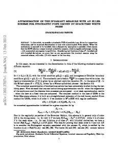
0 R ! Z −R ²2 2 + sup |(guN − y)(x + jω)| dω < . (13) 4 x>0 −∞ Since the product expansion (8) converges uniformly on compact sets and √ sinh s √ > 0, inf Res>0 s we can choose N large enough that sup |gfN (s) − 1| < |s| 0 were arbitrary, it follows that the range of Γg is dense in H2 , and so g is an outer function. ¤ For numerical computation, we choose x1 = 13 . As in the collocated case, we calculated the invariant zeros of a finiteelement approximation (linear splines) and also of a modal approximation. The calculated zeros are shown in Figure 2 5. The order of all approximations is 15. As can be seen in Figure 3 and 4, both FEM and modal approximations produce right half plane zeros. The direct method (see Figure 5 did not produce any right half plane zeros. Thus, although the

Fig. 4.

Zeros Estimates for 1-D heat with x1 =

1 3

and N = 15. (Modal)

exact transfer function is 1s g(s) where g is an outer function, the approximations contain a non-trival outer part. This may lead to misleading results in controller design, particularly when using H∞ methods. IV. C ONCLUSION In this paper, we presented a new method for improving the accuracy and speed for computing zeros of infinitedimensional systems. This direct method was illustrated with several simple examples. Our preliminary findings are encouraging. Future work will involve developing this method for problems with more than one space dimension. This technique may be useful for approximating multidimensional systems. Usually for these system a high order state-space approximation is necessary. Typically the number of inputs and outputs is relatively low. A low order approximation may possibly be obtained by using the zeros and poles. V. REFERENCES [1] M. Y. Antimirov, A.A. Kolyshkin and R. Vaillancourt, Complex Variables, Academic Press, 1998. [2] C.I. Byrnes, D.S. Gilliam and J. He, “Root-locus and boundary feedback design for a class of distributed parameter systems”, SIAM Jour. on Control and Optimization, Vol. 32, no. 5, pg. 1364-1427, 1994. [3] A. Cheng and K.A. Morris, ”Well-Posedness of Boundary Control Systems”, SIAM Jour. on Control and Optimization, Vol. 42, no. 4, pg. 1244-1265, 2003.

Transmission zeros of 1-D Heat with Neumann BC and N=15 (zoomed in) 10

5

0

-5

Direct Zeros Exact Zeros -10 -6000

-5000

-4000

-3000

-2000

-1000

0

Direct Zeros

Fig. 5. Zeros Estimates for 1-D heat with x1 = zoomed in.)

1 3

and N = 15. (Direct,

[4] D.K. Lindner, K.M. Reichard and L.M. Tarkenton, ”Zeros of Modal Models of Flexible Structures”. IEEE Trans. on Auto. Control, Vol. 38, No. 9, pg. 1384-1388, 1993. [5] K.A. Morris, Introduction to Feedback Control, Academic Press, 2001. [6] K.A. Morris, ”Noise Reduction in Ducts Achievable by Point Control”, Transactions of the ASME, Vol 120, pp 216-223, 1998. [7] D. Salamon, ”Infinite-dimensional linear systems with unbounded control and observation: A functional analytic approach”, Transactions of the American Mathematical Society, Vol. 300, pg. 383–431, 1987.