(BEM) which discretize the surface of the iron yoke and Finite Elements (FEM) for the mod- ... calcula-tion of the magnetization (reduced field) of the yoke.
EUROPEAN ORGANIZATION FOR NUCLEAR RESEARCH European Laboratory for Particle Physics
Large Hadron Collider Project
LHC Project Report 284
Accurate Calculation of Magnetic Fields in the End Regions of Superconducting Accelerator Magnets using the BEM-FEM Coupling Method S. Kurz1 and S. Russenschuck2
Abstract In this paper a new technique for the accurate calculation of magnetic fields in the end regions of superconducting accelerator magnets is presented. This method couples Boundary Elements (BEM) which discretize the surface of the iron yoke and Finite Elements (FEM) for the modelling of the nonlinear interior of the yoke. The BEM-FEM method is therefore specially suited for the calculation of 3-dimensional effects in the magnets, as the coils and the air regions do not have to be represented in the finite-element mesh and discretization errors only influence the calcula-tion of the magnetization (reduced field) of the yoke. The method has been recently implemented into the CERN-ROXIE program package for the design and optimization of the LHC magnets. The field shape and multipole errors in the two-in-one LHC dipoles with its coil ends sticking out of the common iron yoke is presented.
1 2
ITE, University of Stuttgart, Germany CERN, Geneva, Switzerland (LHC Division)
Presented at the 1999 Particle Accelerator Conference, March 29 – April 2, 1999, New York, USA
Administrative Secretariat LHC Division CERN CH - 1211 Geneva 23 Switzerland Geneva, 23 April 1999
Accurate Calculation of Magnetic Fields in the End Regions of Superconducting Accelerator Magnets Using the BEM-FEM Coupling Method S. Kurz∗ , S. Russenschuck ∗ ITE, University of Stuttgart, Germany CERN, Geneva, Switzerland Abstract In this paper a new technique for the accurate calculation of magnetic fields in the end regions of superconducting accelerator magnets is presented. This method couples Boundary Elements (BEM) which discretize the surface of the iron yoke and Finite Elements (FEM) for the modelling of the nonlinear interior of the yoke. The BEM-FEM method is therefore specially suited for the calculation of 3dimensional effects in the magnets, as the coils and the air regions do not have to be represented in the finite-element mesh and discretization errors only influence the calculation of the magnetization (reduced field) of the yoke. The method has been recently implemented into the CERNROXIE program package for the design and optimization of the LHC magnets. The field shape and multipole errors in the two-in-one LHC dipoles with its coil ends sticking out of the common iron yoke is presented.
1
INTRODUCTION
The design and optimization of the LHC magnets is dominated by the requirement of an extremely uniform field which is mainly defined by the layout of the superconducting coils. Even very small geometrical effects such as the insufficient keystoning of the cable, the insulation, grading of the current density in the cable due to different cable compaction and coil deformations due to collaring, cool down and electromagnetic forces have to be considered for the field calculation. In particular for the 3D case, commercial software has proven to be hardly appropriate for the field optimization of the LHC magnets. Therefore the ROXIE program package was developed at CERN for the design and optimization of the LHC superconducting magnets. Using the BEM-FEM coupling method [1] yields the reduced field in the aperture due to the magnetization of the iron yoke and avoids the representation of the coil in the FE-meshes.
2
This approach has the following intrinsic advantages: (1) The coil field can be taken into account in terms of its ~ S , which can be obtained easily source vector potential A from the filamentary currents IS by means of Biot-Savart type integrals without meshing of the coil. (2) The BEMFEM coupling method allows for the direct computation of ~ R rather than the total vecthe reduced vector potential A ~ Then numerical errors do not influence tor potential A. ~ S due to the superconducting the dominating contribution A coil. (3) The surrounding air region needs not to be meshed at all. This simplifies the preprocessing and avoids artificial boundary conditions at some ”far” boundaries. Moreover, the geometry of the permeable parts can be modified without taking care of the mesh in the surrounding air region. This strongly supports the feature based, parametric geometry modelling which is required for mathematical optimization. When the BEM-FEM coupling method is applied, only the magnetic sub-domain Ωi which coincides with the magnetic yoke has to be discretized by finite elements. Iron saturation effects can then be dealt with within the finite element framework. The nonmagnetic sub-domain Ωa which represents the surrounding air region and the excitation coil is treated by the boundary element method. Only the common boundary Γ needs to be discretized by boundary el~ S can be obtained ements. The source vector potential A from the filamentary current IS by means of the Biot-Savart type integral I ~ S = µ0 IS u∗ d~l. (2) A C
In (2), the Green’s function u∗ is the fundamental solution of the Laplace equation, which is in 2D u∗ = −
~ R. ~=A ~S + A A
(1)
(3)
and in 3D
THE BEM-FEM COUPLING METHOD
~ in a certain point ξ~ in the The total magnetic induction B aperture of the magnet can be decomposed into a contribu~ S due to the superconducting coil and a contribution tion B ~ BR due to the magnetic yoke. If the fields are expressed in ~ = curl A, ~ then the terms of the magnetic vector potential B decomposition into source and reduced contributions gives
1 ~ ln |~x − ξ| 2π
u∗ =
1 ~ 4π|~x − ξ|
.
(4)
~ S and ~x is the integration point ξ~ is the evaluation point of A on C.
2.1
The FEM part
Inside the magnetic domain Ωi a gauged vector-potential formulation is applied. With Maxwell’s equations
~ = J~ and div B ~ = 0 for magnetostatic problems, curlH the constitutive equation ~ = µ(H) ~ ·H ~ = µ0 (H ~ +M ~) B
(5)
~ = curl A ~ we get and the vector-potential formulation B 1 ~ = J~ + curlM ~. curlcurlA µ0
(6)
~ the weak forIntroducing the penalty term −grad µ10 divA mulation reads Z 1 ~ + divwdiv ~ dΩi (curlw ~ · curlA ~ A) µ0 Ωi � � I 1 1 ~ ~ curlA × ~n − − w ~· (divA)~n dΓai µ0 µ0 Γai Z Z ~ − w ~ · J~ dΩi (7) M · curlw ~ dΩi = Ωi
Ωi
which can be transformed to Z 1 ~ · ~ea ) · gradwa dΩi grad(A µ0 Ωi ! I ~ 1 ∂A ~ × ~ni ) · w − − (µ0 M ~ a dΓai = µ0 Γai ∂ni Z Z ~ w ~ a · J~ dΩi M · curlw ~ a dΩi + Ωi
(8)
(9)
~ BEM ∂A Γai ∂na
By definition the BEM domain Ωa does not contain any ~ = 0 and µ = µ0 . One more integration iron and therefore M by parts of the weak integral form (8) and choosing the Cartesian components of the vector weighting function as the fundamental solution of the Laplace equation yields I I Θ ~ ~ Γai u∗ dΓai + A ~ Γai q ∗ dΓai A+ Q 4π Γai Γai Z ~ ∗ dΩa = µ0 Ju (13) ∂u with the abbreviation q ∗ = ∂n . The right hand side of a Eq. (13) is a Biot-Savart type integral for the source vec~ at any arbitrary ~ s . The vector potential A tor potential A point ~r0 ∈ Ωa can be computed from (13) once the vec~ Γai and its normal derivative Q ~ Γai on the tor potential A boundary Γai are known. Θ is the solid angle enclosed by the domain Ωa in the vicinity of ~r0 . For the discretization of the boundary Γai into individual boundary elements Γai,j , C 0 -continuous, isoparametric 8-noded quadrilateral ~ Γai ~ Γai and Q boundary elements are used. The functions A are expanded with respect to the element shape functions and (13) can be rewritten in terms of the nodal data of the discrete model,
(10)
~ni is the normal vector on Γai pointing out of the FEM domain Ωi and ~na is the normal vector on Γai pointing out of the BEM domain Ωa . The boundary integral term on the boundary between iron and air Γai in (7) serves as the coupling term between the BEM and the FEM domain. Let us now assume, that the normal derivative on Γai ~ Γai = − Q
The BEM part
∗
~ t on the boundary between The continuity condition of H iron and air leads to ~ BEM ~ FEM ∂A ~ × ~ni ) + ∂ A − (µ0 M = 0. ∂ni ∂na
2.2
Ωa
Ωi
a = 1, 2, 3 and w1 0 0 w ~1 = 0 , w ~ 2 = w2 , w ~3 = 0 . w3 0 0
~ Ωi , A ~ Γai and Q ~ Γai grouped in arwith all nodal values of A rays. The subscripts Γai and Ωi refer to nodes on the boundary and in the interior of the domain, respectively. The domain and boundary integrals � � in the weak formulation yield � � the stiffness matrices K and the boundary matrix T . The stiffness matrices depend on the local permeability distribution in the nonlinear material. All the matrices in (12) are sparse.
(11)
is given a priori. If the domain Ωi is discretized into finite elements (C 0 -continuous, isoparametric 20-noded hexahedron elements are used), and the Galerkin method is applied to the weak formulation, then a non linear system of equations is obtained ! �A ! ~ Ωi � � � � KΩi Γai 0 � ~ KΩi Ωi 0 � � � � � � AΓai = � KΓai Ωi KΓai Γai T 0 ~ Γai Q (12)
� � � � Θ ~ ~s − Q ~ Γai · h . ~ Γai · g − A A=A 4π
(14)
In (14), g results from the boundary integral with the kernel u∗ and h results from the boundary integral with the kernel q ∗ . The discrete analogue of the Fredholm integral equation can be obtained from (14) by successively putting the evaluation point r~0 at the location of each nodal point r~j . This procedure is called point-wise collocation and yields a linear system of equations, � �� � �� � ~ Γai + H A ~ Γai = A ~s . G Q (15) � ~s contains the values of the source vector poIn (15), A tential at the � � � � nodal points ~rj , j = 1, 2, . . . . The matrices G and H are unsymmetric and fully populated.
2.3
The BEM-FEM Coupling
An overall numerical description of the field problem can be obtained by complementing the FEM description (12)
by the BEM description (15) resulting in � � � � � ~ Ωi A 0 KΩi Ωi KΩi Γai 0 � � � � � � � ~ KΓai Γai T A = 0 . KΓai Ωi � � � � � � Γai ~s ~ Γai A 0 H G Q (16) Equation (15) gives exactly � the missing relationship be~ Γai and the Neumann data tween the Dirichlet data A � ~ Γai on the boundary Γai . It can be shown [2] that this Q procedure yields the correct physical interface conditions, ~ and ~n × H ~ across Γai . the continuity of ~n · B
3 RESULTS The Large Hadron Collider (LHC) to be built at CERN requires high-field superconducting magnets to guide the counter-rotating beams in the LEP tunnel with a circumference of about 27 km. The design and optimization of these magnets is dominated by the requirement of an extremely uniform field, which is mainly defined by the layout of the superconducting coils. In order to study, with a fast turnaround rate, the influence of individual coil parameters, the pre-stress in the coil, the collar material and the yoke structures, a short-model dipole program was established at CERN. 20 single-aperture models and 3 double-aperture models have been built and tested since mid 1995 in addition to 5 long-model prototypes built in European industry. Unlike in the main dipole prototypes with a magnetic length of 14.2 m, the field quality in the center of the short dipole models (with a coil length of 1.05 m and the length of the magnetic yoke of only 402 mm) is affected by the coil ends. In order to study systematic effects in the field quality due to manufacturing tolerances, and coil deformations due to assembly and cool-down of the magnet it is necessary to calculate, with a high precision, the 3D integrated multipole field errors. This is important as the measurement coil used at present has a length of about 200 mm (half the length of the magnetic yoke). Fig. 1 shows the geometric model of the coiltest facility (CTF). Fig. 2 shows the relative multipole components b3 , b5 and b7 (related to the main field B1 of 8.2452 T calculated at 11530 A for the two dimensional model, at 17 mm ref. radius, in units of 10−4 ) as a function of the z-position. z = 0 is the center of the magnet. The iron yoke ends at z = 201 mm. At about nominal current, the b3 component in the center of the short model dipole does not reach the 2D cross-section value of 4.2 units due to globally different saturation effects. At 4000 A the b3 shows a local enhancement of only about 0.3 units near the aperture and reaches its crosssection value of 2.9 units about 100 mm inwards the yoke. The b5 and in particular b7 and higher order multipoles are little influenced by three-dimensional effects.
4 CONCLUSION The BEM-FEM method is specially suited for the calculation of 3D effects in superconducting magnets, as the coils
Figure 1: ROXIE model of the CTF
5
4
3
2 b3
1 b7
0
b5 -1
0
50
100
150
200
250
300
z(mm)
Figure 2: Relative multipole components (at r= 17 mm, in units of 10−4 ) as a function of the axial position and the air regions do not have to be represented in the finite-element mesh and discretization errors only influence the calculation of the yoke magnetization. The method has been applied to the calculation of multipole errors in the short dipole models for the LHC. Results show that the models are representative for the long dipole prototypes only at low and medium excitation. At nominal excitation, the sextupole measured in the center of the magnet is more than one unit lower than in the center of the long magnets.
5
REFERENCES
[1] J. Fetzer, S. Abele, and G. Lehner. Die Kopplung der Randelementmethode und der Methode der finiten Elemente zur L¨osung dreidimensionaler elektromagnetischer Feldprobleme auf unendlichem Grundgebiet. Archiv f¨ur Elektrotechnik, 76(5):361–368, 1993. [2] S. Kurz, J. Fetzer, and W. Rucker. Coupled BEM-FEM methods for 3D field calculations with iron saturation. Proceedings of the First International ROXIE users meeting and workshop, 1998.