cise detection of edge orientation in color and multi-spectral imagery. ... is computed by minimizing an error term that fits a straight line to the Fourier transform ...
ACCURATE DETECTION OF EDGE ORIENTATION FOR COLOR AND MULTI-SPECTRAL IMAGERY Fatih Porikli Mitsubishi Electric Research Labs Murray Hill, NJ 07974 ABSTRACT Frequency domain properties of an image are used for precise detection of edge orientation in color and multi-spectral imagery. The orientation estimation is established as a minimization problem, formulated as a tensor method, and simplified by solving its dual in terms of spatial partial derivatives of the image. First, spectral density distribution around each pixel is obtained. The edge orientation is determined by fitting a straight line to this distribution. A matching error is devised in tensor form, and minimized by rotating the frequency domain principal axes. The orientation is computed from the spatial derivatives by transposing frequency domain operations to the spatial domain. The estimated edge orientations and magnitudes for different bands are converted to vectors and summed in the vector domain. A comparison of this method with the widely used estimators shows that the adapted tensor method improves estimation precision even in the presence of extreme noise. 1. INTRODUCTION Despite the number of different approaches that have been proposed for edge and line detection from color images, the accurate estimation of the edge orientation has only been marginally investigated [1], [2], [4]. Most methods concentrate only on the accurate localization of the edge and its immunity to noise, but not the precise estimation of the edge orientation. Accurate edge and line orientation is important in cartographic applications, road extraction from aerial imagery, medical image processing, techniques for grouping pixels into arcs, edge linking, fingerprint processing. We present a method for fusing the outputs of color edge orientation detectors as well as precise estimation of those orientations as in Fig.1. Edge orientation of an image point is computed by minimizing an error term that fits a straight line to the Fourier transform within the local window due to the fact that an edge has a line shaped frequency response. Minimization process is represented as an eigenvalue problem which in turn becomes finding the diagonal matrix that gives the slope of the line in the frequency domain. Using
the energy preserving identity of the Fourier transform, the computation process is carried out to the spatial domain in terms of smoothed derivatives of image. For color and multi-spectral imagery, the estimates obtained from different channels need to be blended. One cannot directly sum up and average the orientation angles because of the ambiguity that exists at the limits of the angular spectrum [0; � ). For example, if two lines with orientation angles � � and � lie in similar directions, then their averaged orientation angle is �2 , which is almost perpendicular to both lines. An adequate conversion should not only consider the circular property of orientation, but also the inverse relationship between orthogonal outputs. To combine both desired properties, we devised a vector domain operator. In the next section, estimation of edge orientation for a single channel is explained. Section III summaries fusing estimated orientation values for different image channels into a single aggregated response. 2. FREQUENCY ANALYSIS: TENSOR METHOD The Fourier transform of an ideally oriented edge is a Æ function in the direction of the edge. It is promising to determine local orientation in the Fourier domain, since all we have to compute is the orientation of the line on which the spectral densities are non-zero. With a window function, we select a small local neighborhood from the image. Then, we Fourier transform the windowed image. The smaller the selected window, the more blurred the spectrum will be. This means that even with ideal local orientation we will obtain a rather band-shaped distribution of the spectral energy. When fitting a straight line to the transform, we minimize the sum of the squares of the distances to the line (Fig.2)
J=
Z
1
1
jF (u)j jg(u 2
u�)j2 d2 u:
(1)
Here, u is a vector (u1 ; u2 ), F (u) is the Fourier transform, g (u u�) is the distance between a point u and the line u� that we want to fit. The distance can be inferred as
g=u
(uT u�):
(2)
Fig. 2. Distance g of a point u in frequency space from the �. line in the direction of u Fig. 1. Flow diagram. From above we compute the orientation as
�=
The square of the distance is then given by
jgj
2
T
T
T
= [u (u u�)] [u = uT u (uT u�)2 :
(u u �)]
Substituting this expression into error function we obtain (4)
Jii =
1
1
6
i=j
d2 uu2j jF (u)j2 ; Jij =
Z
�
J (�u) = u�1 u�2
�
1
d2 uui uj jF (u)j2
J11 J12 J21 J22
��
u�1 u�2
�
(5)
The key to the solution lies in the fact that every symmetric matrix reduces to a diagonal matrix by a suitable coordinate transformation �
� J1 0 J (�u) = u�01 u�02 0 J2 �
��
�
u�01 = J1 u �12 + J2 u �22 u�02 0
0
In this way, the problem turns out to be an eigenvalue problem. However, it is easier to rotate the inertia tensor to the principal axes coordinate system. The rotation angle � then corresponds to the angle of the local orientation �
J1 0
0
J2
�
�
=
cos � sin �
sin � cos �
��
J22
(6)
(7)
where W is the smoothing mask. 3. VECTOR DOMAIN OPERATOR
In the matrix form we can rewrite �
1
2J12
J11
Jij = W (Di � Dj );
where J is a symmetric tensor [3] with the elements XZ
1
The coefficients of the tensor can be computed easier in the spatial domain by using the identity that the inner product is preserved under Fourier transform. By using the partial derivatives Dx ; Dy of the image, the elements of tensor is
(3)
J = u�T J u�;
1 tan 2
J11 J12 J21 J22
��
cos � sin �
sin � cos �
Using the trigonometric identities and comparing the matrix coefficients on the left and right side of the equation, we obtain three equations with three unknowns �, J1 and J2 :
J1 + J2 = J11 + J22 ; J1 J2 = (J11 J22 ) cos 2� + J12 sin 2�; (2(J22 J11 ) sin 2�) 1 + J12 cos 2� = 0:
�
The vector domain operator (VDO) is a mapping from 1 21 D direction domain to 2-D vector domain in a way that perpendicular edge contrasts become reciprocal to each other. Let’s first explain VDO for a set of directional filters. As an edge orientation becomes more similar to the direction of a filter, its response to the perpendicular filter should attenuate. If the filter directions are represented such that their responses to perpendicular filters cancel, it is then possible to fuse all the filter responses in order to generate a reliable orientation estimate. We impose the circularity property by extending the angular spectrum from [0; � ) to [0; 2� ) such that the responses become
tn (�n ) 7! ~tn (!n ) = tn ej 2�n
(8)
where !n = 2�n , tn is the magnitude response for the nth directional template. We subtract the responses of perpendicular filter pairs while aggregating nonparallel responses using vector addition.
~t =
N X1 n=0
~tn (!n ):
(9)
The resulting phase is then converted back by halving. Although this enables us to combine as many filters as possible, it should be noted that the directions of filters can not be selected at random. Let T1 , T2 , T3 , : : :, TN be filters having the directions �1 , �2 , �3 , : : :, �N , then without loss of generality, let us assume the magnitude of their ideal edge responses is equal to unity. Let the edge have an angle �, and the response to each filter be
tn (�n ) = cos(j�n
�j) = cos(�n
�):
(10)
When this response is represented as a vector we get
~tn (�n ) = cos(�n =
�
1 j (2�n e 2
�)ej�n �)
�
+ ej�) :
(11)
N X1
~tn (�n ) =
n=0
n=0 N X1
=
1 2
e
2
1 2
ej� + e
j�
N X1
ej 2�n :
�)
(12)
n=0
Here, the magnitude of the sum of the filter responses should be independent from the edge orientation �, and it should have the same phase as the edge orientation. This condition is satisfied only when the second term cancels out, which occurs when the summation of exponential terms is zero N X1
j 2�n
e
n=0
=
N X1
ej!n = 0
(13)
n=0
where !n = 2�n . This is why the LVT representation must double the orientation values. One solution to the above � n which equation is to assign filter orientations as �n = N yields a familiar expression
�n =
� n N
) ) )
N X1 n=0 N X1 n=0
ej
2�n
N =0
e
j 2�nk
N
jk
Æ [k ]k=1 = 0:
M N X X1
~tm;n :
(15)
m=1 n=0
4. RESULTS
N 1 1 X j (2�n + e 2 n=0
j�
n=0
N
=
�)ej�n
cos(�n
~tM;N =
We use the VDO to blend three estimates �^red , �^green , �^blue .
The summation of filter responses is then N X1
the second filter should be �2 + , the third filter �2 , and the fourth one � where is in the range of [0; �2 ). This filter set is comprised of reciprocal pairs in the vector domain with respect to the origin. For just two templates the Eqn. 13 will have no solution because � cannot be equal to both 0 and � . Therefore, the VDO can only be used to fuse the responses from 3 or more templates. The VDO fuses the filter responses from color/multispectral channels in a similar manner. Let M be the number of the channels. If ~tm;n is the VDO representation for the nth filter response from the mth channel, then the aggregated response becomes
=1
The performance of the method is evaluated under ideal and noisy conditions using synthetic and natural images. Fig. 3 shows the estimated orientations. The first column consists of the original and corrupted input images that a zero2 0:5 e r was added. The mean Gaussian noise nr = �(2� ) second column presents the results of the Sobel operator, which is widely accepted, adapted for color imagery. The last column shows the results for the proposed method. The adapted Sobel method is sensitive to noise (b2, b4), and causes ripple-like patterns (b1, b3). The correct orientation estimates should be smooth as in (c1, c3). Our method gives more accurate results for noisy images as well (c2, c4). The results prove the described method significantly improves the edge orientation estimates of the color images even when there is severe noise. Furthermore, fusing of the estimates from different channels is made possible. 5. REFERENCES [1] C. Drewniok,“Multispectral edge-detection: some experiments on data from Landsat-T”, Journal of Remote Sensing, vol. 15, no. 18, 1994. [2] J. Scharcanski and A.N. Venetsanopoulos, “Edgedetection of color images using directional operators”, Circuits, Systems for Video Tech., no. 2, 1997.
=0 (14)
where 0 � � < � . Therefore, if we sample the angular spectrum [0; � ) regularly, then the total response will be unbiased and the resulting phase will be equal to the correct orientation of the edge. Note that for multiples of the four, another solution exists. If the first filter’s direction is then
[3] B. Jahne, “Digital image processing: concepts, algorithms, scientific applications”, Springer-Verlag, 1991 [4] M. Ruzon and C. Tomasi, “Color edge detection with the compass operator”, Computer Vision and Pattern Recognition, Vol. 2, 1999.
original images
smooth Sobel
proposed method
(a1)
(b1)
(c1)
(a2)
(b2)
(c2)
(a3)
(b3)
(c3)
(a4)
(b4)
(c4)
Fig. 3. (a1, a3) Color input images, (a2,a4) noise added by � = 20. (b1, b2, b3, b4) are the best orientation estimates using smoothed Sobel operator. (c1, c2, c3, c4) orientation estimates obtained with the described method. Here, red corresponds orientation angle 0Æ , yellow is 45Æ , blue is 90Æ , and green is 135Æ .