1114
IEEE TRANSACTIONS ON ANTENNAS AND PROPAGATION, VOL. 53, NO. 3, MARCH 2005
Accurate Diagnosis of Conformal Arrays From Near-Field Data Using the Matrix Method Ovidio Mario Bucci, Fellow, IEEE, Marco Donald Migliore, Member, IEEE, Gaetano Panariello, Member, IEEE, and Pasquale Sgambato
Abstract—The matrix method for array diagnosis is based on the reconstruction of the excitation from measured near-field data by solving the linear system relating the excitation coefficients to the field at the measurement points. In this paper the matrix method is applied to the diagnosis of element failures in high-performance conformal array radar. The results confirm the usefulness of this technique in the cases wherein the standard backward propagation technique cannot be applied. Index Terms—Antenna measurement, arrays diagnosis, conformal array, near-field measurements.
I. INTRODUCTION
A
complete array diagnosis, i.e., the evaluation of the excitation of each radiating element, is a fundamental tool for revealing and correcting array antennas failures. Furthermore, array diagnosis is nowadays becoming important also in array manufacturing. For instance, when the array is built by connecting several subarrays, it is possible to detect the best performing subarrays, and use these in the more critical parts (e.g., in the center) of the array. Finally, a complete and accurate diagnosis allows a precise tuning of active arrays. The diagnosis of planar arrays from planar near-field data is a well-known and largely adopted technique [1]–[4]. The estimation of the array excitations is based on the backward transformation method (BTM) [3] and takes advantage of the high computational efficiency of the fast Fourier transform (FFT) algorithm. Consequently the method is simple and fast. However, it can be used only in case of planar arrays. In the last years conformal arrays have assumed increasing relevance, due to the possibility of obtaining performances not reachable using planar geometries [1], [5]. For example, in case of radar antennas the use of conformal geometries allows to reach a better elevation coverage. As pointed out above, for the diagnosis of antennas with complex geometry, the BTM cannot be used, so that other techniques must be adopted. The method adopted in this work is based on the evaluation of the excitation coefficients by inverting the linear system relating the excitation coefficients to the measured Manuscript received February 15, 2004; revised July 16, 2004. O. M. Bucci is with the Dipartimento di Ingegneria Elettronica e delle Telecomunicazioni (DIET), Università di Napoli “Federico II,” 21 80125 Napoli, Italy (e-mail:
[email protected]). M. D. Migliore and G. Panariello are with Department of Automation, Electromagnetics, Information Engineering and Industrial Mathematics (DAEIMI), Università di Cassino, 43 Cassino, Italy (e-mail:
[email protected];
[email protected]). P. Sgambato is with Alenia Marconi Systems, 80100 Fusaro, Napoli, Italy. Digital Object Identifier 10.1109/TAP.2004.842656
data. This method, that will be referred in the following as matrix method (MM), has been proposed in a number of papers [6]–[9]. However, at the best of our knowledge, in the literature experimental studies are available only for small arrays [8]. Aim of this paper is to validate the effectiveness of the MM for the diagnosis of an actual, medium size (around 1000 of elements) high performance array antenna for radar applications. Accordingly, the paper is focused on the experimental results. However, a number of numerical results on the MM can be found in [6]–[9]. The paper is organized as follows. The matrix method is described in Section II, where some problems related to the possible ill-conditioning of the matrix to be inverted are also discussed. In particular, the advantages and disadvantages of the Landweber inversion algorithm adopted in the experimental example are clarified. In Section III, the MM is compared to the BTM in order to clarify the analogies and the differences between the two methods. An experimental result on a high performance planar array (for which the BTM technique can be applied) shows that in case of negligible truncation error and low noise the accuracy of the MM is practically equal to the accuracy obtained by BTM. Section IV is devoted to the description of a practical application of the MM for the diagnosis of a high-performance conformal array. The results confirm that the MM allows an accurate evaluation of the excitation coefficients of the array with an acceptable computational effort. Finally, conclusions are reported in Section V. II. MATRIX METHOD radiating elements, Let us consider (Fig. 1) an array of and be the exlocated in known positions . Let citation coefficient and the electric-field radiation pattern of the -th radiating element, respectively. A probe having effective height [10] is placed in spatial points . The voltage at the probe output can be expressed in matrix notation as (1) wherein , voltage measured at point is a matrix whose
tween the
0018-926X/$20.00 © 2005 IEEE
,
being the probe , th element is equal to , , and being the relative angles beth measurement point and th element position in
BUCCI et al.: ACCURATE DIAGNOSIS OF CONFORMAL ARRAYS FROM NEAR-FIELD DATA
1115
A general and effective regularization method is provided by the truncated singular values decomposition [7]–[9]. However, this technique can be used only in case of small arrays (some few hundreds of elements) due to the high computational effort required by the singular value decomposition algorithm. In order to solve the system in case of arrays with thousands of elements, other algorithms must be used. The inversion of large linear systems is a deeply investigated subject, and many algorithms have been proposed in literature [16]. One of the simplest iterative algorithms is the Landweber one (LWA), which is based on the following iteration scheme [11], [12] (2)
n
Fig. 1. Geometry of the problem showing the reference systems for the th radiating element and the receiving probe place in the th measurement position.
m
a reference system centered on the th array radiating element. The formulation is completely general, and can be applied to any array and scanning geometry. The determination of the excitation coefficients requires the solution of the linear system (1). Note that the system is usually overdetermined, and, in any case, due to the presence of noise in the measured data and errors in the model (caused f.i. by the not exact knowledge of the radiation pattern of each element), a solution generally does not exist and a generalized solution, , must i.e., the solution of the extremal problem be searched [11], [12]. A further problem that can arise is related to the possible ill-conditioning of the matrix . There are three main causes of ill-conditioning of the matrix. The first one is the lost of useful data (voltage samples) due to the finite dimension of the scanning surface (the so-called “truncation error” [13]). However, in practical instances it is possible to avoid the ill-conditioning due to the truncation of the measurement area by choosing a suitably large scanning area, or adopting suitable sampling strategies [14]. A further cause of ill-conditioning of the matrix is related to the array geometry, as it happens for example, in case of very close radiating elements. A third cause of ill-conditioning is caused by the oversampling of the near-field. In fact, generally speaking, there is a set of measurement positions that assures the most stable inversion of the matrix. The introduction of other sampling points introduces rows with some degree of linear dependence in the system. Accordingly, it is possible to improve the condition number of the matrix by a proper choice of the sampling points. A tool to find the optimal sampling points is the nonredundant sampling theory [15]. However, the optimal positions are usually not equispaced, while the planar scanning systems usually adopt a constant measurement step. Consequently, the use of optimal positions need the reprogramming of the scanning systems, or the interpolation of the near-field data. Since in this paper we use directly the data measured on a standard uniform lattice, in the following the optimal sampling strategy is not used to help to stabilize the solution. Instead, in the case of ill-conditioned matrix a stable inversion algorithm was obtained by introducing a regularization strategy.
, is a relaxation parameter, larger than 0 and wherein , and the superscript stands for conjugate less than transpose. can be expressed in terms of the singular The value of vectors of the matrix as follows [11], [12]: (3) wherein , , , are the rank, the th left singular vector, the th right singular vector and the th singular value of the matrix , ( , ) stands for scalar product, and is the spectral window at the th iteration. The spectral window works as a low-pass spectral filter whose bandwidth increases as the number of iteration increases. In the first iterations, only the components related to the larger singular values are picked up, while the components associated to the small ones are cutoff. These latter components are picked up as the number of iteration increases, so that the solution tends to the generalized solution . for The analysis of the algorithm using the spectral window allows to introduce a simple regularization technique. In fact, the components associated to the smallest singular values are more affected by noise [12], and can cause instability. Consequently it is possible to stabilize the solution by stopping the iteration before the instability starts [11], [12]. In practice the number of iterations is the “regularization parameter.” The use of a constant relaxation parameter makes the convergence of the LWA slower than that of nonstationary iterative algorithms (in which the relaxation parameters is not constant at each iteration) like the conjugate gradient algorithm (CGA). Furthermore, LWA requires the estimation of the relaxation parameter. However, an interesting advantage of the LWA is its stability versus the ill-conditioning of the matrix [12]. In order to clarify this point, let us consider the following simple numerical simulation. The antenna under test is a planar array of 13 13 -directed elementary electric dipoles placed mesh and fed by a unit current. The -compoon a uniform nent of the field radiated by the array is measured by an ideal 33 uniform mesh placed at a distance probe on a 33 from the AUT aperture causing the truncation of data at almost 20 dB level. The data are affected by a 35 dB additive white gaussian noise. Fig. 2 shows the mean square error (in decibels) of the reconstructed excitation coefficient
1116
IEEE TRANSACTIONS ON ANTENNAS AND PROPAGATION, VOL. 53, NO. 3, MARCH 2005
pointed out in the Introduction, this work is devoted to experimental examples. However, numerical examples on the application of the LWA for array diagnosis in case of strongly ill-conditioned matrices are reported in [9]. The results confirm that the computational effort required by the LWA allows the use of personal computers also in case of arrays of a some thousands of elements. III. A COMPARISON BETWEEN THE BACKWARD-PROPAGATION ALGORITHM AND THE MATRIX ALGORITHM
Fig. 2. Mean square error of the reconstructed element currents; solid line: MM with LWA; dashed line: MM with CGA.
( wherein is the excitation vector estimated at the th iteration of the algorithm) as function of the number of iterations in case of the CGA (dashed line) and the LWA (solid line). The plots show a slower converge of the LWA with respect to the CGA. However, after reaching the minimum the error of the CGA fast increases, while the LWA algorithm shows a good stability with respect to the stopping rule. Summarizing, both the algorithms have some regularization properties related to the number of iterations, but the CGA is more sensitive to the stopping rule compared with the LWA. As consequence, the choice of the “best” algorithm depends on the degree of confidence about the regularization parameter, i.e., the stopping rule. The CGA is often used for matrix inversion in antenna measurement applications, f.i. [17], but the stopping rule is rarely specified. A sound choice of the regularization parameter, i.e., the optimal number of iteration, requires some a priori information regarding the noise affecting the data or the norm of the vector to be estimated [11], [12], [18] which, usually, are never known in practical applications. This suggests the use of the LWA in case of ill-conditioned matrix. In fact, in case of LWA a simple and practical effective rule is to stop the algorithm when the solution becomes stable, and no significant variations of the solution are visible. Regarding the parameter , the use of a small value of parameter affects only the velocity of conver. Consequently, it gence of the LWA, provided that is required only a quite rough evaluation of , that is much less computational expensive than an accurate estimation. The parameter is then chosen from this estimation taking into ac. count the accuracy required in the evaluation of Of course, other strategies can be followed, for instance by pre-conditioning the matrix [18], or using Tikhonov regularization [19]. Furthermore, in many practical arrays the geometry of the radiating system is such that, by decreasing the truncation error at a negligible error, the matrix is well conditioned. In these cases more efficient algorithms can be adopted. However, it is not easy to estimate a priori the ill-conditioning of the system, especially for conformal arrays. In this work the LWA has been preferred due to its simplicity and its robustness. As
In this Section a comparison between the BTM and the MM algorithm is performed. It is understood that the computational effort required by the MM is much higher than the one required by BTM. Furthermore, large experimental evidence of the good performance of the BTM in case of planar array diagnosis is present in literature, so that no doubt exists about the practical convenience of the BTM with respect to the MM in case of planar array diagnosis. The aim of this Section instead is to clarify some characteristics of the matrix method by comparing the MM to the BTM in terms of attainable accuracy. In the BTM [3] the near-field data collected on a uniform planar grid is used to estimate the plane-wave spectrum (PWS). The probe response is corrected by standard procedures, and then the array factor is evaluated by extracting the radiation pattern of the array elements. If the array lattice is regular, it is possible to choose the near-field sampling positions (or to interpolate the array factor) in order to obtain a DFT relationship between the array factor samples and the excitation coefficients. The method allows to obtain the excitation coefficients by an inverse discrete Fourier transform (IDFT), which can be effectively performed by using the FFT algorithm. By the point of view of matrix algebra, the inverse of a DFT is equivalent to the inversion of a unitary matrix (apart from an inessential constant). Consequently, its inversion is always stable (for nonsupedirective arrays). This is a difference with respect to the MM, in which the truncation of the measurement area causes instabilities in the inversion However, also in the BTM the truncation error affects the accuracy of the result since it causes an erroneous evaluation of the PWS. Accordingly, even if the inversion is stable, the data used in the BTM inversion are erroneous. Instead, in MM the truncation error does not affect the accuracy of the data of the linear system, and the accuracy of the solution depends basically on the accuracy of the measured data. Consequently, in absence of noise and of model errors, the accuracy of BTM is limited by the truncation of data, while the MM gives the true excitation values. In order to complete the discussion, it is useful to note that in case of elements placed on a not uniform lattice, the DFT gives the value of the field on the aperture of the array in points not coincident with the positions of the elements. The field in the positions of the elements is obtained by interpolation, and consequently is affected by a small interpolation error. Instead, if the elements are not equal, the complex pattern of the elements can not be factorized, and we do not have a DFT relationship between the excitation coefficients and the far-field pattern. If we are interested only in the identification of the fault elements, the above problems can be neglected. However, if the
BUCCI et al.: ACCURATE DIAGNOSIS OF CONFORMAL ARRAYS FROM NEAR-FIELD DATA
Fig. 3. Mean square error of the reconstructed element currents; squares: MM with LWA; circles: CGA.
goal is not only to identify the fault elements, but also to obtain an accurate reconstruction of the excitation coefficients, the above two problems can affect the accuracy. In these cases, the MM gives better results with respect to the BTM also in case of planar array and absence of noise and truncation error. As an example, Fig. 3 shows the error in the reconstruction of the excitation coefficients in the same test case described in Section II, as function of the level of the noise from 35 to 60 dB. In Fig. 3, it is reported the excitation coefficients mean square error using the MM with LWA (squares), and in case of standard BTM (circles). The figure shows that the BTM gives an error that is practically constant with respect to the noise level, since its accuracy is limited by the truncation level of the near-field data. Instead the error obtained by the MM decreases as the noise level decreases. In order to conclude the comparison between the BTM and the MM applied to planar array, it must be pointed out that in case of quite low noise level and negligible truncation error the performance of the two methods tends to be equal. In the following we report an experimental example regarding the test of a medium size radar antenna performed using a high-precision measurement setup. The antenna under test is a planar array opelectric dipoles placed erating in -band consisting of 1024 regular rectanalong 16 rows and 64 columns on an almost gular mesh. The data have been collected at distance from the radiating surface using a planar near-field facility. According to the standard measurement procedure, in order to minimize the truncation error the dimension of the scanning surface covers all the area wherein the measured data are higher than the noise level of the set-up (50 dB below the maximum near-field amplitude). A total of 59 129 measurement data are acquired on uniform mesh by a truncated rectangular guide. Figs. 4 a and 5 show as solid line the azimuthal far-field cut and the elevation far-field cut obtained by near-field far-field transformation of the measured data (including the probe correction) [2]. As first step, the BTM is applied to estimate the excitation coefficients [3]. Then the MM is applied. In order to check the accuracy of the result, the array far-field is evaluated by using the values of the estimated excitation coefficients. The cuts obtained
1117
Fig. 4. Planar array, far field azimuthal cut: solid line: reference; dashed line: matrix method; dotted line: backward transformation method.
Fig. 5. Planar array, far field elevation cut: solid line: reference; dashed line: matrix method; dotted line: backward transformation method.
using the excitation coefficients estimated by BTM are plotted in Figs. 4 and 5 as dotted line, while those obtained using the excitation coefficients estimated by MM are plotted in the same Figs. 4 and 5 as dashed line. The plots show an excellent agreement with the reference cuts (solid line), confirming the accuracy of both the diagnostic methods from data collected on high-performance near-field measurement systems. IV. EXPERIMENTAL RESULTS In this Section, a practical application of the MM to the diagnosis of a conformal array is reported. The array under test consists of 768 patch elements arranged in 16 rows and 48 columns. The first two rows of the array are placed on a planar surface, while the last six rows are positioned on a surface whose shape is 1/4 of a cylinder in order to obtain high elevation coverage. The data have been collected using a planar scanning placed at distance from the radiating surface. The dimension of the scanning surface has been chosen in such a way to make the truncation error negligible. In particular, it covers all the area wherein the measured data are higher than the noise level of the
1118
IEEE TRANSACTIONS ON ANTENNAS AND PROPAGATION, VOL. 53, NO. 3, MARCH 2005
Fig. 6. Conformal array before tuning: far-field azimuthal cut: solid line: reference; dashed line: matrix method.
Fig. 7. Conformal array before tuning: far-field elevation cut: solid line: reference; dashed line: matrix method.
set-up (50 dB below the maximum near-field amplitude), obtaining a total of 115 95 points on a equispaced uniform mesh. The probe is a small patch antenna. The azimuthal and elevation cuts obtained by standard near-field far-field transformation [3], including the probe correction, are plotted in Figs. 6 and 7. The results show a degradation of the pattern, as clearly visible in Fig. 6, wherein the first sidelobe level is around 22 dB, i.e., almost 10 dB higher with respect to the expected values. In order to identify the cause of the pattern degradation, the same near-field data are processed using the matrix method. The LWA is used to invert the matrix. The solution is reached after almost ten iterations, and it does not significantly change within the first 50 iterations, after which the algorithm is stopped. Figs. 8 and 9 report the amplitude and the phase distribution of the excitation coefficients obtained by the matrix method. The main problem can be identified in an error in the phase of the elements of a subarray column. The results show that the shift of the phase between the elements of this subarray is correct.
Fig. 8. Conformal array before tuning: amplitude of the retrieved excitation coefficients.
Fig. 9. Conformal array before tuning: phase of the retrieved excitation coefficients.
This indicates that the problem is not in the subarray column, but in the feeding line of the subarray. In order to show that the method allows not only the identification of the presence of a failure, but also an accurate quantitative evaluation of the excitation coefficients, the far-field of the array is calculated using the excitation coefficients obtained by the matrix method. The azimuthal and elevation far-field pattern are shown in Figs. 6 and 7, respectively, as dashed line. The plots show an excellent agreement with the cuts obtained by near field-far field transformation (solid line), confirming the accuracy of the proposed method. Then the array is tuned, and it is tested again. Fig. 10 shows the phase distribution of the excitations after the tuning, estimated again by the matrix method. The azimuthal and elevation far-field pattern obtained using standard near-field farfield transformation including the probe correction are plotted in Figs. 11 and 12, respectively, as solid line, showing the improvement in the array performance. In the same Figs. 11 and
BUCCI et al.: ACCURATE DIAGNOSIS OF CONFORMAL ARRAYS FROM NEAR-FIELD DATA
1119
V. CONCLUSION The matrix method allows a simple and accurate diagnosis of arrays having complex geometries. Application of the method to high performance conformal arrays confirms the accuracy of the technique. The main disadvantage is the computational effort required by the technique. However, the overall computational time required for the examples reported in this paper is less than 40 min on a notebook with Pentium IV 300 MHz and using a program written in MatLab language. Taking into account that the measurement time to collect near-field data is several hours, the computational time does not increase significantly the overall time required for the array diagnosis. ACKNOWLEDGMENT Fig. 10. Conformal array after tuning: phase of the retrieved excitation coefficients.
The authors wish to thank Alenia Marconi Systems and A. Ferraro for his contribution in the elaboration of experimental data. REFERENCES
Fig. 11. Conformal array after tuning the failure: far-field azimuthal cut: solid line: reference; dashed line: matrix method.
Fig. 12. Conformal array after tuning: far-field elevation cut: solid line: reference; dashed line: matrix method.
12, it is plotted as dashed line the far-field pattern calculated using the excitation coefficients obtained by the matrix method. Again the plots show an excellent agreement, confirming the accuracy of the retrieved excitations.
[1] R. C. Hansen, Phased Array Antennas. New York: Wiley, 1998. [2] D. Slater, Near Field Antenna Measurements. New York: Artech House, 1991. [3] J. J. Lee, E. M. Ferren, D. P. Woollen, and K. M. Lee, “Near-field probe used as a diagnostic tool to locate defective elements in an array antenna,” IEEE Trans. Antennas Propag., vol. 36-6, pp. 884–889, Jun. 1988. [4] P. A. Langsford, M. J. C. Hayes, and R. Henderson, “Holographic diagnostics of a phased array antenna from near field measurements,” in Proc.11th Antenna Measurement Techniques Assoc. Symp., 1989, pp. 10–32. [5] O. M. Bucci, A. Capozzoli, and G. D’Elia, “Power pattern synthesis of reconfigurable conformal arrays with near-field constraints,” IEEE Trans. Antennas Propag., vol. 32, no. 1, pp. 132–141, Jan. 2004. [6] L. Gattoufi, D. Picard, D. Rekiouak, and J. C. Bolomey, “Matrix method for near-field diagnostic techniques of phased array antennas,” in Proc. IEEE Int. Symp. Phased Array Systems and Technology, 1996, pp. 52–57. [7] O. M. Bucci, M. D. Migliore, and G. Panariello, “Array diagnosis of element failure from non redundant near-field measurements,” in Proc. 19th AMTA Symp., 1997, pp. 495–499. [8] M. D. Migliore and G. Panariello, “A comparison among interferometric methods applied to array diagnosis from near-field data,” in Proc. Inst. Elect. Eng. Microwaves Antennas and Propagation, vol. 148, Aug. 2001, pp. 261–267. [9] O. M. Bucci, M. D. Migliore, G. Panariello, and P. Sgambato, “Large array diagnosis from non redundant near-field measurements,” in Proc. AMTA Conf., Denver, CO, 2001. [10] J. D. Kraus, Antennas, 2nd ed. New York: McGraw Hill, 1988. [11] M. Bertero, Linear Inverse and Ill-Posed Problems. New York: Academic, 1989. [12] A. Kirsch, An Introduction to the Mathematical Theory of Inverse Problems. New York: Springer-Verlag, 1996. [13] A. C. Newell, “Error analysis techniques for planar near-field measurements,” IEEE Trans. Antennas Propag., vol. 36, no. 6, pp. 754–768, Jun. 1988. [14] O. M. Bucci and M. D. Migliore, “Strategy to avoid truncation error in planar and cylindrical near-field measurement set-ups,” IEE Electron. Lett., vol. 39, no. 10, pp. 765–766, May 2003. [15] O. M. Bucci, C. Gennarelli, and C. Savarese, “Representation of electromagnetic fields over arbitrary surfaces by a finite and non redundant number of samples,” IEEE Trans. Antennas Propag., vol. 46, no. 3, pp. 351–359, Mar. 1998. [16] Y. Saad and H. A. van der Vost, “Iterative solution of linear systems in the 20th century,” J. Comput. Appl. Math., no. 123, pp. 1–33, 2000. [17] P. Petre and T. K. Sarkar, “Planar near-field to far-field transformation using an equivalent magnetic current approach,” IEEE Trans. Antennas Propag., vol. 40, no. 11, pp. 1348–1356, Nov. 1992. [18] G. M. Golub and L. F. Van Loan, Matrix Computation. Baltimore, MD: The John Hopkins Univ. Press, 1983.
1120
IEEE TRANSACTIONS ON ANTENNAS AND PROPAGATION, VOL. 53, NO. 3, MARCH 2005
[19] O. M. Bucci, G. D’Elia, and M. D. Migliore, “A new strategy to reduce the truncation error in near-field far-field transformation,” Radio Sci., pp. 3–17, Jan.–Feb. 2000. [20] D. Calvetti, S. Morigi, L. Reichel, and F. Sgallari, “Tikhonov regularization and the L-curve for large discrete ill-posed problems,” J. Computational and Appl. Math., no. 123, pp. 423–446, 2000.
Ovidio Mario Bucci (SM’82–F’93) was born in Civitaquana, Italy, on November 18, 1943. He received the E.E. degree from the University of Naples “Federico II,” Naples, Italy, in 1966. From 1967 to 1975, he was an Assistant Professor at the Naval University of Naples. From 1980 to 1985, he was Associate Professor of quantum electronics at the Dipartimento di Ingegneria Elettronica e delle Telecomunicazioni (DIET) of the University of Naples “Federico II,” where, since 1976, he has been a Full Professor of electromagnetic fields. From 1984 to 1986, and from 1992 to 1993, he was Head of the Department of Electronics Engineering and from 1993 to 2001, he has been Vice Rector of the University of Naples “Federico II.” He is the Director of the Interuniversity Research Centre on Microwaves and Antennas (CIRMA) since 1997 and of the CNR Institute of Electromagnetic Environmental Sensing (IREA) since 2001. He has been Principal Investigator or Coordinator of many research programs, granted by national and international research organizations, as well as by leading national companies. He is the author or the coauthor of about 300 scientific papers, mainly in international journals or international conference proceedings. His main research interests concern scattering from loaded surfaces and their use in controlling the radiation from reflector antennas, analysis and synthesis of antennas, the study of the analytical properties of electromagnetic fields and development of nonredundant sampling representation, NF-FF measurements techniques, inverse problems, and electromagnetic nondestructive diagnostics. Mr. Bucci is a Member of the Italian Electrotechnical and Electronic Association (AEI) and of the Accademia Pontaniana. He received the International Marconi Prize for Best Paper in the field of Radiotechnique, in 1975, the Guido Dorso Prize for scientific research in 1996 and the Presidential Gold Medal for Science and Culture, in 1998. He was past President of the Italian National Group of Electromagnetism, Member of the Management Committee of the European Microwave Conference, and President of the MTT-AP chapter of the IEEE Center-South Italy Section.
Marco Donald Migliore (M’04) received the Laurea degree (honors) in electronic engineering and the Ph.D. degree in electronics and computer science from the University of Napoli “Federico II,” Naples, Italy, in 1990 and 1994, respectively. He was a Researcher at the University of Napoli “Federico II” until 2001. He is currently an Associate Professor in the Department of Automation, Electromagnetics, Information Engineering and Industrial Mathematics (DAEIMI), University of Cassino, Cassino, Italy, where he teaches adaptive antennas, radio propagation in urban area and electromagnetic fields. He is also a Temporary Professor at University of Napoli “Federico II,” where he teaches microwaves. In the past, he taught antennas and propagation at the University of Cassino and microwave measurements at the University of Napoli “Federico II”. He is also a Consultant to industries in the field of advanced antenna measurement systems. His main research interests are medical and industrial applications of microwaves, antenna measurement techniques, and adaptive antennas. Dr. Migliore is a Member of the Antenna Measurements Techniques Association (AMTA), the Italian Electromagnetic Society (SIEM), the National Inter-University Consortium for Telecommunication (CNIT) and the Electromagnetics Academy. He is listed in Marquis Who’s Who in the World and in Who’s Who in Electromagnetics.
Gaetano Panariello (M’04) was born in Herculaneum, Italy, in 1956. He graduated summa cum laude in electronic engineering and received the Ph.D. degree from the University “Federico II” of Naples, Naples, Italy, in 1980 and 1989, respectively. He was a Staff Engineer in the Antenna Division of the Elettronica SpA until 1984 when he joined the Electromagnetic Research Group of the University “Federico II” of Naples, where from 1990 to 1992, he was a Research Assistant, and from 1992 to 2000, he was an Associate Professor in the Department of Electronic and Telecommunication Engineering, teaching optics, microwave circuit design, and radiowave propagation. In 2000, he joined the Department of Automation, Electromagnetics, Information Engineering and Industrial Mathematics (DAEIMI), University of Cassino, as Full Professor of Electromagnetic Fields. His research interests include inverse problems, nonlinear electromagnetic, analytical and numerical methods, and microwave circuit design. Prof. Panariello is a Member of the Scientific Committee of the National Inter-University Consortium for Telecommunication (CNIT) and of the Scientific Committee of the Italian Electromagnetic Society (SIEM).
Pasquale Sgambato received the Laurea degree in electronics engineering from University “Federico II” of Naples, Naples, Italy, in July 2001. In November 2001, he joined the Radar Systems Design Department of Alenia Marconi Systems, Naples. His field of interest is electromagnetics and signal processing and he collaborates with Dipartimento di Ingegneria Elettronica e delle Telecomunicazioni (DIET) of the University “Federico II” of Naples, in the area of antenna diagnostics.