categories of services, cloud storage services and real-time video stream- ing services ... for constantly supporting me to select my own life and giving me love.
ACHIEVING EFFICIENT COMMUNICATION FOR MOBILE DEVICES IN THE NEW ERA
A Dissertation Presented by YING MAO
Submitted to the Office of Graduate Studies, University of Massachusetts Boston in partial fulfillment of the requirements for the degree of DOCTOR OF PHILOSOPHY May 2016 Computer Science Program
c Copyright by Ying Mao 2016
All Rights Reserved
ACHIEVING EFFICIENT COMMUNICATION FOR MOBILE DEVICES IN THE NEW ERA A Dissertation Presented by YING MAO
Approved as to style and content by:
Bo Sheng, Assistant Professor Chairperson of Committee
Xiaohui Liang, Assistant Professor Member
Wei Ding, Associate Professor Member
Kaushik Chowdhury, Associate Professor Member
Dan Simovici, Program Director Computer Science Program
Peter Fejer, Chairperson Computer Science Department
ABSTRACT
ACHIEVING EFFICIENT COMMUNICATION FOR MOBILE DEVICES IN THE NEW ERA MAY 2016 YING MAO B.Sc., COMMANDING COMMUNICATION ACADEMY M.Sc., THE STATE UNIVERSITY OF NEW YORK AT BUFFALO Ph.D., UNIVERSITY OF MASSACHUSETTS BOSTON Directed by: Professor Bo Sheng
Smartphone has become one of the most revolutionary devices in the history of computing. With various kinds of applications, the scope of smartphone has been significantly broadened in the past few years including almost every aspect in our daily life. However, due to the limited on-board resources such as CPU, storage, network bandwidth and battery power, smartphones and the mobile network serving them bring new challenges that have not been encountered in the traditional computing and networking environments. This dissertation focuses on the research areas of improving the network architecture and enhancing the current applications on smartphones. It mainly investigates the areas in the following two directions for three representative categories of mobile services.
iv
• In the first direction, the dissertation aims to develop new communication models for smartphone Ad-Hoc networks to achieve efficient communication in the proximity. It is motivated by the fact that smartphone Ad-Hoc networks can help improve the current location-based services and propel new applications. Moreover, the new communication models provide complementary alternatives to the traditional infrastructure-based wireless networks. • In the second direction, the dissertation focuses on improving the other two categories of services, cloud storage services and real-time video streaming services for mobile devices. In the field of cloud storage, we introduce a cloud-assisted approach to provide a set of advanced file operations, such as encryption, decryption and compression, on smartphones. Furthermore, by utilizing the on-board Near Field Communication(NFC) module, we develop an algorithm to securely share the files between mobile devices. For the services of real-time video streaming, we propose approaches that identify a user’s status by analyzing the accelerometer data and then, dynamically adjust the buffer mechanism to save network bandwidth on smartphones. The proposed communication models and enhanced applications have been intensively evaluated with both experiments and simulations. Compared to the prior work, this dissertation has identified a few important problems for the efficient communication on mobile devices and provided novel solutions to improve the performance.
v
ACKNOWLEDGMENTS
I would not have been able to complete my Ph.D. degree and dissertation without the support and encouragement from many people. Firstly, I would like to express my sincere gratitude to my advisor Professor Bo Sheng, who guided my research and study in my entire Ph.D. life with his patience, immense knowledge, and discipline. He mentored me to step on the academic path to the truth, knowledge, and wisdom. I could not have imagined having a better advisor and mentor for my Ph.D. study. Meanwhile, my thanks also goes to the rest of my committee: Professor Wei Ding, Professor Xiaohui Liang and Professor Kaushik Chowdhury, for their insightful comments and inspirational advice. In addition, I would like to thank my family. I’m grateful to my parents and sister for constantly supporting me to select my own life and giving me love. Especially, I have to say a thank you to my fiancee, Yuxin, a good partner in life and work, for standing by me steadily during these years, believing in me through my tough times, discussing with me from every perspectives — writing, research, and love. Finally, thank to my research collaborators — Jiayin Wang, Yi Yao and Joseph Paul Cohen. I really appreciate their teamwork and bright ideas to my research projects.
vi
TABLE OF CONTENTS
Page ABSTRACT . . . . . . . . . . . . . . . . . . . . . . . . . . . . . . . . . . . . . . . . . . . . . . . . . . . . . . . . . . iv ACKNOWLEDGMENTS . . . . . . . . . . . . . . . . . . . . . . . . . . . . . . . . . . . . . . . . . . . . . . . vi LIST OF FIGURES . . . . . . . . . . . . . . . . . . . . . . . . . . . . . . . . . . . . . . . . . . . . . . . . . . . xi LIST OF TABLES . . . . . . . . . . . . . . . . . . . . . . . . . . . . . . . . . . . . . . . . . . . . . . . . . . . . xv
CHAPTER 1. INTRODUCTION . . . . . . . . . . . . . . . . . . . . . . . . . . . . . . . . . . . . . . . . . . . . . . . . . . . . 1 1.1
Research Problems and Challenges . . . . . . . . . . . . . . . . . . . . . . . . . . . . . . . . . . 1 1.1.1 1.1.2 1.1.3
1.2 1.3
Location-based Services . . . . . . . . . . . . . . . . . . . . . . . . . . . . . . . . . . . . . 1 Cloud-storage Services . . . . . . . . . . . . . . . . . . . . . . . . . . . . . . . . . . . . . . 3 Real-time Video Streaming Services . . . . . . . . . . . . . . . . . . . . . . . . . . . 3
Dissertation Contributions . . . . . . . . . . . . . . . . . . . . . . . . . . . . . . . . . . . . . . . . . 5 Dissertation Organization . . . . . . . . . . . . . . . . . . . . . . . . . . . . . . . . . . . . . . . . . . 7
2. LONG-RANGE RADIO ASSISTED AD-HOC NETWORKS . . . . . . . . . . . . . . . . 8 2.1 2.2 2.3
Related Work . . . . . . . . . . . . . . . . . . . . . . . . . . . . . . . . . . . . . . . . . . . . . . . . . . . . 9 Background and Problem . . . . . . . . . . . . . . . . . . . . . . . . . . . . . . . . . . . . . . . . . 10 System Design of LAAR . . . . . . . . . . . . . . . . . . . . . . . . . . . . . . . . . . . . . . . . . . 13 2.3.1
Path Establishment . . . . . . . . . . . . . . . . . . . . . . . . . . . . . . . . . . . . . . . 13 2.3.1.1 2.3.1.2
2.3.2 2.3.3 2.4
Motivations . . . . . . . . . . . . . . . . . . . . . . . . . . . . . . . . . . . . . . 13 Complete Path Establishment Protocol: . . . . . . . . . . . . . . 14
Path Recovery . . . . . . . . . . . . . . . . . . . . . . . . . . . . . . . . . . . . . . . . . . . . 19 Route Cache Management . . . . . . . . . . . . . . . . . . . . . . . . . . . . . . . . . . 21
System Implementation . . . . . . . . . . . . . . . . . . . . . . . . . . . . . . . . . . . . . . . . . . 23 vii
2.5
Performance Evaluation . . . . . . . . . . . . . . . . . . . . . . . . . . . . . . . . . . . . . . . . . . 24 2.5.1 2.5.2
Experimental Results . . . . . . . . . . . . . . . . . . . . . . . . . . . . . . . . . . . . . . 26 Simulation Results . . . . . . . . . . . . . . . . . . . . . . . . . . . . . . . . . . . . . . . . 28 2.5.2.1 2.5.2.2 2.5.2.3
2.6
Simulation Settings . . . . . . . . . . . . . . . . . . . . . . . . . . . . . . . . 28 Single Store . . . . . . . . . . . . . . . . . . . . . . . . . . . . . . . . . . . . . . 29 Multiple Stores . . . . . . . . . . . . . . . . . . . . . . . . . . . . . . . . . . . 32
Summary . . . . . . . . . . . . . . . . . . . . . . . . . . . . . . . . . . . . . . . . . . . . . . . . . . . . . . . 33
3. PASSIVE DELIVERY IN AD-HOC NETWORKS . . . . . . . . . . . . . . . . . . . . . . . . 34 3.1 3.2
Related Work . . . . . . . . . . . . . . . . . . . . . . . . . . . . . . . . . . . . . . . . . . . . . . . . . . . 36 System Model . . . . . . . . . . . . . . . . . . . . . . . . . . . . . . . . . . . . . . . . . . . . . . . . . . . 37 3.2.1 3.2.2 3.2.3
3.3
Message Dissemination with Passive Broadcast . . . . . . . . . . . . . . . . . . . . . . 41 3.3.1 3.3.2 3.3.3
3.4 3.5
Communication Model . . . . . . . . . . . . . . . . . . . . . . . . . . . . . . . . . . . . . 38 Smartphone Operations and States . . . . . . . . . . . . . . . . . . . . . . . . . . 38 Message Format . . . . . . . . . . . . . . . . . . . . . . . . . . . . . . . . . . . . . . . . . . . 40
Problem Formulation . . . . . . . . . . . . . . . . . . . . . . . . . . . . . . . . . . . . . . 41 Design of PASA . . . . . . . . . . . . . . . . . . . . . . . . . . . . . . . . . . . . . . . . . . . 41 Parameter Optimization . . . . . . . . . . . . . . . . . . . . . . . . . . . . . . . . . . . . 44
Analysis of Message Reception Probability . . . . . . . . . . . . . . . . . . . . . . . . . . 46 Implementation and Evaluation . . . . . . . . . . . . . . . . . . . . . . . . . . . . . . . . . . . 52 3.5.1 3.5.2
System Implementation . . . . . . . . . . . . . . . . . . . . . . . . . . . . . . . . . . . . 52 Performance Evaluation . . . . . . . . . . . . . . . . . . . . . . . . . . . . . . . . . . . . 54 3.5.2.1 3.5.2.2
3.6
Experimental Results . . . . . . . . . . . . . . . . . . . . . . . . . . . . . . 54 Simulation Results . . . . . . . . . . . . . . . . . . . . . . . . . . . . . . . . 56
Summary . . . . . . . . . . . . . . . . . . . . . . . . . . . . . . . . . . . . . . . . . . . . . . . . . . . . . . . 59
4. MOBILE MESSAGE BOARD: LOCATION-BASED MESSAGE DISSEMINATION . . . . . . . . . . . . . . . . . . . . . . . . . . . . . . . . . . . . . . . . . . . . . . . . 60 4.1 4.2
Related Work . . . . . . . . . . . . . . . . . . . . . . . . . . . . . . . . . . . . . . . . . . . . . . . . . . . 61 Problem Formulation . . . . . . . . . . . . . . . . . . . . . . . . . . . . . . . . . . . . . . . . . . . . 63 4.2.1 4.2.2 4.2.3
Ad-Hoc Communication Between Phones . . . . . . . . . . . . . . . . . . . . . 63 States And Operations Of Each Phone . . . . . . . . . . . . . . . . . . . . . . . 64 Objective And Constraints . . . . . . . . . . . . . . . . . . . . . . . . . . . . . . . . . 65
viii
4.3
Mobile Message Board . . . . . . . . . . . . . . . . . . . . . . . . . . . . . . . . . . . . . . . . . . . 66 4.3.1 4.3.2
4.4
With A Coordinator . . . . . . . . . . . . . . . . . . . . . . . . . . . . . . . . . . . . . . . 68 Without A Coordinator . . . . . . . . . . . . . . . . . . . . . . . . . . . . . . . . . . . . 70
Implementation And Evaluation . . . . . . . . . . . . . . . . . . . . . . . . . . . . . . . . . . . 72 4.4.1 4.4.2
System Implementation . . . . . . . . . . . . . . . . . . . . . . . . . . . . . . . . . . . . 72 Environment Settings . . . . . . . . . . . . . . . . . . . . . . . . . . . . . . . . . . . . . . 72 4.4.2.1 4.4.2.2
4.4.3
Performance Evaluation . . . . . . . . . . . . . . . . . . . . . . . . . . . . . . . . . . . . 74 4.4.3.1 4.4.3.2
4.5
Experiments . . . . . . . . . . . . . . . . . . . . . . . . . . . . . . . . . . . . . . 73 Simulations . . . . . . . . . . . . . . . . . . . . . . . . . . . . . . . . . . . . . . 73
Experimental Results . . . . . . . . . . . . . . . . . . . . . . . . . . . . . . 74 Simulation Results . . . . . . . . . . . . . . . . . . . . . . . . . . . . . . . . 76
Summary . . . . . . . . . . . . . . . . . . . . . . . . . . . . . . . . . . . . . . . . . . . . . . . . . . . . . . . 78
5. SKYFILES: EFFICIENT AND SECURE CLOUD-ASSISTED FILE MANAGEMENT . . . . . . . . . . . . . . . . . . . . . . . . . . . . . . . . . . . . . . . . . . . . . . . . . 79 5.1 5.2 5.3
Related Work . . . . . . . . . . . . . . . . . . . . . . . . . . . . . . . . . . . . . . . . . . . . . . . . . . . 79 Background Of Cloud Storage . . . . . . . . . . . . . . . . . . . . . . . . . . . . . . . . . . . . . 81 Architecture Of Skyfiles . . . . . . . . . . . . . . . . . . . . . . . . . . . . . . . . . . . . . . . . . . 82 5.3.1
Supported File Operations . . . . . . . . . . . . . . . . . . . . . . . . . . . . . . . . . . 83 5.3.1.1 5.3.1.2
5.3.2 5.3.3 5.4
Single User File Operations . . . . . . . . . . . . . . . . . . . . . . . . . 83 File Transfer Between Users . . . . . . . . . . . . . . . . . . . . . . . . 84
Cloud Instances . . . . . . . . . . . . . . . . . . . . . . . . . . . . . . . . . . . . . . . . . . . 85 Framework Of Skyfiles . . . . . . . . . . . . . . . . . . . . . . . . . . . . . . . . . . . . . 87
File Operations in Skyfiles . . . . . . . . . . . . . . . . . . . . . . . . . . . . . . . . . . . . . . . . 89 5.4.1
With a Private Cloud Instance . . . . . . . . . . . . . . . . . . . . . . . . . . . . . . 89 5.4.1.1 5.4.1.2
5.4.2
Single User File Operations . . . . . . . . . . . . . . . . . . . . . . . . . 90 File Transfer between Users . . . . . . . . . . . . . . . . . . . . . . . . 90
With A Shared Cloud Instance . . . . . . . . . . . . . . . . . . . . . . . . . . . . . . 92 5.4.2.1 5.4.2.2
Single User File Operations . . . . . . . . . . . . . . . . . . . . . . . . . 94 File Transfer Between Users . . . . . . . . . . . . . . . . . . . . . . . . 95
ix
5.5
Performance Evaluation . . . . . . . . . . . . . . . . . . . . . . . . . . . . . . . . . . . . . . . . . . 96 5.5.1 5.5.2 5.5.3
5.6
Basic File Operations . . . . . . . . . . . . . . . . . . . . . . . . . . . . . . . . . . . . . . 98 Cloud-assisted Advanced File Operations . . . . . . . . . . . . . . . . . . . . . 99 File Transfer between Users . . . . . . . . . . . . . . . . . . . . . . . . . . . . . . . . 103
Conclusion . . . . . . . . . . . . . . . . . . . . . . . . . . . . . . . . . . . . . . . . . . . . . . . . . . . . 105
6. DAB: DYNAMIC AND AGILE BUFFER-CONTROL FOR READL-STREAMING VIDEOS ON MOBILE DEVICES . . . . . . . . . . . . . 106 6.1 6.2
Related Work . . . . . . . . . . . . . . . . . . . . . . . . . . . . . . . . . . . . . . . . . . . . . . . . . . 106 Dynamic And Agile Buffer Control . . . . . . . . . . . . . . . . . . . . . . . . . . . . . . . . 108 6.2.1 6.2.2 6.2.3
6.3
Implementation And Evaluation . . . . . . . . . . . . . . . . . . . . . . . . . . . . . . . . . . 117 6.3.1 6.3.2
6.4
Measurement of RSSIs . . . . . . . . . . . . . . . . . . . . . . . . . . . . . . . . . . . . 109 Measurement of Accelerometers . . . . . . . . . . . . . . . . . . . . . . . . . . . . 110 Dynamic and Agile Buffer-control . . . . . . . . . . . . . . . . . . . . . . . . . . 113
System Implementation And Experiment Setup . . . . . . . . . . . . . . 117 Performance Evaluation . . . . . . . . . . . . . . . . . . . . . . . . . . . . . . . . . . . 118
Conclusion . . . . . . . . . . . . . . . . . . . . . . . . . . . . . . . . . . . . . . . . . . . . . . . . . . . . 121
7. CONCLUSION . . . . . . . . . . . . . . . . . . . . . . . . . . . . . . . . . . . . . . . . . . . . . . . . . . . . . 122 7.1 7.2
Dissertation Summary . . . . . . . . . . . . . . . . . . . . . . . . . . . . . . . . . . . . . . . . . . . 122 Future Work . . . . . . . . . . . . . . . . . . . . . . . . . . . . . . . . . . . . . . . . . . . . . . . . . . . 123
BIBLIOGRAPHY . . . . . . . . . . . . . . . . . . . . . . . . . . . . . . . . . . . . . . . . . . . . . . . . . . . . . . 125
x
LIST OF FIGURES
Figure
Page
2.1
Long-range Radio Assisted Model . . . . . . . . . . . . . . . . . . . . . . . . . . . . . . . . . . . 9
2.2
Preparation table structure . . . . . . . . . . . . . . . . . . . . . . . . . . . . . . . . . . . . . . . 14
2.3
Three-way handshake protocol . . . . . . . . . . . . . . . . . . . . . . . . . . . . . . . . . . . . 15
2.4
RREQ message format . . . . . . . . . . . . . . . . . . . . . . . . . . . . . . . . . . . . . . . . . . . 17
2.5
Traditional Path Establishment (TTL=4) . . . . . . . . . . . . . . . . . . . . . . . . . . . 18
2.6
Long-range Radio Assisted Path Establishment . . . . . . . . . . . . . . . . . . . . . . 18
2.7
An example of partial recovery: 3 active sessions (S1,D1), (S2,D2), and (S3,D2) share a link U→V. Node V moves away and the link U→V is broken. . . . . . . . . . . . . . . . . . . . . . . . . . . . . . . . . . . . . . . . . . . . . . . 20
2.8
Software Architecture . . . . . . . . . . . . . . . . . . . . . . . . . . . . . . . . . . . . . . . . . . . . 23
2.9
Demonstration of the Dual Radio Model . . . . . . . . . . . . . . . . . . . . . . . . . . . . 24
2.10 The experimental performance of overhead with different path lengths . . . . . . . . . . . . . . . . . . . . . . . . . . . . . . . . . . . . . . . . . . . . . . . . . . . . . . 27 2.11 TinyNode data delivery performance . . . . . . . . . . . . . . . . . . . . . . . . . . . . . . . 28 2.12 Average overhead of path establishment (single store) . . . . . . . . . . . . . . . . 30 2.13 Average number of messages transferred to establish path in single store: varying α with 200, 300 users . . . . . . . . . . . . . . . . . . . . . . . . . . . . . 30 2.14 Average throughput in single store . . . . . . . . . . . . . . . . . . . . . . . . . . . . . . . . . 31 2.15 Average throughput in multiple stores (3 stores) . . . . . . . . . . . . . . . . . . . . . 32 2.16 Average throughput in multiple stores (3 stores) . . . . . . . . . . . . . . . . . . . . . 33 xi
3.1
Passive Broadcast Model . . . . . . . . . . . . . . . . . . . . . . . . . . . . . . . . . . . . . . . . . 35
3.2
Cases A∼F . . . . . . . . . . . . . . . . . . . . . . . . . . . . . . . . . . . . . . . . . . . . . . . . . . . . . 47
3.3
Case G and Case H . . . . . . . . . . . . . . . . . . . . . . . . . . . . . . . . . . . . . . . . . . . . . . 48
3.4 y ∈ [x + S, x + 2 · S) . . . . . . . . . . . . . . . . . . . . . . . . . . . . . . . . . . . . . . . . . . . . . 49 3.5
PASA: Main page . . . . . . . . . . . . . . . . . . . . . . . . . . . . . . . . . . . . . . . . . . . . . . . 53
3.6
PASA: Message list page . . . . . . . . . . . . . . . . . . . . . . . . . . . . . . . . . . . . . . . . . 53
3.7
Average complete time with different α, (Ti = 5, ki = 10) . . . . . . . . . . . . . . 54
3.8
Average complete time with different α, k = 10 for all smartphones and Ti = 10, 15, 20, 25, 30 respectively. . . . . . . . . . . . . . . . . . . . . . . . . . . . 56
3.9
Average complete time with different α, while Ti = 10 for all smartphones and ki = 10, 15, 20, 25 respectively. . . . . . . . . . . . . . . . . . . . 57
3.10 Average complete time with different α, while Ti = 10, 15, 20, 25, ki = 25, 20, 15, 10 respectively. . . . . . . . . . . . . . . . . . . . . . . . . . . . . . . . . . . 57 3.11 Average complete time with different numbers of phones (n), while ki = 10 for all smartphones and Ti = Random[5, 35] . . . . . . . . . . . . . . . 58 3.12 Average complete time with different α, while Ti = 10, ki = 10 for all smartphones(Scenario 1) . . . . . . . . . . . . . . . . . . . . . . . . . . . . . . . . . . . . . . . 58 3.13 Average complete time with different α, while ki = 10 for all phones and Ti = Random[5, 35](Scenario 2) . . . . . . . . . . . . . . . . . . . . . . . . . . . . . 58 3.14 Average complete time with different α, while ki = Random[5, 30] and Ti = Random[5, 30] . . . . . . . . . . . . . . . . . . . . . . . . . . . . . . . . . . . . . . . 59 4.1
Message Format carried by device name . . . . . . . . . . . . . . . . . . . . . . . . . . . . 67
4.2
Rogue Access Point warning application of MMB system . . . . . . . . . . . . . . 73
4.3
Activation Rate versus number of replicas (θ) . . . . . . . . . . . . . . . . . . . . . . . 75
4.4
Comparison of random and maximum τ values (case 4) . . . . . . . . . . . . . . . 75
4.5
Activation Rate (case 4) with random number of replicas . . . . . . . . . . . . . 76
xii
4.6
Activation Rate (case 4) with fixed number of replicas and 30 users . . . . . . . . . . . . . . . . . . . . . . . . . . . . . . . . . . . . . . . . . . . . . . . . . . . . . . . . 76
4.7
Activation Rate (case 4) with fixed number of replicas and 30 messages . . . . . . . . . . . . . . . . . . . . . . . . . . . . . . . . . . . . . . . . . . . . . . . . . . . . 77
5.1
Architecture of Dropbox Services . . . . . . . . . . . . . . . . . . . . . . . . . . . . . . . . . . 81
5.2
OAuth work flow . . . . . . . . . . . . . . . . . . . . . . . . . . . . . . . . . . . . . . . . . . . . . . . . 82
5.3
Skyfiles System Architecture . . . . . . . . . . . . . . . . . . . . . . . . . . . . . . . . . . . . . . 89
5.4
File Transfer between Two Users . . . . . . . . . . . . . . . . . . . . . . . . . . . . . . . . . . 91
5.5
Structure of Service Program P : secret kP is embedded in P which can generate kU and decrypt ciphertext C. . . . . . . . . . . . . . . . . . . . . . . 95
5.6
Skyfiles Screenshots . . . . . . . . . . . . . . . . . . . . . . . . . . . . . . . . . . . . . . . . . . . . . . 97
5.7
Bandwidth Consumption of Basic Operations . . . . . . . . . . . . . . . . . . . . . . . 98
5.8
Time Cost of Starting an Instance . . . . . . . . . . . . . . . . . . . . . . . . . . . . . . . . 100
5.9
Time Cost of Downloading Files . . . . . . . . . . . . . . . . . . . . . . . . . . . . . . . . . . 101
5.10 Time Cost of Compressing Files . . . . . . . . . . . . . . . . . . . . . . . . . . . . . . . . . . 102 5.11 Time Cost of Encrypting Files . . . . . . . . . . . . . . . . . . . . . . . . . . . . . . . . . . . 102 5.12 Bandwidth Cost of Downloading Files . . . . . . . . . . . . . . . . . . . . . . . . . . . . 103 5.13 Bandwidth Cost of Compressing Files . . . . . . . . . . . . . . . . . . . . . . . . . . . . 104 5.14 Bandwidth Cost of Encrypting Files . . . . . . . . . . . . . . . . . . . . . . . . . . . . . . 104 5.15 Time Cost of The File Transfer (shared instances) . . . . . . . . . . . . . . . . . . 104 6.1 Average amplitudes of 10 users for 1 minute . . . . . . . . . . . . . . . . . . . . . . . . . . 111 6.2
Average amplitudes statistics of people moving . . . . . . . . . . . . . . . . . . . . . 112
6.3
Accelerometer statistics in different speed levels . . . . . . . . . . . . . . . . . . . . 115
6.4
Experiments with a good connection (6MB wired bandwidth on the router) . . . . . . . . . . . . . . . . . . . . . . . . . . . . . . . . . . . . . . . . . . . . . . . . . . . . . 120 xiii
6.5
Connected to 200Kb/s downloading speed . . . . . . . . . . . . . . . . . . . . . . . . . 121
6.6
Buffer size trend change during the movement . . . . . . . . . . . . . . . . . . . . . . 121
xiv
LIST OF TABLES
Table
Page
2.1
Brochure Dissemination Workload . . . . . . . . . . . . . . . . . . . . . . . . . . . . . . . . . 26
3.1
Notations . . . . . . . . . . . . . . . . . . . . . . . . . . . . . . . . . . . . . . . . . . . . . . . . . . . . . . . 40
3.2
Scenario 4 parameter settings . . . . . . . . . . . . . . . . . . . . . . . . . . . . . . . . . . . . . 59
4.1
Notations . . . . . . . . . . . . . . . . . . . . . . . . . . . . . . . . . . . . . . . . . . . . . . . . . . . . . . . 68
4.2
Parameters . . . . . . . . . . . . . . . . . . . . . . . . . . . . . . . . . . . . . . . . . . . . . . . . . . . . . 75
5.1
File Operation Instructions (FOIs) . . . . . . . . . . . . . . . . . . . . . . . . . . . . . . . . . 87
5.2
Max/Min overhead of starting an AWS cloud instance (Second) . . . . . . . 100
5.3
Bandwidth cost of the file transfer (shared instances) . . . . . . . . . . . . . . . . 105
6.1
RSSI measurements at a given location . . . . . . . . . . . . . . . . . . . . . . . . . . . . 110
xv
CHAPTER 1 INTRODUCTION
With recent advances, smartphones have become one of the most revolutionary devices nowadays. According to a report from Pew Research Center in 2015, about 64% of U.S. consumers own a smartphone and 39% of the total Internet traffic is consumed by mobile devices. Consequently, a variety of applications have been developed to meet users’ demands in all aspects. Today’s smartphones have gone far beyond a mobile telephone as they have seamlessly dissolved in people’s daily life in all perspectives by providing all kinds of services through mobile devices. Among the various services on mobile devices, this dissertation studies three popular and representative categories, (1) Location-based services; (2) Cloud-storage services; (3) Real-time video streaming services.
1.1
Research Problems and Challenges
In this section, we identify the research problems and challenges for each of the three representative mobile service categories.
1.1.1
Location-based Services
Location-based services for mobile devices have attracted a large volume of users [1– 6]. The current location-based services, however, are still built upon the client-server architecture which incurs some unavoidable issues. Let us consider an example where a department store in a mall tries to deliver a flyer file to a nearby shopper. In the current architecture, the following steps are required: (1) the store hosts the file on
1
its server; (2) the user has to install the store’s applications; (3) the user connects to the Internet in the mall and reports his location to the store’s server; (4) the server delivers the flyer file to the user. This process involves a few representative drawbacks that an Ad-Hoc network can help address. First, a user cannot discover nearby data or information (step 2). He has to register for each and every service he is interested in. With an Ad-Hoc network, the user can browse or receive all the unknown services nearby as long as they transfer information on a common channel (such as WiFi). Second, step 3 and step 4 require the Internet connection which may not be always available, e.g., subway stations, crowded and congested areas, and the areas with infrastructure failures. Not to mention that when the store and user are close to each other, the data transfer going through the Internet may not be necessary and could incur additional costs to the user. Third, step 3 requires an accurate indoor localization scheme. After investigating the problems of current client-server architecture, we argue that Ad-Hoc network model is a complementary alternative that can effectively help solve all the above issues. With an Ad-Hoc network, be able to hear the signals from the store is a best evidence that the user is close to the store. Therefore, constructing a mobile Ad-Hoc network (MANET) with hop-by-hop communication to carry local data traffic is desirable in practice. However, the current routing protocols used in MANETs suffer from two major problems. First, it is costly and inefficient to establish a path from the source to destination. Traditional MANET routing protocols either pay a high cost for maintaining routing tables or flood a request message in the entire network for on-demand path discovery. Both categories require a large number of messages to be delivered for establishing a path. The second problem resides in the path recovery protocol which is usually triggered by an observed failure and proceeded by repeating the path establishment process. In practice, however, this recovery process is slow.
2
1.1.2
Cloud-storage Services
In this field, we consider the mobile application of cloud-storage service, which is a recent emerging technology for mobile devices. Representative products include iCloud [7], Dropbox [8], Box.com [9], Google Drive [10], and etc. [11, 12]. Basically, each user holds a certain remote storage space in cloud and can access the files from different devices through the Internet. Synchronization and file consistence are guaranteed in these cloud-storage services. When smartphones become popular, it is ineluctable for users to couple cloud storage service with their smartphones. However, users and developers have encountered specific challenges due to the limitations of smartphones. First, the storage capacity of a smartphone is limited compared to regular desktops and laptops. Second, the network bandwidth of the cellular network is limited. At this point, major U.S. mobile networks carriers rarely provide unlimited data plans and the service scalability is limited by fundamental constraints. Finally, energy consumption is a critical issue for smartphone users. With the above constraints in mind, most existing smartphone applications for cloud-storage service follow one important design principle of not keeping local copies of the files stored in cloud because smartphones may not have sufficient space to hold all the files, and downloading those files consumes a lot of bandwidth and battery power. Instead, only meta data is kept on smartphones by default. Though this design is efficient, it limits the capabilities of the applications. Some file operations that can be easily done with local copies become extremely hard, if not impossible, for smartphone users, e.g., compressing files and transferring files to another user.
1.1.3
Real-time Video Streaming Services
Streaming video is another popular service for smartphone users. Most of the popular stream video providers such as Youtube, Netflix, and Hulu have developed mobile applications to serve their clients. However, designing mobile applications
3
for video streaming faces new challenges that do not exist in traditional wired Internet. One of the most critical issues is the network connection. Compared to the wired network users, a mobile user’s network bandwidth is much limited. All the common connections for mobile users such as WiFi, 3G, and 4G have significantly lower throughput and the link qualities are heavily affected by environmental factors such as obstacles and distance to infrastructure nodes. In addition, user mobility is another unique feature for mobile users. When a user is mobile, the wireless link quality could be highly dynamic and a user can be temporarily disconnected in a certain region. Along with the movement, a user could also trigger the handoff protocol to switch the associated infrastructure node. All these dynamics in a wireless network serving mobile users make the design of streaming video mobile applications more challenging. Video streaming is a real-time service and extremely sensitive to the change of network conditions. Any network jitter or delay could pause the playback of the video clip. In addition, network cost is another issue that should be considered when developing a mobile app for streaming videos. On one hand, end-users may want to consume bandwidth as little as possible when watching the video because the video delivery may incur a cost, e.g., 3G or 4G, and additional energy consumption. On the other hand, more importantly, the service providers may want to save the network bandwidth cost while serving the end-users. A rule of thumb to achieve is to deliver only the necessary video data to the users. With mobile users, it is more feasible to manage to achieve this goal because the mobile streaming video applications are usually developed by the service providers. Compared to the means of accessing online video in the traditional network, e.g., via a general web browser, mobile streaming applications enable the service providers with more flexible functions to manage the data delivery from the source server to the end users. However, how to identify the changes of link quality and to predict the trend the changes of a mobile user remains a challenge.
4
1.2
Dissertation Contributions
To address the above research problems, this dissertation designs, develops and evaluates several novel communication models and enhanced applications. In the rest of this section, we briefly discuss the each of the three representative mobile service categories and summarize the contributions in each field. Location-based services: In this field, our objective is to use MANETs to provide an alternative network architecture to the infrastructure-based client-server communication model. With this target in mind, we make the following contributions in this dissertation. (1) We propose long-range radio assisted communication model(LAAR [13, 14]) for regular data transmission where a long-range, low cost, and low rate radio is integrated into smartphones to assist regular radio interfaces such as WiFi and Bluetooth. LAAR uses the long-range radio to carry out small management data packets to improve the routing protocols. Specifically, we develop new schemes to improve the efficiency of the path establishment and path recovery process in the on-demand Ad-Hoc routing protocols. (2) For local message dissemination, we build a system upon a new communication model, called passive broadcast (PASA [15]). It is a connectionless and receiver-initialized model where each node periodically scans other nodes in the communication range and obtains their data if available. The representative carriers of PASA in reality include Bluetooth and WiFi-Direct, both of which define a mandatary ‘peer discovery’ function to fetch basic information about nearby devices. This function can be easily extended to implement passive broadcast mechanism without modifying the existing network protocol stack. (3) Based on PASA, we build a Mobile Message Board (MMB [16]), a location-based service for smartphone users to post and share messages in a certain area. Our
5
algorithm design focuses on the message management on each phone considering its own schedule of turning the wireless device on and off. We present algorithms for two different cases to maximize the availability of the messages. (4) We implement and evaluate our solutions on the Android smartphone testbed through small scale experiments. Furthermore, we collect the results from simulations for large scale settings to validate the scalability of our proposed approaches. Cloud-storage services: Our basic idea to enhance cloud-storage services is to launch a cloud instance to assist users to accomplish advanced file operations. By using the resources of the instance, smartphone users will significantly reduce the bandwidth consumption for file operations. To implement this idea, we develop Skyfiles [17] system for smartphone users to manage their files in cloud storage with more capabilities. The main contributions of Skyfiles lie as follows. (1) It extends the available file operations for mobile devices to a more enriched set of operations including downloading, compressing, encrypting, and converting operations. (2) It includes a protocol for two smartphone users to transfer files from one’s cloud storage space to the other’s cloud storage. (3) It includes secure solutions for all the above operations to use shared cloud instances, i.e., instances created by other users. Real-time video streaming services: In this category, we target on improving video prefetch/buffer mechanism that is commonly used in video streaming services. We develop an efficient and dynamic video buffer control scheme named (DAB [18]) that tries to keep a smooth playback with minimum data delivered to the user by adjusting the buffer size. DAB contains the following contributions. 6
(1) It takes the mobility of smartphone users into consideration and combines the signal strength as well as accelerometer measurements to dynamically adjust the buffer size. (2) It is implemented on Android smartphones to play Youtube videos and evaluated with real users’ mobility traces.
1.3
Dissertation Organization
The rest of this dissertation is organized as follows. In Chapter 2 and 3, we investigate two new efficient Ad-Hoc communication models for smartphones as well as a suite of new techniques to significantly improve the efficiency. Both models target on reducing the cost of route establishment and maintenance, while one model is for bulk data communication and the other model is for short message dissemination. Specifically, we present LAAR for bulk data communication in Chapter 2 and discuss the details in protocol design, system implementation and performance evaluation. Chapter 3 presents PASA for short message dissemination and discusses the system model, problem formulation, parameter optimization and performance evaluation. In Chapter 4, we propose MMB system for nearby smartphone users to share messages with each other based on PASA communication model. MMB provides an alternative to traditional infrastructure-based client-server architecture for location-based services. Skyfiles is proposed in Chapter 5 to improve the cloud-storage services by utilizing a cloud instance. Chapter 6 is our work of DAB that enhances the real-time video streaming services. Finally, we conclude the dissertation in Chapter 7.
7
CHAPTER 2 LONG-RANGE RADIO ASSISTED AD-HOC NETWORKS
In this chapter, we study smartphone-based Ad-Hoc networks to support applications that require interactions and communications in the proximity. It is motivated by the fact that location plays an extremely important role in mobile applications. With an Ad-Hoc network, hearing the signals from the other users or service providers is the best evidence that the user is close to the each other. Therefore, constructing a mobile Ad-Hoc network (MANET) with hop-by-hop communication to carry local data traffic is desirable in practice. However, the current routing protocols used in MANETs suffer from two major problems. First, it is costly and inefficient to establish a path from the source to destination. Traditional MANET routing protocols either pay a high cost for maintaining routing tables or flood a request message in the entire network for on-demand path discovery. Both categories require a large number of messages to be delivered for establishing a path. The second problem resides in the path recovery protocol which is usually triggered by an observed failure and proceeds by repeating the path establishment process. In practice, however, this recovery process is slow. routingtable To address the problems, we investigate a new long-range radio assisted Ad-Hoc communication model for smartphones as well as a suite of new techniques to significantly improve the performance of path establishment and recovery. We have prototyped this model on commercial Android phones by integrating additional longrange radio chips. Specifically, we adopt XE1205 [19] which features low cost ( uniquely identifies a communication session. Once receiving the message, D sends an INIT-ACK message back to S. Besides the source and destination’s IDs, this message also includes the RSSI of the INIT message indicated by RS→D . Finally, S sends the last handshake message INIT-FIN including the RSSI of the INIT-ACK message (RD→S ). The structures of these three messages are illustrated in Fig. 2.3.
1 INIT
src dst
2 INIT-ACK src dst RS→D
S
D 3 INIT-FIN
src dst
RD→S
Figure 2.3: Three-way handshake protocol
When overhearing the three-way handshake messages, every node that is neither source or destination applies the following Algorithm 1. Basically, the preparation table hold the candidate sessions that may be added into the routing table later. When a node receives an INIT message (lines 3–4), it adds a new entry into the preparation table recording the new session as well as the RSSI of this message (RS). INIT-ACK and INIT-FIN messages confirm the awareness of the incoming path establishment
15
process at the source and destination, and also help enforce the RSSI-guided flooding. When receiving an INIT-ACK message (lines 5–11), the node first searches its preparation table for the matching session with . If a matching entry E is found, the node will compare the recorded RS value with the RSSI value (RS→D ) in the INIT-ACK message. This entry E will be removed from the preparation table if E.RS< β · RS→D where β ∈ (0, 1) is a threshold depending on the signal prorogation model. This step filters out the nodes that are further away from the source node than the destination. If E.RS≥ β · RS→D , the node will update the entry E by setting E.RD value to be the RSSI of this INIT-ACK message. Similar steps are applied when processing an INIT-FIN message (lines 12–18). Algorithm 1 Process Three-way Handshake Messages 1: function Receive(msg): 2: Read msg.src, msg.dst, and measure the RSSI of the message indicated as msg.rssi 3: if msg is an INIT message then 4: Add a new entry {SRC=msg.src, DST=msg.dst, RS=msg.rssi} into the preparation 5: 6: 7: 8: 9: 10: 11: 12: 13: 14: 15: 16: 17: 18:
table else if msg is an INIT-ACK message then Search the session in the preparation table if there exists an entry E for the session then if E.RS< β· msg.RS→D then Remove this entry E from the preparation table else E.RSD=msg.RS→D and E.RD=msg.rssi else if msg is an INIT-FIN message then Search the session in the preparation table if there exists an entry E for the session then if E.RSD value is null or E.RD< β· msg.RD→S then Remove this entry E from the preparation table else Update the entry by setting E.RDS=msg.RD→S
Phase II - Bi-directional RREQ Flooding: In phase II, both the source and destination will start flooding an RREQ message towards each other. Essentially, a node will participate in flooding an RREQ only if its preparation table contains an entry for the session of the received RREQ. In our solution, an RREQ message includes source/destination IDs, a TTL value, the nodes it has traversed (i.e., the 16
path), and an additional field indicating the origin of the message, i.e., from the source node or destination node. The following Fig. 2.4 illustrates the message structure. Having received an RREQ, each node applies the following Algorithm 2. First, it RREQ
src dst TTL path
dir
0: from the source 1: from the destination
A list of node IDs
Figure 2.4: RREQ message format
searches its preparation table for the session this RREQ represents. If there exists an entry for the session, the node will add its own ID in the field of the path and further broadcast the RREQ if the TTL is not expired. Meanwhile, the node will add the path included in the RREQ into either E.PATH TO SRC or E.PATH TO DST according to the origin of the RREQ. If the node finds that both E.PATH TO SRC and E.PATH TO DST have been filled, it will move to Phase III to announce the established path. Algorithm 2 Process RREQ Messages 1: function Receive(msg): 2: Read msg.src and msg.dst, and search the preparation table 3: if there exists an entry E for the session then 4: if msg.dir indicates msg is from the source then 5: if E.PATH TO SRC = null then 6: E.PATH TO SRC = msg.path 7: else 8: if E.PATH TO DST = null then 9: E.PATH TO DST = msg.path 10: if E.PATH TO SRC and E.PATH TO DST are defined then 11: SendAnnouncement(E) 12: else if msg.TTL>0 then 13: Broadcast a new RREQ {msg.src, msg.dst, msg.TTL-1, msg.path+NodeID, msg.dir}
Phase III: Path Announcement Once a node receives the RREQ messages for the same session from both sides, it will broadcast an announcement message
17
(ANNO) via the long-range radio with a complete path from the source to destination. An ANNO message contains only three fields: the source (src), the destination (dst), and the full path from the source to destination. After receiving the ANNO message, every node will no longer forward the RREQ message for this session (by removing the entry for the session in the preparation table). In addition, each node checks the path and adds the session to its routing table if it is listed in the path.
Figure 2.5: Traditional Path Establishment (TTL=4)
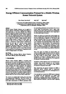
Fig. 2.5 and Fig. 2.6 show a comparison between traditional path discovery and our long-range radio assisted path discovery. The two orange nodes are sender S and receiver D. Fig. 2.5 shows the request message flooding with TTL (time to live) set to 4. The shortest path from sender to receiver is 3-hop long and in this partial topology,
" !
Figure 2.6: Long-range Radio Assisted Path Establishment
18
14 nodes broadcast the request when it reaches the receiver. Fig 2.6 illustrates the benefits of bi-directional flooding and RSSI filtering. In this example, the request is propagated from both sender and receiver and the path is established in the second round of broadcast, i.e., when node A and B broadcast their received requests. With the handshake messages including RSSI information, we assume the dotted circle and arc centered at the receiver define the region where the RSSI of the receiver’s packets is similar, i.e., RD→S . Assume the nodes on the left side of the dotted arc have RSSIs (RD ) smaller than β · RD→S . Thus they will node forward the RREQ message. Only 7 nodes broadcast the RREQ message in Fig 2.6 when the path is established.
2.3.2
Path Recovery
Path recovery is a critical component in MANETs because of the dynamic network topology caused by user mobility. We develop an efficient path recovery protocol in LAAR with the following two new techniques. Due to the page limit, we omit the detailed pseudo codes for the protocols. Partial Path Recovery: In the prior work, once a node detects a broken link, the notification will be sent back to the source by an RERR message, and then the source will launch a new path establishment process. Therefore, any single link failure will lead to a complete path establishment process which is not efficient in practice, especially if the broken link is shared by multiple active sessions. An example is shown in Fig. 2.7. In the traditional MANET routing protocols, while node V moves away causing a broken link, node U will send three RERRs to the sources which will further start three path establishment processes. In our partial path recovery solution, the node who detects the failure will notify the sources with a single RERR over the long-range radio and start path establishment processes with the destinations. Referring to the example in Fig. 2.7, node U will attempt recover the paths from U to D1 and D2. If successful, node U will notify the
19
sources about the recovered paths over the long-range radio. Meanwhile, each source node also sets a timer once receiving an RERR. If the detecting node cannot recover the path to the destinations before the timers expire, the sources will initialize the path establishment process with the destinations. Path recovery packet Data packet
S1
3 Path Establishment
1 RERR U V U
S2
S3
D1
V
V
D2
2 Path Establishment
Figure 2.7: An example of partial recovery: 3 active sessions (S1,D1), (S2,D2), and (S3,D2) share a link U→V. Node V moves away and the link U→V is broken.
Proactive Path Recovery:
The other new technique we develop is to proac-
tively start path recovery protocol before any link is broken. The basic idea is to detect weak or about-to-break links based on each phone’s mobility. Considering smartphones being the mobile nodes in our setting, we particularly use the accelerometer and RSSI measurements to determine if a node is moving away from a path it belongs to. If a node detects high movements or poor RSSIs from its neighbors, it will notify the neighboring nodes about the possible departure. Then a path recovery process will start when the node still carries out the data transfer. Once a new path is established, the neighboring nodes will update their routing tables to bypass the departing node. In practice, both accelerometer and RSSI readings are dynamic, and may not accurately reflect the user movements. We develop a heuristic algorithm that combines these two measurements to indicate if a node will cause a broken link soon. Algo-
20
Algorithm 3 Proactive Path Recovery 1: RL: avg RSSI level, SL: avg speed level, C = 0 2: When a new packet is received, update R 3: if RL is GOOD then 4: C = 0; return; 5: else if RL is POOR then 6: C = 0; Start the recovery process; 7: else 8: Measure the user’s moving speed SL C + ∆H : if SL is HIGH C + ∆M : if SL is MEDIUM 9: C= C + ∆L : if SL is LOW 10: if C ≥ τ then 11: C = 0; Start the recovery process; rithm 3 illustrates the detailed process when a packet arrives. Specifically, we define three discrete levels for RSSI values, {GOOD, FAIR, POOR}. While a GOOD RSSI indicates a stable link, a POOR RSSI will trigger a path recovery process. When a FAIR RSSI is received, our solution will start to periodically measure the accelerometer. Our intuition is that a highly mobile user with FAIR RSSIs is likely to cause a broken link. Similar to RSSI measurements, we use three levels, {HIGH, MEDIUM, LOW}, represent a user’s moving speed. Our algorithm use a variable C to track the user speed accumulation. According to the speed level, we increase C with heuristic values (line 9, ∆H > ∆M > ∆L ). When C exceeds a threshold τ , the path recovery process will be started.
2.3.3
Route Cache Management
In MANET routing protocols, every node records the known paths in a route cache to avoid the delay of path establishment. For both path establishment and path recovery protocols, route cache plays an important role. When processing an RREQ message, a node will first check its route cache and if a matching path to the destination is found, the node will reply to the source without further flooding the RREQ. However, the paths in the route cache are not verified until the node decides
21
to adopt them. In a MANET, the link conditions are dynamic and the known paths may not be stable. Using stale paths will cause path recovery once a broken link is detected and yield a worse performance than not using the route cache. In our solution, we address this issue by removing invalid paths in the cache based on the overheard packets. Two types of packets will trigger a cleansing of the route cache. First, if a node receives a broadcast RERR packet over the long-range radio indicating a broken or about-to-break link, it will search its route cache and eliminate all the paths that contain the link specified in the RERR. Second, every node will listen to the active data transmissions over WiFi or Bluetooth from the neighboring nodes even if the packets are not designated to it. By sniffing these packets (e.g., from node j to node k), node i can measure the RSSI and estimate the quality of the link j → i. If the RSSI is in the category POOR, node i will remove all the paths in its cache that contain the link j → i. Complete Protocol in Path Recovery: Here is the complete protocol. When the recovery process is initialized by node i, it first checks its path cache to see if there is another route to the destination. If an alternative route is found, node i sends a recovery message that contains the new route back to the source. When the source receives the recovery message, it will use this route for further transmission. If there is no available route to the destination in the cache, node i will send a route error message to the source, and it will start the path establishment process with the three-way hand-shake protocol with the destination. When a path is successfully established from node i to the destination, node i will re-assemble a complete path from the source to the destination. This new path will be included in a re-assemble reply message which will be sent to the source by node i over the long-range radio. Upon receiving the route error message from detected node, the source first suspends the transmission. Then, it sets a timer and waits for a re-assemble reply
22
message. If a re-assemble reply message arrives, the source will use the new path for the rest of transmissions. If the timer expires with no re-assemble reply message, the source will start a path establishment process to find a path to the destination.
2.4
System Implementation
In this section, we introduce our implementation of LAAR with off-the-shelf devices. In our prototype, we attach a TinyNode [32], which includes a long-range radio transceiver, Xemics XE1205 [19], to an Android smartphone. XE1205 operates on 915Mhz and feature low cost, low power consumption, and a communication range of 1.6 miles. We have integrated the long-range radio into assorted phones including HTC Magic phone, Nexus One phone, and Nexus 4 phone. We use PL2303 [33] USB-to-Serial bridge controller to connect TinyNode and smartphone (through either ExtUSB or MicroUSB port).
Serial Port UART
TinyNode
Smartphone Figure 2.8: Software Architecture
Software support includes programs on both smartphones and the external devices. Fig. 2.8 illustrate the design architecture with TinyNode. We have customized Android kernel and developed user space programs on smartphones to support dual radio communication. Basically, the USB port of a phone is recognized as a serial UART device (Universal Asynchronous Receiver/Transmitter) and a device file for 23
it is created under ‘/dev/’. User programs can communicate with the USB port by reading from or writing to the new device file. Communication between a TinyNode and smartphone is built on a module deployed on both sides. We have implemented data-link level protocol over this serial link (UART) communication including basic mechanisms such as checksum and retransmission. In addition, we use TUN/TAP device driver [34] to create a virtual network interface and change the routing policy on phones such that all incoming and outgoing traffic will pass through the virtual interface. In our solution, TUN is used for routing, while TAP is used for creating a network bridge. Then we have developed programs in TUN/TAP driver to process each packet. Our prototype smartphone is able to dispatch each packet to different network interfaces, either WiFi, Bluetooth, or the long-range radio. Fig. 2.9 shows two prototype smartphones equipped with TinyNode conducting a ping test with dual radio model.
Figure 2.9: Demonstration of the Dual Radio Model
2.5
Performance Evaluation
In this section, we evaluate LAAR and compare it with the conventional MANET routing protocols. The results are drawn from the experiments on basis of a small scale network and NS2 [35] simulation on basis of a large scale network. Our ma-
24
jor performance metrics are overhead, number of messages transferred, and network throughput. We compare LAAR with DSR [22], DSR-R0, and AODV-ERS [36]. DSR-R0 is the default implementation of DSR in NS2 and improves DSR with a ring-zero search scheme in the path establishment. Ring-zero search aims to reduce the overhead by firstly sending an RREQ with TTL=0. If the sender and the receiver are direct neighbors, the path would be quickly established. Otherwise, upon a timer expires, the sender will send another RREQ with a regular TTL value. AODV-ERS is an enhanced version of AODV [23] with expanding ring search, where the sender broadcasts the RREQ for multiple rounds each with an incremental TTL value. The process terminates when the destination is reached. Workloads: We consider brochure dissemination application for our evaluation. We collect a set of real brochure files for our tests considering the following cases where a MANET could help disseminate the files. (1) Advertisements in a mall: The stores in a mall may want to attract nearby customers by delivering their advertisements or coupons. (2) Subway map and schedule: Wireless signals are often poor in subway stations or tunnels. With an effective MANET, the subway administrator can simply deploy a standalone WiFi device to deliver map or schedule files to the commuters without any infrastructure support. (3) Crowded events: In an event with a large number of attendees, the infrastructure-based network may have scalability issue because of the limited capacity.
1
With a MANET setting, the attendees can easily
check the schedule of shows and other information without connecting to the Internet. Our evaluation uses the sample workload in the following Table 2.1. 1
For example, it was reported that more than 3 millions people attended the 86th Annual Macy’s Thanksgiving Day Parade and the explosive users’ demand within central park west area caused serious congestions in mobile networks.
25
Table 2.1: Brochure Dissemination Workload Case 1 2 3 4 5 6 7 8
2.5.1
Content Homedepot 20% off coupon MTA(New York) Map Target Black Friday 2014 MBTA(Boston) Schedule AT&T Cyber Monday Sale 2014 NYC Thanksgiving Parade Nordstrom Anniversary Sale 2014 Mall of America Direction
Format PDF PNG HTML PDF PDF PDF PDF SWF
Size 213KB 344KB 915KB 1.2MB 2.1MB 2.8MB 4.2MB 5.2MB
Experimental Results
First, we build a small scale Ad-Hoc network consisting of 6 Android smartphones equipped with the long-range radio. The phone-to-phone Ad-Hoc mode is supported with WiFi and WiFi-Direct. In our experiments, the smartphones are placed at the fixed positions, i.e., the mobility is not considered. We mainly evaluate the data throughput and the performance of the path establishment protocol. The hop distance between the source and destination ranges from 1 to 5. Fig. 2.10 plots the experimental results with the workload in Table 2.1. The bars show the time consumption of the transmission in each case versus the length of the path. Apparently, the overhead grows along with file size and path length. For example, disseminating 2.1MB (case 5) and 4.2MB (case 7) files takes 4.178s and 6.424s respectively for a 2-hop path. The overheads are increased to 25.575s and 30.134s for a 3-hop path. We observe that a MANET is effective for delivering up to a few Megabytes of data to nearby nodes. For a large file over a long path, e.g., case 8 (5.2MB) with a 5-hop path, the overhead may not be acceptable for users. In practice, considering the dense user population and possible user content sharing, we expect a short path length for any communication session. In addition to the overall performance, we also evaluate the breakdown overhead and try to answer the following questions.
26
Complete Time (second)
Complete Time (second)
2-Hop Route
35 30 25 20 15 10 5 0
3-Hop Route
35 30 25 20 15 10 5 0
1
2
3
4 5 6 Case Number
7
8
1
2
3
70 60 50 40 30 20 10 0 1
2
3
4 5 6 Case Number
7
8
5-Hop Route Complete Time (second)
Complete Time (second)
4-Hop Route
4 5 6 Case Number
7
8
70 60 50 40 30 20 10 0 1
2
3
4 5 6 Case Number
7
8
Figure 2.10: The experimental performance of overhead with different path lengths
Can we use the long-range radio for data delivery? The protocol design could be much simplified if the long-range radio can carry out the data transmission. We have conducted the same experiments with direct transmission between two TinyNode devices. The results are shown in Fig. 2.11a. Compared to Fig. 2.10 , the time consumption with the long-range direct link is much higher. Fig. 2.11b further compares the throughput of direct long-range radio link with hop-by-hop transmission along a 5-hop path. In this experiment, we use “iperf” tool to record the throughput every 20 seconds. We observe that hop-by-hop delivery yields a much higher throughput (with a high variance) even over a long path. Overall, we conclude the long-range radio works well for small management packets, but is not suitable for bulk data transmission.
27
Throughput (Kbps)
Complete Time (second)
700
250 200 150 100 50
600 500
TinyNode 5-Hop Route
400 300 200
0 1
2
3
4 5 6 Case Number
7
100
8
20
(a) Direct link
40
60 Time
80
100
(b) Direct link v.s. 5-hop path
Figure 2.11: TinyNode data delivery performance
2.5.2
Simulation Results
In addition to experiments, we conduct simulation with NS2 to evaluate LAAR in a large scale network.
2.5.2.1
Simulation Settings
In the simulation, we consider the brochure dissemination application in a mall. We run the simulation in following two settings. • Single store: In this setting, there is only one store trying to send out brochures to the nearby shoppers. We assume that the store periodically broadcasts a short message including a link to the brochure file over the long-range radio. The users can use the link to fetch the brochure. We assume that N users receive the short message and α ∈ [0, 1] portion of them will be interested in it, i.e., α × N users will download the brochure. • Multiple stores: In this setting, there are multiple senders in the mall. Similar to the previous setting, the senders first use periodical short messages over the long-range radio to notify the users.
28
The parameters in NS2 are set as follows. First, we adopt two-ray ground reflection model and constant speed propagation delay model for wireless signal prorogation. In addition, each node in our LAAR protocol is set with two radios. We modify the NS2 to support two wireless interfaces. The frequency of the long-range radio is set to be 915MHz, and the communication range is configured to be 2500m in receiving (RX) and 3000m in carrier sensing (CS). The other regular radio (short range) is configured to work at 2.4GHz, and the RX and CS ranges are set to be 50m and 100m respectively. For the results shown in this chapter, β is set to 0.9 for the RSSI-guided flooding. The users in the simulations follow a manhattan grid mobility model [37] with a maximum moving speed of 2m/s. At an intersection, the probability of going straight is 0.5 and taking a left or right is 0.25 each. We generate mobility traces with different numbers of users, and in each trace, users randomly select the initial positions inside a store or on a corridor. For all the tested protocols, we set RREQ’s default TTL to 5 if applicable. For speed level with user mobility, the three discrete values in Algorithm 3 are defined LOW ( 1.5m/s ). In addition, ∆H = 2, ∆M = 1, δL = 0, and τ = 3. 2.5.2.2
Single Store
In this setting, we choose Nordstrom (case 7) as our sender and conduct the simulations with different values of the parameters N and α. For each particular setting, we randomly generate 100 mobility traces for tests, and present the average values in the following figures. Path establishment: First, we set N to 200 and 300, and change the value of α to control the total concurrent sessions in the network. The overhead performance of initial path establishment is shown in Fig. 2.12.
29
In our setting, the average number of neighbors is 23.9 and 34.3 for N = 200 and N = 300 respectively. The dense topology can lead to a serious congestion in the existing routing protocols, for example, as shown in Fig. 2.12b, to construct 9 (3% × 300) concurrent sessions, DSR, DSR-R0 and AODV-ERS uses 514ms, 598ms and 459ms, respectively. However, in LAAR, the overhead of path establishment remains low, because our design reduces the number of messages transferred mitigating the
800 700 600 500 400 300 200 100 0 1%
Time Cost(ms)
Time Cost(ms)
effect of congestion.
LAAR DSR DSR R0 AODV-ERS
2%
3% α
4%
5%
800 700 600 500 400 300 200 100 0 1%
LAAR DSR DSR R0 AODV-ERS
2%
(a) N = 200
3% α
4%
5%
(b) N = 300
700
LAAR
600
DSR
500
AOVD-ERS
Messages Transferred
Messages Transferred
Figure 2.12: Average overhead of path establishment (single store)
DSR-R0
400 300 200 100 0
700
LAAR
600
DSR-R0
500
AOVD-ERS
DSR
400 300 200 100 0
1%
2%
3% α
4%
5%
1%
(a) N = 200
2%
3% α
4%
5%
(b) N = 300
Figure 2.13: Average number of messages transferred to establish path in single store: varying α with 200, 300 users
30
Fig. 2.13 illustrates the number of messages (RREQs) transferred in the entire network. The bars indicate a similar trend in all the protocols. Our solution LAAR significantly outperforms the other three protocols. Overall throughput:
We use throughput as an overall performance metric
taking full mobility trace and link breaks into consideration. Since DSR and DSR-R0 use the same path recovery protocol, we do not include DSR-R0 in this test. Instead, to better study the impact of stale routes in the cache, we evaluate a DSR protocol that does not use route cache. The results are compared in Fig. 2.14. LAAR maintains a high throughput with different α. For example, with N = 300 and α = 3%, the throughputs of DSR, DSRNC, AODV-ERS and LAAR are, 34.1, 30.7, 50.8, 289.1Kbps. LAAR’s throughput is more than five times the throughput of the second best protocol, AODV-ERS. The major reason of the significant improvement is the efficient path recovery protocol in LAAR. Our solution greatly reduces the overhead and congestion during a recovery process, and also improves stability of the selected path and the effectiveness of the
400 350 300 250 200 150 100 50 0 1%
Throughput(Kbps)
Throughput(Kbps)
route cache.
LAAR DSR DSR-NC AODV-ERS
2%
3% α
4%
5%
(a) N = 200
400 350 300 250 200 150 100 50 0 1%
LAAR DSR DSR-NC AODV-ERS
2%
3% α
(b) N = 300
Figure 2.14: Average throughput in single store
31
4%
5%
2.5.2.3
Multiple Stores
Finally, we test with three stores, Target (case 3), AT&T (case 5) and Nordstrom (case 7) as our senders. Each store tries to disseminate its brochure listed on Table 2.1. In our configuration, the α for each store’s brochure is the same. Thus, the total number of transmissions in the network is 3 × α × N . We collect the throughput from
350
350
300
300
Throughput(Kbps)
Throughput(Kbps)
each transmission session and show the average result for each different α value.
250 200
LAAR
150
DSR-NC
DSR AODV-ERS
100 50 0 1%
2%
3% α
4%
5%
250 200
LAAR DSR
150
DSR-NC
100
AODV-ERS
50 0 1%
(a) N = 400
2%
3% α
4%
5%
(b) N = 500
Figure 2.15: Average throughput in multiple stores (3 stores)
Overall throughput: Fig. 2.15 plots the throughput with different values of α when N = 400, 500. Obviously, LAAR performs the best among the four tested protocols. For example, in Fig. 2.15a, the throughputs of LAAR, DSR, DSR-NC, AODV-ERS are 327.4, 67.0, 32.5, 54.4Kbps with α = 3%, respectively. We also find that the throughput of LAAR is not always inversely proportional to the increase of α. For instance, in Fig. 2.15b, the throughputs are 306.1, 334.4Kbps for α = 1%, 2%. With more users involved in the transmission, our techniques of proactive path recovery and route cache management wii be more effective helping improve the throughput performance. Fig. 2.16 shows the throughput with different number of users (N ). The values of α in Fig. 2.16a and Fig. 2.16b are set to 5% and 15%, respectively. Again, LAAR outperforms the other three protocols.
32
300
300
250
250
Throughput(Kbps)
Throughput(Kbps)
LAAR
200 LAAR
150
DSR DSR-NC
100
AODV-ERS
50 0 400
500
600 N
700
200
(a) α = 5%
AODV-ERS
150 100 50 0 400
800
DSR DSR-NC
500
600 N
700
800
(b) α = 15%
Figure 2.16: Average throughput in multiple stores (3 stores)
2.6
Summary
This chapter presents LAAR, a new dual radio model for smartphone-based AdHoc networks. We integrate a long-range radio to help improve the performance of path establishment and recovery which are critical components in the routing protocols. The experimental and simulation results show that LAAR dramatically improves the performance.
33
CHAPTER 3 PASSIVE DELIVERY IN AD-HOC NETWORKS
In Chapter 3, we focus on short message dissemination in the proximity. It represents a category of applications with high potential if communication between nearby devices are well supported. For example, a user may want to share his recent tweets or facebook messages with other people sitting in the same room; a police car on site of car crash may disseminate the accident information to other cars within one mile distance; a student in library may chat with his friend in another classroom via instant messenger; a bunch of sport fans may want to share the comments with each other on the same game they enjoyed; a victim of crime or natural disasters may want to ask for help when there is no cellular network or not cannot use it. The current location-based service architecture is still based on a centralized client-server model, where a user submits his location to a server and obtains the customized data he needs. This conventional model quite limits the application scope and may hinder wide deployment of location related mobile applications because of the following disadvantages. First, it requires Internet connection even when a sender and receiver are adjacently located, which will unnecessarily increase the Internet traffic burden and users’ bandwidth cost. With this requirement, in addition, applications are not robust against catastrophic infrastructure failures. Furthermore, a data consumer has to have prior knowledge of the data providers, e.g., the URL of the server. There is no general channel for users to browse all available service resources nearby without registering for each and every one of them.
34
Node with Data Scanning Node
Scan range
Message Delivery
Figure 3.1: Passive Broadcast Model
We argue that Ad-Hoc network model is a complementary alternative that can effectively help solve all the above issues. In practice, however, creating and maintaining a direct link between two nearby devices which is the building block of an ad-hoc network is costly. For example, both Bluetooth and WiFi-Direct require a slow initial phase of discovering nearby peers and handshaking to establish a connection. It is especially inefficient for transferring a small amount of data. In addition, connected link may bring with it a security risk because one device might be able to access all exposed services on the connected device (e.g., in Bluetooth). In this chapter, we build a local data dissemination system upon a new communication model, called passive broadcast. It is a connectionless and receiver-initilized model where each node periodically scans other nodes in the communication range and obtains their data if available (see Fig. 3.1, i.e., each scan is a many-to-one communication. The representative carriers of passive broadcast in reality include Bluetooth and WiFi-Direct, both of which define a mandatary ‘peer discovery’ function to fetch basic information about nearby devices. This function can be easily extended to implement passive broadcast mechanism without modifying the existing network protocol stack. In passive broadcast, the cost for establishing and maintaining direct links is negligible and our experiments show that the communication range is expanded compare to the established connection over the same radio interface. In addition, the feature
35
of fetching messages from multiple nearby devices is desirable for applications that spread messages in the proximity.
3.1
Related Work
This work is related to prior research on mobile social networks, overlay P2P dissemination, and delay tolerant networks. Information dissemination has become more and more important in mobile social networks, such as [38–40], which aim at data dissemination in resource-constrained opportunistic networks, broadcasting from superusers and ferrying messages in intermittently connected mobile networks. Point&Connect [41] implements pointing gestures of moving one device towards another in order to enable spontaneous device pairing. Musubi [42] provides a decentralized trusted social services on personal mobile devices. And BubbleRap [43] utilizes group membership information to improve standard unicast routing. In [44], the authors propose a gossiping-based approach, where each node forwards a message with some probability, to reduce the overhead of the routing protocols. 7DS [45] is developed to address network disruption problem in mobile networks by providing storecarry-forward communication. However, it only concerns data as store-carry-forward manner for disruption-tolerant applications which is very limited. [46] proposes to use data diffusion to reduce the query delay in DTNs. They use theoretical models to analyze the data diffusion process and compare the performance of the their proposed diffusion schemes in terms of diffusion speed and query delay. In addition, there is other prior work that helps better understand characteristic of DTNs such as [47–50]. For example, [47] is the rst to study multicast in DTNs from the social network perspective. They study multicast in DTNs with single and multiple data items, investigate the essential difference between multicast and unicast in DTNs, and formulate relay selections for multicast [48] studies human contact-based traces and designs SNAMD scheme that makes use of such information to efficiently deliver
36
multicast messages. The authors in [49] compared the asymptotic performance of Interest-Based forwarding and from both the theoretical and experimental point of view. And SimBet [50] first introduces social network analysis in the context of delay tolerant networks. It uses ego-centric centrality and its social similarity. However, the focus of our problem is based on a different communication model and our objective is different. Passive broadcast is a receiver-initialized connectionless communication based on many-to-one delivery in each scan. Moreover, we target on a distributed and collaborative solution that efficiently disseminate messages in proximity. One project closely related to our passive broadcast model is called Dythr [51] which lets a phone broadcast a WiFi hotspot with the SSID being the message. This method actually is from the opposite direction of ‘active’ delivery as every node frequently injects messages into the wireless channel. In [52], Huang et al. proposed PhoneNet. This method uses a central server to establish links between devices connected to a WiFi network and then allows devices connected on local networks to connect directly. In [53], the authors use Bluetooth service discovery protocol to find common interests between two users. Similar to our proposed work, no connection is established and each user stores the keyword about his interest in Bluetooth service ID. However, this work is for two-user communication while our problem is set in a multiple user environment and our goal is to determine each device’s schedules to achieve the efficiency.
3.2
System Model
Our target problem in this chapter is to enable nearby smartphone users to share information. In this section, we introduce basic components and sketch of our solution.
37
3.2.1
Communication Model
Our solution is based on the new passive broadcast communication model, where each sender buffers its broadcast data locally and the receiver initializes the transmission and fetches all available data from nearby nodes. In this model, when having a message to deliver, a node puts it in a buffer, but does not know when the message will be sent. On the other hand, each node periodically scans other nodes in the communication range and obtain the data in their buffers if available, i.e., each scan is a many-to-one communication. We have implemented this model based on the mandatary ‘peer discovery’ function in both Bluetooth and WiFi-Direct. In the rest of this chapter, we take Bluetooth as a platform instance to introduce our solution. Basically, we use the field of ‘device name’ to carry target payload data. When a user intents to send a message, he assigns the message to his phone’s Bluetooth device name. When other phones conduct peer discovery, the message will be sent over. The length of device names is usually limited, e.g., a Bluetooth’s device name in Android can be up to 248 bytes. A large message can be fragmented to fit in and a phone can periodically change the device name to rotate multiple messages or fragments.
3.2.2
Smartphone Operations and States
Assume there are n smartphone nodes ({p1 , p2 , . . . , pn }) and this chapter considers a network model where all the phones are within each other’s Bluetooth communication range. There are two basic operations for each smartphone pi , scan and update message. The first operation is the regular peer discovery process while the second one is to change its own device name to a new message. Update message operation can be finished instantly. But scan process has a long overhead. For Bluetooth, according to the standard and our experiments, a scan operation usually takes 10 ∼ 12 seconds to finish. Therefore, we further define two states for each phone: when a
38
phone is conducting scan (peer discovery), it is in scanning phase; otherwise, it is in idle phase. For each message, we define its active period as the duration when the message is available for scanning, i.e., after the message is put on the device name and before it is replaced by the next message. If a phone finishes a complete scan during a message’s active period, the message will be surely scanned by the phone. If the active period starts or ends during a scanning process, the phone has a certain probability to receive the message. We will present detailed analysis later in Section 3.4. We assume that the scan schedule has been pre-configured by each phone based on its own performance concerns, e.g., power consumption and urgency of getting new messages. We use Ti to represent pi ’s scan interval which is defined as the interval between the end of the prior scan and the beginning of the next scan, i.e., the length of pi ’s idle phase. Additionally, we use Ui to indicate the message update interval of pi , i.e., pi changes its device name once every Ui time units. Different from Ti , Ui ’s value can be dynamically changed as it does not incur any extra computation overhead or power consumption. Furthermore, we define S as the length of scanning phase, which is a constant for all phones. In our solution, each phone and each active message has a unique identifier defined as follows: • Phone ID: In this chapter, we use the MAC address as each phone’s identity. When scanning nearby devices, a phone automatically obtains their MAC addresses and is able to recognize these phones later. • Message ID: Each message can be identified by its owner’s MAC address and a local index number. For example, aa:bb:cc:dd:ee:ff.12 represents a message from the phone with a MAC address of aa:bb:cc:dd:ee:ff and its index number on that phone is 12. In our solution, each index number is incremental with new messages and set up to 255 after which it will be reset to 0. 39
3.2.3
Message Format
In our solution, the device name is divided into two segments, header and payload. Similar to other network protocol, ‘header’ field contains control and management data and ‘payload’ stores the messages being broadcast. The header includes the following fields: • Scan interval T : Each phone pi uses one byte to represent its own scan interval Ti in the unit of second. • Index range of active messages: Each phone uses two bytes to specify the index number range of its active messages. We assume each user apply the policy that only the most recent messages are considered for dissemination, e.g., the most recent 10 messages, and the messages generated in the past 5 hours. • Message reception feedback: Each phone includes a message reception feedback to indicate the current state of the reception. Our solution uses a simple bitmap to represent this feedback information. Namely, every message is flagged by one bit in the feedback, ‘1’ indicates ‘received’ and ‘0’ means ‘absent’. We assume that a function f can convert a MAC address to a numeric value, thus all phones can be ordered according to their MAC addresses. In the bitmap feedback, the messages from different phones are ordered by their owners’ MAC addresses. The following Table 3.1 lists some notations we use in the rest of the chapter. n/pi Ti /Ui S ti f ki M
number of smartphones/the i-th phone scan interval / update interval of pi execution time of one scan execution time for pi to receive all messages a function that converts a MAC address to a numerical value number of messages generated by pi set of all message IDs in the network Table 3.1: Notations
40
3.3
Message Dissemination with Passive Broadcast
In this section, we present our solution PASA that disseminates local messages based on passive broadcast model. We further provide numerical analysis to derive the optimal parameters for our solution.
3.3.1
Problem Formulation
Recall that we consider all the phones {p1 , p2 , . . . , pn } are within each other’s communication range. Each phone pi holds ki messages to propagate to other phones. Assume each smartphone is aware of other phones’ scan intervals after an initial scan. Without loss of generality, we sort all smartphones in the ascending order of their scan intervals, i.e., ∀i, j ∈ [1, n], if i < j, then Ti < Tj . Let ti represent the time phone pi spends in receiving all the messages. Our objective in this chapter is to P minimize i ti . The essential goal of our algorithm is to determine the update interval for each phone so that all phones can collaborate to disseminate all messages quickly. Out solution is based on an important property defined in the following Theorem 1. Theorem 1. If a phone set its update interval to be Tn + 2 · S, its message can surely be scanned by all other phones. Proof. For any phone pi (Ti ≤ Tn ), apparently there must be a complete scan during a period of Tn +2·S. Thus, the message will certainly be scanned by every phone. 3.3.2
Design of PASA
We present a solution with two stages. In the first stage, every phone simply sets Ui to be a constant α and rotates its own ki messages. In the second stage, each phone set Ui = Tn + 2 · S and iteratively update the device name by one of the messages generated by its own or received from the first stage. The strategy of updating messages, however, varies depending on each phone’s status during the
41
second stage. We classify all phones into two categories and each category executes a different algorithm. The first category is called complete phones which includes P all the smartphones that have received all i∈[1,n] ki messages. The other category, incomplete phones, is the complement of the first stage and includes the phones that have not received all messages. As the update interval is fixed as Tn + 2 · S, our design focus is message updating algorithm in the second stage. In the rest of this section, we develop two algorithms, one for incomplete phones and the other for complete phones. Our basic intuition is to let all the smartphones assign the most wanted messages to the device names so that they can help other phones to speed up their second stages. In addition, we intent to avoid duplicate messages in the second stage. It is apparently inefficient if multiple phones put the same message on their devices’ names. In the stretch of our solution, we give incomplete phones higher priority to select messages as the messages that incomplete phones can contribute in the second stage are limited. Complete phones, on the other hand, will estimate incomplete phones’ choices and select other desired messages to serve in the second stage. We use M to represent the set of all message IDs in a given network, i.e., in our P setting, M includes i ki items. Assume all message IDs in M are sorted according to a pre-defined numerical conversion and let mi represent the i-th item in M . Each phone is aware of M after the initial scan. In addition, each phone maintains a two dimensional matrix M R to indicate the message reception status in the network, where M Rij = 1 if phone pi has received message mi (otherwise M Rij = 0). For each phone, this matrix M R is built upon the feedbacks from other phones. With the assistance of M R, each phone can derive sufficient information for the next stage. First, each phone can identify all the complete phones and incomplete phones, i.e., P pi is a complete phone if j M Rij = |M |. Let IP and CP respectively represent the set of incomplete phones and complete phones each phone constructs. Second,
42
each phone knows which messages it has received are needed by other phones. We let each phone pi build a set of candidate messages, indicated by Ci , including all the messages that are useful for some other phones and could be put on the device name in the next stage. By definition, each message mj ∈ Ci must satisfy M Rij = 1 and P h M Rhj < n. In addition, we assume each phone has a different priority value based on the phone ID. Our algorithm will use this priority value to avoid unnecessary duplicate message selections from multiple phones. If a message is chosen by multiple phones, only the one with the highest priority will put it on the device name and the others have to yield and select other messages. Specifically, we assume a pre-defined the function f could convert a phone ID to a numerical value for comparison, i.e., pi has a higher priority than pj if f (pi ) > f (pj ). Message update for incomplete phones: In our solution, an incomplete phone applies the following Algorithm 4 in the second stage. Algorithm 4 Choose the Message for Incomplete Phones 1: Identify all incomplete phones (construct IP ) 2: Sort the set IP in the descending order of each phone’s priority 3: for each incomplete phone pi do 4: Construct its candidate set Ci 5: Sort Ci in the ascending order of the number ofPphones having received the messages, i.e., for each message mj , the value of h M Rhj . 6: for i = 1 to |IP | do 7: Let pj be the i-th phone in IP , choose the first message of Cj : msgj = Cj [1] 8: for each incomplete phone ph ∈ IP do 9: Remove Cj [1] from Ch
In Algorithm 4, each incomplete phone first identifies all incomplete phones (the set IP ) and sorts them based on their priority values. Additionally, each phone forms the candidate sets of all incomplete phones using the information from M R (Lines 3–6). The candidate messages are also sorted by the number of phones that have received them (Line 5). In our algorithm, therefore, the first message in each
43
candidate set is the most wanted messages. The main message selection process is in Lines 7–12. We use msgi to record the choice of pi . The loop starts from the phone with the highest priority to the one with the lowest priority. Within the loop, each phone picks the first message in the candidate set for updating message in the second stage. Upon a message msgj is selected, all candidate message sets are updated by removing msgj to avoid redundant message selections. Eventually, for a phone pi , msgi will be the message to be put on the device name. The time complexity of Algorithm 4 is bounded by O(n2 ). Message update for complete phones: The algorithm for a complete phone to update message is similar to Algorithm 4. Due to the page limit, we omit the pseudo-codes here. Each phone needs to construct the set of all complete phones CP and derive the candidate message set for each of them. An extra step for a complete phone is that it has to execute Algorithm 4 before making its own choice. All the messages that have been selected by incomplete phones will be eliminated from complete phones’ candidate sets. The remaining messages in the candidate set are also sorted according to the number of phones that need them. The same as in Algorithm 4, each phone selects the header message in the sorted list of candidate messages.
3.3.3
Parameter Optimization
In this subsection, we analyze the performance of the solution presented above and derive the optimal value of α. Essentially, we aim to express the objective as a function on α. Our analysis is based on a general function P(x, y) defined to represent the probability that a phone with scan interval of x can receive a message from another phone with update interval of y. In another word, P(Ti , Uj ) is the reception probability for pi to receive a message from pj . We will present how to calculate P(x, y) in Section 3.4.
44
We use the following Theorem to estimate the execution time for each phone to receive all messages, i.e., the value of ti . Theorem 2. The execution time for phone pi to receive all messages is expected to be ti = kmax · α + r · (Tn + 2 · S), P (kmax−ki )·α where kmax is larges value of ki , and let c1 = , c2 = (1 − ki OP T then 10: OP T = c, i∗ = i 11: A = A + ui∗ , CUi∗ = CUi∗ + 1, CM = CM + 1 12: if CUi∗ = τ then 13: users = users - ui∗ Algorithm 6 describes the details of the initial assignment stage. Firstly, the owner, uo , initializes the selected user set, A and counter of replicas, CM . In addition, it needs to combine its accessible neighbors into a set named users. This set excludes the users that have already reached their maximum number of messages threshold (line 1). When the set users is non-empty and CM is still under the threshold, for every ui ∈ users, it computes the activation period if ui is chosen to be a message holder by using the message’s activation function in a LLM C . The algorithm continues until it finds the largest c among all the ui ∈ users (lines 2–10). After choosing the 70
candidate ui from ANu0 , we update selected user set and the counter of replicas for this message. Moreover, we add u∗i to the selected user set and refresh the number of hosted messages of uo . Finally, it keeps monitoring whether ui has meet its limit. If it is, we remove it from the candidate user set. (lines 11–13). Algorithm 7 Message Delegation (by the selected uo ) 1: users = {ui | CUi < τ and ui ∈ ANo }, A = {}, CM = 0 2: holdersmj = {un | mj ∈ HUn }, OP T 3: while holdersmj 6= φ and excludes uo do 4: for Every un ∈ holdermj do 5: n = n∗ 6: for t = 1 to LLM C do 7: if yi (t) = 1 then 8: Fj (t) = 1 9: holdersmj = holdersmj − un∗ 10: while users 6= φ and CM < θ + 1 do 11: for Every ui in users do 12: for t = 1 to LLM C do 13: if yi (t) = 1 then 14: Fj (t) = 1 P C 15: OP T ∗ = LM Fj (t) 1 16: if OP T ∗ > OP T then 17: OP T = OP T ∗ , DU = ui
Without the coordinator’s assistance, the owner may fail to choose the best users to host the message due to the limit of accessible neighbors. In this case, after the initial assignment, the selected users keep tracking to see if there is any better user that can hold the message and lengthen the total active time. Algorithm 7 illustrates how uo delegate the message mj to a better user. First, it initializes the users set, the selected user set and message mj ’s current holder set which is the set A from algorithm 6 (lines 1–2). Then, we calculate the activation function , Fj (t), without uo ’s hosting (lines 3–10). Next, the algorithm computes whether the active time becomes longer if one of the users in uo ’s available neighbors is chosen to host mj . After enumerating all the available neighbors, we select the user that can return the maximum OP T (lines 11–13).
71
4.4
Implementation And Evaluation
In this section, we will first introduce the system implementation of our MMB system and then present the performance evaluation results from our experiments and simulation.
4.4.1
System Implementation
In the implementation, we take advantage of the MMB system in the application of warning the Rogue Access Point (RAP) in an airport when users are not able to or very costly to connect to the Internet. In this scenario, users report the RAP by changing their Bluetooth name and publish the information to the MMB. When a user finds a possible RAP, it changes its Bluetooth name to “MMB:Mac:X”, where MMB is a prefix that is used to filter out unrelated Bluetooth devices, Mac is the RAP’s MAC address and X stands for 1 or 2 which indicates rogue access point or slow speed access point. We implement the prototype as an Android application for smartphone. However, for off-the-shelf phones, as long as they have Bluetooth modules and can change their namespaces, they can contribute to the system by reporting the suspected access points. Fig. 4.2 is a set of screen shots of the Android application. Upon opening the application, the users need to initiate scanning to discover the nearby MMB warning messages (the left figure of Fig. 4.2). Then, they can start discovering the active nearby Wi-Fi hotspots and the reported access points are clearly marked (the middle figure of Fig. 4.2). When a user attempts to click “connect” button, the warning message will pop up (the right figure of Fig. 4.2).
4.4.2
Environment Settings
In this subsection, we discuss the details of the environment settings in both experiments and simulations.
72
Figure 4.2: Rogue Access Point warning application of MMB system
4.4.2.1
Experiments
In the experiments, we use 6 Android smartphones that include LG Nexus 4, Nexus 5, Google Nexus 7 and Samsung Galaxy S4. During the experiment, we distribute the smartphones on the desks in our lab which is around 20m2 to form a fully connected network. The state schedule, Ti and Ii , is preloaded in each phone. In addition, other user settings, like messages and thresholds, are pre-configured.
4.4.2.2
Simulations
We use the Crawdad dataset from Dartmouth [60] for the simulation. The particular dataset we use is Sigcomm 2009 trace that contains Bluetooth encounters, opportunistic messaging, and social profiles of 76 users of MobiClique [61] application. Based on the length of encounter time and activity, we filter out the users who only appear in a short period and lack of activities. Then, there are 52 users left whom we consider as the valid clients. We drive the encounter length and number of social messages from the dataset as the parameters. In the simulation, we randomly pick up the users from the valid clients pool. Due to lack of the Bluetooth OFF state data, we assign each user a OFF length randomly so that each user has a state
73
schedule. Finally, the parameters are fed to our simulator to examine the Mobile Message Board system.
4.4.3
Performance Evaluation
In this subsection, we present the evaluation results from both Android smartphones experiments (small scale) and simulation (large scale). We consider the following four different cases for our evaluation. • Case 1: Only one message generated by one user in the MMB system. • Case 2: Multiple messages generated by the same user. • Case 3: One message generated by multiple users. • Case 4: Multiple messages generated by different users. The major performance metric we exam is the Activation Rate (AR) for each message. For each mj ∈ M , its activation rate is defined as, P ARj =
t∈[0,LLM C ] cj (t)
LLM C
(4.6)
where, according to Table 4.1, c(t) is the indicator of whether mj is active at time t and LLM C is the function that returns the least multiple common of all the users’ state schedules in the MMB system.
4.4.3.1
Experimental Results
We manually set the required state schedule and randomly choose the limit number of messages per user in the range from 1 to 3 for each phone as shown in Table 4.2. In the experiments, we mainly focus on the parameters’, τ and θ, impact on activation rate. (the parameters’ definitions are in Table 4.1). As for the message owners, we randomly pick from the six candidates for different cases. 74
uid 1 3 5
T I τ 10 10 3 15 25 1 15 20 2
uid 2 4 6
T I τ 15 10 1 10 20 1 10 15 2
Table 4.2: Parameters
Fig. 4.3 plots the average activation rate per message under different θ. As the figure displays, if the θ = 1, it suggests each message only has one host. Except case 3, the activation rate of the other three cases is very low (less than 0.6). The reason lies in the fact that for the case 1, 2, and 4, each message can only has one host controlled by θ. However, in case 3, since different users generate the same message, it can bypass the limit of θ. The activation rate grows along with the replicas increasing since the more hosting users get involved, the less OFF state is in each period.
1
0.75
Activation Rate
Activation Rate
1
Case 1 Case 2 Case 3 Case 4
0.5 1
2 3 4 Number of replicas
0.75 Random t Maximum t
0.5 5
1
Figure 4.3: Activation Rate versus number of replicas (θ)
2 3 4 Number of replicas
5
Figure 4.4: Comparison of random and maximum τ values (case 4)
Then we focus on the impact of τ which controls the maximum number of messages each user can host. As shown in Table 4.2, τ is randomly selected from 1 to 3. Fig. 4.4 compares the case 4 under the random setting above and the maximum setting that assigns every user the limit of 3 messages. The figure indicates that the maximum τ setting can improve the activation rate. The difference of state schedules results in
75
the improvement since the user with largest ON state portion, user 2, can hold more messages (1 v.s 3 ). 4.4.3.2
Simulation Results
In the simulation, we use the parameters that derived from the trace. However, it lacks the records of Bluetooth OFF state and messages replicas. Therefore, we
1
Msgs-20 Msgs-30
Activation Rate
Activation Rate
randomly pick the OFF state from 5 to 50 and the number of replicas from 1 to 5.
0.75
1
Msgs-20 Msgs-30
0.75
0.5
0.5 10
1
20 30 40 50 Number of Users
Figure 4.5: Activation Rate (case 4) with random number of replicas
2 3 4 5 Number of Replicas
Figure 4.6: Activation Rate (case 4) with fixed number of replicas and 30 users
Fig. 4.5 illustrates activation rates (with coordinator) under different number of users. In addition, the number of messages is set to 20, 30. Consequently, the activation rate grows with the user size increase. The more users are in the system, the more choices are for each message. The figure also implies a fact that the activation rate is higher for 20 messages than 30. It can be attributed that, with fixed user size, less messages in the system results in more choices for each message. Fig. 4.6 plots the activation rate (with coordinator) under different fixed replicas (all messages has the same θ) with 30 users. Since the user size is fixed, the activation rate goes up along with the replicas. Moreover, the Msg-20 experiment has a higher activation rate than Msg-30. It reflects the fact that with the same user group, the smaller message set size results in more choices for each message. 76
Activation Rate
with-coordinator w/-coordinator
1
0.75
0.5 10 20 30 40 50 Number of Users (Msg-30) Figure 4.7: Activation Rate (case 4) with fixed number of replicas and 30 messages
Next, we compare the two approaches, with and without the coordinator. To compensate the absent of coordinator, in the second approach, the message, after initial assignment, will be delegated to other users if it can improve the activation period. It takes some time for the delegation process. Therefore, the simulation is configured to keep running for two periods (two LLCM ). Fig. 4.7 compares the two approaches with Msg-30 under different size of users. As shown on the figure, two approaches achieve the same performance with 10 users. This is because the central message assignment by the coordinator and initial message assignment by the owners choose the same holders for the messages. Without the coordinator’s assistance, the second approach fails to choose the optimal users for some messages in the other settings that results in the decrease of average activation rate in the system. However, message delegation can compensate some of the decrease. For example, in user 20 setting, the average activation rate is 0.77 after message initial assignment. The overall activation rate improves to 0.82 in two periods after the delegation.
77
4.5
Summary
This chapter presents a Mobile Message Board (MMB) system for smartphone users to share messages in a target area. Our solution is built on ad-hoc communication model without the support from the Internet. We present algorithms that appropriately manage the messages on each participating phone to maximize the message availability in the system. In addition, we have implemented our solution on off-the-shelf phones. Our evaluation based on experiments and simulation shows that our system is efficient and effective for disseminating messages in the proximity.
78
CHAPTER 5 SKYFILES: EFFICIENT AND SECURE CLOUD-ASSISTED FILE MANAGEMENT
In this chapter, we develop Skyfiles which is a system for smartphone users to manage their files in the cloud storage. Our basic idea is to launch a cloud instance to assist users to accomplish the file operations. It is motivated by the fact that the cloud instance is inexpesive and sometimes free. For example, Amazon Web Service (AWS) [62] provides 750 free Micro instance hours per month. By using the resources of the instance, smartphone users will significantly reduce the bandwidth consumption for file operations. Skyfile still does not require users to keep local copies of files, but provides advanced and secure operations.
5.1
Related Work
In the past few years, cloud computing and storage technology gain more and more attention in mobile applications. In [63], a survey studies offloading computation to the cloud side with the objective of extending smartphone battery life. MAUI [64], Cuckoo [65] and ThinkAir [66] implement an Android framework on top of the existing runtime system. These three systems are easy to deploy because they only need to access to the program source codes, and they do not require modifying the existing operating system. They provide a dynamic runtime system, which can, at runtime, decide whether a part of an application is better to be executed locally or remotely. Besides offloading computation for the mobile devices, SmartDiet [67] aims at offloading communication-related tasks to cloud in order to save energy of smartphones. 79
In addition to offloading services, another major utilization of cloud computing for mobile users is to enrich the storage size on smartphones. CloudCmp [68] studies on a comparison about user achieved performance among different storage providers by running benchmarks. In [69], the authors focus on the impact of virtualization on Dropbox-like cloud storage systems. Focusing on Amazon Web Service, a cloud storage infrastructure provider, [70] shows that the perceived performance at the client is primarily dependent on the client’s network capabilities and the network performance between client and AWS data center. Furthermore, the authors of [71] investigate Dropbox users to understand characteristics of personal cloud storage services on mobile device. Their results show possible performance bottlenecks caused by both the current system architecture and the storage protocol. While cross-platform cloud storage services provide great usability, the increasing amount of personal or confidential data entrusted to these services poses a growing risk to privacy [72–75]. There are some prior works attempting to use cloud computing to enhance security and privacy of mobile devices. Authors in [76] provide a survey to explore the security and privacy issues in cloud computing. CloudShield [77] presents an efficient anti-malware smartphone patching with a P2P network on the cloud. CloudShield can stop worm spreading between smartphones by using cloud computing. Clone2Clone [78] uses device-clones hosted in various virtualization environments in both private and public cloud to boost mobile performance and strengthen its security. The authors of [79] propose the Confidentiality as a Service (CaaS) paradigm to provide usable confidentiality and integrity for the bulk of users who think the current security mechanisms are too complex or require too much effort for them. In their paradigm, CaaS separates capabilities, requires less trust from cloud or CaaS provider, leverages existing infrastructure, and performs automatic key management. They test CaaS on Facebook, Dropbox and some popular service providers.
80
5.2
Background Of Cloud Storage
This section introduces the background information about cloud storage service. In this chapter, most of our experiments are conducted on Dropbox platform as a representative service provider. Accordingly, we briefly describe the Dropbox architecture and functions for user applications in this section. As a leading solution in personal cloud storage market, Dropbox provides crossplatform service based on Amazon Simple Storage Service(S3) for both desktop and mobile users.
General File Operations
O/cial APIs; Third8party Apps
Dropbox Core System
Amazon Simple Storage Service
Figure 5.1: Architecture of Dropbox Services
The architecture of Dropbox follows a layered structure (Fig. 5.1). At bottom level, Amazon S3 infrastructure provides a basic interface for storing and retrieving data. The above layer is Dropbox core system which interacts with S3 storage service and serves higher level applications. The top layer is the official Dropbox application and a set of APIs for developers to build third party applications. To manage third party applications, Dropbox assigns each of them an unique app key and app secret. When a client launches an application, Dropbox server follows the OAuth [80] for authorization.
81
Resource Server
Client requests authorization
A
Authorization server
B
Authorization Server
Client
Login with Authorization Server approves authorization
Receive authorization grant C
Resource server receives the
Request access token for the resource server granted access token D
Resource server validates
access token
E
Authorization server sends
identity attributes
Resource server accesses client F
Figure 5.2: OAuth work flow
Fig. 5.2 shows the basic authorization flow. When launched by a client, the third party app contacts the Dropbox server (authorization server) to obtain a one time request token and request secret. Then, the app uses them to form a redirect link and present the link to the client. When accessing this link, the client will be prompted to login his Dropbox account and the Dropbox server will verify the redirect link and the client’s login information (Step A, B and C). After a successful login, the server will return an access token and an access secret to the application, which grants access permissions on the client’s data stored on Dropbox (Step D). Then, resrouce server sends the token directly to the authorization server to validate it (Step E). Finally, after the validation, third party applications can access the client’s cloud storage (Step F).
5.3
Architecture Of Skyfiles
In this section, we present the basic architecture of Skyfiles. We first define the file operations Skyfiles supports, especially the new extended set of operations. Then we discuss the options of cloud instances we consider in Skyfiles. Finally we describe the major components in our design.
82
5.3.1
Supported File Operations
In this subsection, we first present the file operations that Skyfiles supports. Our solution enables a user to launch an extended set of file operations, called cloudassisted operations, on his files. In addition, we support file transfer between two users’ cloud storage spaces.
5.3.1.1
Single User File Operations
Skyfiles supports two categories of file operations on a user’s own files. The first category is the basic file operations that are commonly available in service providers’ APIs such as creating/deleting/renaming a file. The second category is a new set of advanced file operations that cannot be accomplished without a local copy of the files. Skyfiles seeks the assistance from a cloud instance to conduct these operations. Thus we call the second category of operations cloud-assisted file operations. In particular, we have considered the following four cloud-assisted operations in Skyfiles: • Download: This operation allows a user to download files directly to his cloud storage. Given the location of the target files such as URLs, the conventional way of downloading is to first obtain the files on user devices and then synchronize with/upload to the cloud storage. In Skyfiles, the cloud instance will fetch the files and then upload them to the user’s cloud storage, so that the downloading and uploading will not consume mobile device’s bandwidth. • Compress: This operation enables a user to compress existing files or directories stored in cloud. If user devices hold local copies of the target files, the operation can be easily accomplished and the generated compressed file can be uploaded to the cloud storage. In Skyfiles or other similar apps for mobile devices, however, the actual file contents are not available. Thus we design an interface where the user can select the target files based on the local shadow file system with meta data and then the compressing operation is forwarded to 83
a cloud instance for execution. The instance will fetch the specified files from the cloud storage, compress them, and upload the compressed file back to the cloud storage. • Encrypt: This operation is similar to compression and does not exist in current apps that do not keep local file copies. In Skyfiles, the user can choose the target files and the cipher suite including the cryptographic algorithm and key. The encryption operation will be sent to a cloud instance. Similarly, the cloud instance will download the target files from the user’s cloud storage, encrypt them, and send the ciphertext back to the cloud storage. • Convert: The last operation is particularly for media files such as pictures and video clips. When a user wants to view a picture stored in cloud, he has to download it to his smartphone. Nowadays, high-resolution picture files could be very large, but a smartphone user may not benefit from it because of the limited screen size. In Skyfiles, therefore, a user can specify an acceptable resolution when view a picture. The request will be processed by a cloud instance. The original picture will be downloaded to the instance and then converted to a smaller file according to the user-specified resolution. Finally, the converted picture is sent to the user. Overall, we develop the above set of advanced file operations for mobile devices which are impossible to achieve in conventional apps without local file copies. In Skyfiles, a cloud instance is launched to assist a user to accomplish the advanced file operations.
5.3.1.2
File Transfer Between Users
Another important file operation in Skyfiles is the file transfer between users’ cloud storage spaces. While most cloud storage services allow a user to share files with
84
another user, copying files across different user spaces is not supported. However, file sharing between users cannot substitute file transfer (make a copy). With file sharing, a user’s actions on the shared files will affect other users. For example, if a user deletes the shared files, all the other users lose those files as well. In this subsection, we consider the file transfer between user spaces illustrated in Fig.5.4. Assume that two users carrying smartphones meet with each other and both have storage spaces on cloud. One user (as the sender) wants to transfer files in his cloud storage to the other user’s (as the receiver) cloud storage. In the conventional solution, the sender can download the target files to his smartphone and send them to the receiver’s phone through Internet or short range connection such as Bluetooth and NFC. Upon receiving the files, the receiver’s phone can upload or synchronize them with the cloud storage. This solution, however, is not efficient in terms of bandwidth consumption, especially when the target files are large, e.g., a bunch of pictures or video clips, as the sender has to download the entire files and the receiver has to upload all the files. In Skyfiles, we solve the problem by following the same design principal of utilizing a cloud instance to assist users to transfer files between their cloud storage spaces.
5.3.2
Cloud Instances
For cloud-assisted file operations, we consider two options of cloud instances to carry out the operations. The first option is a private cloud instance, which is created by the user. This requires the smartphone user to have an account with a cloud computing service provider such as Amazon AWS [62] or Azure [81]. The private cloud instance is completely trusted and can be customized with additional packages to support the cloud-assisted file operations. The smartphone user has the root privilege and full control on the private cloud instance.
85
The second option is to use a shared cloud instance, i.e., the cloud instance initiated by other users. This option could help address the following two issues of the private cloud instance. First, launching a cloud instance on-demand for the cloud-assisted file operations incurs a significant overhead, e.g., the overhead ranges from 15 seconds to 30 seconds in our experiments in Section 5.5. In reality, such a long delay is not suitable for some file operations which require instant response and may negatively affect users experience. The second issue is the cost of launching cloud instances. Although cloud service is inexpensive, frequently starting cloud instances may still increase the cost of users. High cost could be caused by users’ misconfiguration and incorrect design of apps. Users can certainly monitor the usage and charge on their cloud service account to avoid unexpected costs. But it could greatly limit the features of Skyfiles. In Skyfiles, users are allowed to share cloud instances with each other. It is motivated by the fact that cloud service providers charge the instance service at a certain time granularity. For example, AWS, Microsoft Azure [81] , and HP Cloud [82] charge the usage of cloud instance at the granularity of an hour. For regular file operations, it is an excessive time period. If a user starts a cloud instance for a file operation, he does not have to terminate the instance when the operation is done. The instance can be kept running to serve other users until an additional cost is about to be charged. For example, assume a service provider charges the instance service in the time unit of an hour, when a user starts an instance and finishes his file operations in the first 5 minutes, the instance he started can stay active for another 55 minutes without extra cost for him. During this idle time period, if the instance can serve other users or other file operations from the same user, the overhead and cost will be both reduced. In addition, there could be long-term instances available from voluntary users and dedicated Skyfiles servers.
86
download(file) get(file) put(file) op(file) push(file)
Download a file to the local host Get a file from the cloud storage space Upload a file to the cloud storage space Conduct a file operation(op) on a local file Send a file to the smartphone
Table 5.1: File Operation Instructions (FOIs)
5.3.3
Framework Of Skyfiles
In Skyfiles, each mobile device is associated with a cloud storage account. Similar to other related apps, Skyfiles by default does not keep local copies of the files stored in cloud because of the storage limit and bandwidth consumption. Instead, Skyfiles maintains a shadow file system on the mobile device, which includes the meta information of the files stored in cloud. This local file system is built on service provider’s APIs and synchronized with the cloud storage. In Skyfiles, we define a set of file operation instructions (FOIs) which is the building block of each cloud-assisted file operations. The following Table 5.1 lists the FOIs we consider in Skyfiles. Each cloud-assisted file operation defined earlier can be interpreted as a sequence of FOIs. Here lists the conversion of the four cloud-assisted file operations we consider in Skyfiles. • Download: download(f ) → put(f ) • Compress: get(f ) → f1=op(f ) → put(f1), where ‘op’ is a compression operation. • Encrypt: get(f ) → f1=op(f ) → put(f1), where ‘op’ is an encryption operation. • Convert: get(f ) → f1=op(f ) → push(f1), where ‘op’ is a conversion operation. Note that Skyfiles is a generally defined middleware, and the cloud-assisted file operations and the FOIs can be easily extended to support more file operations. There are three major components in the architecture of Skyfiles: Skyfiles Agent (SA), Skyfiles Service Program (SSP), and Skyfiles Server. 87
• Skyfiles Agent is software module running on a user’s smartphone. It interacts with the user’s requests, and configures the cloud storage and cloud instance if needed. First, it utilizes the standard APIs offered by the cloud storage service provider, such as Dropbox, to obtain the permission of accessing the clients’ files on the cloud storage infrastructure. Then, it creates a shadow file system which only includes the meta information on the smartphones. When a user operates on the files, Skyfiles agent decides where to execute the operation, i.e., either locally on the phone or remotely on a cloud instance. The decision is made based on the operation type, the standard API support, and bandwidth/overhead cost. In this chapter, we simply consider the two categories of the file operations mentioned earlier in Section 5.3.1, basic file operations and cloud-assisted file operations. All the basic file operations is processed on the phone by interacting with the cloud storage server via standard APIs. Skyfiles agent will pass all the cloud-assisted operations to a cloud instance for execution. In practice, however, the smartphone may also download a copy of the target file and complete the file operations defined in cloud-assisted file operations depending on the bandwidth/energy cost and the cost of launching a cloud instance, e.g., if the target file is small, it might be worthwhile to download it to the phone for the operation rather than launching a cloud instance to complete it. To simplify the problem, our solution always forward the cloud-assisted operations to a cloud instance although Skyfiles agent can be generally defined to decide the best strategy for conducting each file operation. • Skyfiles Service Program (SSP) is a background service running on a participating cloud instance. It receives and processes the requests from a user’s smartphone for cloud-assisted file operations. SSP includes the implementation of all the FOIs for the host environment. The communication between a user’s smartphone and the SSP is protected by secure sockets such as TLS/SSL. Dur88
ing the execution of the file operation, SSP also sends heartbeat messages to the user’s smartphone to report the progress or any exceptions it encounters. • Skyfiles Server is a centralized trusted server dedicated to Skyiles application. It maintains two major functions. First, the Skyfiles server dispatchs the Skyfiles Service Program to each participating cloud instance, either a private cloud instance or a shared cloud instance. Second, the server keeps a pool of the available shared cloud instances and when receiving a user’s request for a shared instance, it will allocate one for the user.
Skyfiles Agent
Skyfiles Server
Service Provider Standard API
Cloud Storage Infrastructure Skyfiles Service Program
Figure 5.3: Skyfiles System Architecture
5.4
File Operations in Skyfiles
In this section, we introduce the detailed implementations of the file operations supported in Skyfiles. We focus on the new set of cloud-assisted file operations and separately present the solution with a private cloud instance and shared cloud instance. 5.4.1
With a Private Cloud Instance
Since a private cloud instance is initiated by the smartphone user, it is considered a trusted host for the fie operations. 89
5.4.1.1
Single User File Operations
Skyfiles processes a single user file operation with the following steps. First, the Skyfiles Agent (SA) on the phone receives the file operation request, and identifies whether it is a basic file operation or cloud-assisted operation. In the latter case, SA will check if there is an active cloud instance serving the user. If not, SA will launch a private cloud instance using the user’s cloud service account. In either case, when a private cloud instance is associated to serve the user, SA will further check if the Skyfiles Service Program (SSP) is running on the cloud instance. If the service is not available, SA will instruct the private cloud instance to contact the Skyfiles Server and fetch the SSP. Once SSP is running on the private cloud instance, SA will establish a secure channel between the smartphone and the cloud instance for the rest of the communication. At this point, the user request will be analyzed and converted to a sequence of file operation instructions (FOIs). SA will forward the FOIs to SSP on the cloud instance for execution. Once the operation is completed, SSP will send an acknowledgement to SA which will further notify the smartphone user.
5.4.1.2
File Transfer between Users
File transfer between users’ cloud storage spaces is also considered as a cloudassisted operation in Skyfiles. Basically, a cloud instance is initialized and plays a role of relay node. It fetches the target files from the sender’s cloud storage space and then forward them to the receiver’s cloud storage. In this means, both sender and receiver’s smartphones do not have to hold a local copy of the target files. The bandwidth is consumed only by control messages between smartphones and the cloud instance/cloud storage server. The basic design of using a single cloud instance, however, is challenging in practice when no trust has been established between the sender and receiver. The cloud instance can be created by either the sender or receiver.
90
Control Messages
(a) Conventional Solution
(b) Skyfiles
Figure 5.4: File Transfer between Two Users
In either case, it is not a secure solution for the party who does not own the instance because the cloud instance will need to obtain the security credentials of cloud storage from both sender and receiver to complete the file transfer. Therefore, the owner of the cloud instance will be able to access the cloud storage space of the other user which could breach data privacy and lead to other malicious operations. To address the above issue, in Skyfiles, we develop a solution that requires two cloud instances, one from the sender and the other from the receiver. In particular, we implement the following Algorithm 8 to accomplish the file transfer. Assume user UA is trying to send a file F (F can also represent a set of files) to user UB . Let Fsrc be the location of F in UA ’s cloud storage and Fdst be the destination location that UB will put in his cloud storage. In our protocol description, UA and UB also represent the users’ smartphones. The following Algorithm 8 describes the major steps for file transfer. First, UA starts a cloud instance (IA ) and uploads the security credentials for accessing his cloud storage space to the instance. UA ’s request also includes the source file location Fsrc and an intermediate file location U RIF (uniform resource identifier) which indicates where F is stored on the instance. The cloud instance will
91
use the security credentials to download the target file F to its local disk. At this point, IA needs to make F accessible to user UB . It first sends UA the intermediate file location U RIF . Then, IA can set F publicly available or creates a guest account and set the permissions of F so that only the guest account can access it. In the latter case, the security information for login as the guest account, such as login password or identity file, needs to be sent back to UA as well. Afterwards, the steps on UA ’s side have been completed. Then, UA needs to notify UB necessary information for accessing F . Since this step of communication includes sensitive information, Skyfiles adopts NFC protocol to securely deliver U RIF and optional login information from UA ’s smartphone to UB ’s phone. At receiver’s side, UB also starts a cloud instance IB which obtains F from IA based on U RIF . Finally, IB uploads F to Fdst . Here, both sender and receiver start a cloud instance to behave as their agents. The data transfer of F is between cloud instances and cloud storage servers, which does not consume bandwidth of users’ smartphones. Meanwhile, the security credentials for accessing cloud storage are only sent to the instance created by the same owner. Thus, in Skyfiles, file transfer between two users’ cloud storage is efficient and secure. Algorithm 8 File Transfer from UA to UB 1: UA starts a cloud instance IA 2: UA → IA (cellular network) : UA ’s security credentials to access his cloud storage space, source file location Fsrc , and intermediate file location U RIF 3: IA downloads F from UA ’s cloud storage and stores it at U RIF 4: UA → UB (NFC) : U RIF (intermediate file location on IA ) 5: UB starts a cloud instance IB 6: UB → IB (cellular network) : UB ’s security credentials to access his cloud storage space, U RIF , and destination file location Fdst 7: IB copies F from IA (U RIF ) to its local storage 8: IB uploads F to UB ’s cloud storage space (Fdst )
5.4.2
With A Shared Cloud Instance
In Skyfiles, the other alternative of launching a private cloud instance is to use a shared cloud instance which could save the initial overhead and cost. While benefiting 92
the performance, the design of sharing instances among users incurs challenge for security. First, it is risky for a user to upload his security credentials of cloud storage account to other users’ cloud instances. The owner of the instance may monitor and catch the security credential, and gain the access to the user’s cloud storage space. Second, when open to public, the shared cloud instances may be used by malicious users to launch attacks. In Skyfiles, we have developed a framework for sharing instances with the involvment of the trusted Skufile Server. This server maintains a list of available cloud instances for sharing and coordinates the users who request instances and share instances. Skyfiles applies the following two basic policies to address the security concerns. First, an instance is shared in the form of launching Skyfiles Service Program (SSP) as a background service and accepting requests from other users, rather than allowing other users to login and execute arbitrary programs. Second, when using a shared instance, a user does not upload the security credentials of his cloud storage account in plaintext, but in an encrypted format. In this way, the owner of the instance can not gain the access to the tenant user’s cloud storage space and any user’s privileges on shared instances are limited to the specified file operations. Specifically, there are three types of entities in our design, the trusted Skyfiles Server S, a user UA who wants to conduct file operations on a shared instance, and an available cloud instance I owned by another user UB . The trusted server holds a binary program P that is a part of SSP and can be running on a shared instance to provide Skyfiles services to other users. Once a user (UB ) decides to share his instance (I), the instance will contact the server and forwards the basic information about I such as operating system, hardware setting, and the time left for sharing. The response from the server is an executable binary P , where a secret key kP is embedded. We assume kP is protected by program obfuscation techniques and IB is not able to derive kP from P . In addition, the server will periodically change kP
93
and re-compile the binary. Upon receiving P , I will execute P as a service and be ready to accept other users’ requests. The server, on the other hand, adds IB into the list of available instances for sharing. Finally, each shared instance I can set a scheduled task to automatically shut down the instance before the additional charge is incurred. During the shutdown process, I also notifies the server S which will consequently remove I from the list of available instances for sharing. I → S: willing to share; S → I: program P embedded with a key kP ; I executes P ; S adds I into the list of available instances 5.4.2.1
Single User File Operations
When a user (UA ) requests to use a shared instance to conduct operations on his files on cloud, he needs to first contact the trusted server S. S will generate a random seed RA for the requesting user and apply a hash function H on kP and RA to generate another key kA , kA = H(kP ||RA ). The server then chooses a shared instance from the list to serve UA and it could be an interactive process that involves UA ’s opinion. Assume I is selected, the server sends {RA , kA } and the IP address of I back to the user UA . Next, UA will encrypt the security credentials of his cloud storage using key kA and upload the ciphertext and RA to the shared instance I. The security credentials will be decrypted in the execution of P , which takes RA as an input parameter and apply the same hash function H on kP and RA .
94
UA → S: request a shared instance; S → UA : I, RA and kA ; UA encrypts security credentials SCA with kA , {SCA }kA ; UA → I: R and {SCA }kA .
kP
Program P ... ... k = H( kP || R ) decrypt( k, C ) ... ...
R, C=(SC)kU
Figure 5.5: Structure of Service Program P : secret kP is embedded in P which can generate kU and decrypt ciphertext C.
It is possible that multiple users share the same instance in which case the server S will assign different random number R and key k. 5.4.2.2
File Transfer Between Users
In Skyfiles, two users can also request a shared instance for transferring files between their cloud storages. Following the design in Section 5.3, the sender will initialize the process and request a shared instance from the server. Compared to the single user operations, file transfer requires both sender (UA ) and receiver (UB ) to send the security credentials of their cloud storage account to the shared instance. In addition, the sender needs to notify the receiver the instance assigned by S. The following Algorithm 9 shows the major messages exchanged in our design. We assume that the server holds a pair of public key/private key, indicated by kS+ /kS− and the public key is known by UA and UB . Sender UA initializes the request by contacting the server S. In the response, besides the same information for single user operations, the server sends an additional 95
Algorithm 9 File Transfer with a Shared Instance 1: UA → S: request a shared instance 2: S → UA : I, RA , kA , and {UA , I}k− S 3: UA encrypts security credentials with kA , {SCA }kA 4: UA → I: RA , {SCA }kA , Fsrc , and U RIF 5: I downloads F from Fsrc and stores it at U RIF 6: UA → UB : I, U RIF , and {UA , I}k− S 7: UB → S: UA and I 8: S → UB : RB and kB 9: UB encrypts security credentials with kB , {SCB }kB 10: UB → I: RB , {SCB }kB , U RIF , and Fdst 11: I uploads F from U RIF to Fdst certificate back {UA , I}k− , which is a signature of the requesting user’s ID and the S
assigned instance I. UA will upload the encrypted security credentials to I as well as the source file location (Fsrc ) and intermediate file location (U RIF ). Then UA will notify the receiver UB the shared instance I and the location of the target files (U RIF ). This message is attached with the certificate from S so that the receiver can verify the shared instance I is legitimate. Next, the receiver UB sends the server a request with (UA , I). After verifying there exists a shared instance I serving UA , the server will send back RB and kB to UB so that UB can encrypt his security credentials in the same way as UA . Eventually, UB uploads the encrypted security credentials and the intermediate file location (U RIF ) and destination file location (Fdst ) to the shared instance I.
5.5
Performance Evaluation
We have implemented Skyfiles system on Android with Dropbox [8] storage service and tested it on Google Nexus smartphone. For cloud-assisted operations, we use the service provided by Amazon Web Service (AWS EC2) [62]. All the experiments are conducted on the Micro instance (613 MB memory, up to 2 EC2 Compute Units). Fig 5.6 shows the user interface of Skyfiles. Basically, Skyfiles fetches meta data of user’s Dropbox files to construct the shadow file system and when user clicks one file, 96
the available operations highlight out. Users can login with their AWS accounts and specify whether they would like to share the cloud instances with others. The major performance metrics we consider are time overhead and bandwidth consumption. In order to measure the bandwidth consumption, we connect the smartphone to a WiFi access point (AP) for the Internet access. For a particular file operation, we start a tcpdump [83] session on the AP to record all data packets sent from and received by the smartphone. Then, we use a typical analyzer to retrieve the transferred data size from the trace records. To make the measurement more accurate, we additionally set the firewall on the smartphone to block network traffic from all the applications except Skyfiles. In particular, we use Linksys WRT54GL wireless router running DD-WRT [84] in our tests. Finally, the performance data reported in the rest of this section is the average value of the five independent experiments with the same configuration.
Figure 5.6: Skyfiles Screenshots
Note that for the advanced file operations and file transfer between users, there are rare solutions to compare with because Skyfiles represents a new system paradigm 97
for cloud storage management. In the rest of this section, we will solely compare it to the simple solution that requires the smartphone to download a local copy for those functions.
5.5.1
Basic File Operations
We first present the bandwidth consumption of basic file operations implemented by Dropbox APIs. In this test, we create a new Dropbox account with a folder containing 1000 text files (22 bytes each). The operations we will test are (1) log in Dropbox; create (2) / delete (3) a folder (under the root directory); create (4) /
Bandwidth Cost (KB)
delete (5) / rename (6) a file; (7) enter/leave a folder. 45 40 35 30 25 20 15 10 5 0 1
2
3 4 5 Operation Number
6
7
Figure 5.7: Bandwidth Consumption of Basic Operations
For each file operation, Dropbox server requires security credential to be attached and the communication to be based on SSL. As shown in Fig.5.7, login process consumes the most bandwidth because the interaction of authentication and Dropbox APIs needs to recursively fetch meta data to synchronize/update the local shadow file system. Creating and deleting an empty folder consumes 7.3KBand 3.9KB respectively, which are the minimum costs among the tested operations. Creating and deleting a text file is similar to the previous case. When tested in the folder ’test’, it certainly incurs more bandwidth cost (15.5KB and 11.2KB). It can be explained
98
by the fact that the folder contains 1000 other files and that once a change is made in the folder, Dropbox APIs will re-fetch the list of files in it. Finally, when a user enters the folder and then leaves, it costs 9.7KB bandwidth, which is slightly lower than creating/deleting a file. The primary factor is still the fetch of the entire file list.
5.5.2
Cloud-assisted Advanced File Operations
In this subsection, we evaluate the cloud-assisted file operations in Skyfiles, particularly downloading and compressing. Due to the page limit, we omit the results for encrypting and converting operations. The performance of encrypting operation is similar to that of compressing operation. Skyfiles supports these operations with user-created cloud instances and shared instances. The difference among the performances is that using shared instances saves the initial cost (mainly the time overhead) of starting a cloud instance. Therefore, we first present the overhead of starting a cloud instance, then show the performance of these operations assuming that a cloud instance has been available. The workload we use for testing includes 4 sets of files. In the rest of 5.5, we use file numbers to indicate the tested files: 1. One picture taken by iPhone 6 high resolution option (16MB). 2. Five pictures taken by Canon Powershot G11 and stored in a .tar file (83MB). 3. 40 seconds video (MPEG 4) recorded by Samsung Nexus 4 (63MB). 4. 82 seconds video (MPEG 4) recorded by Samsung Nexus 4 (127MB). Overhead of starting a cloud instance: We conduct six groups of tests in this experiment at different time of a day. Each group contains 5 individual operation of starting a AWS Micro instance. The operation ends when the user is able to log in the instance. The following Fig. 5.8 illustrates the results of the average value. Overall
99
Time Cost (Second)
35 30 25 20 15 10 5 0 1
2
3 4 Test Number
5
6
Figure 5.8: Time Cost of Starting an Instance
it is a time-consuming process as the all tested cases spend more than 14 seconds in starting an instance.
Test 1 Test 3 Test 5
Max 19.8 17.2 14.3
Min 26.7 Test 2 325.0 Test 4 22.1 Test 6
Max Min 24.4 32.3 20.3 26.5 14.2 15.7
Table 5.2: Max/Min overhead of starting an AWS cloud instance (Second)
Amazon web service spends most of the time in allocating necessary resources, like CPU, memory and storage, for the instance and installing software, such as operating system and ssh service. Thus, the time cost depends on the amazon web service system workload. Table 5.2 shows the variances of starting an instance in different time slot of a day. Test 6 that we conduct at 3am-4am achieves smallest variance. According to the AWS usage history report [85], the system workload is usually lower at the 3am-4am. In the rest of this subsection, the performance overhead does not include the initial phase of starting an instance, which is for the case of using shared instance. If the user starts his own cloud instance, the extra overhead could range from 15 seconds to 30 seconds based on Fig. 5.8.
100
140 Download Upload
Time Cost (Second)
120 100 80 60 40 20 0 1
2
3 File Number
4
Figure 5.9: Time Cost of Downloading Files
Overhead of downloading operation: In this experiment, we let the cloud instance download the files in our workload and upload them to our Dropbox storage space. The target files are hosted in one of our servers. As Fig. 5.9 shows, upload/download overhead is roughly proportional to the file size. Uploading is faster than downloading because the instance we use (AWS EC2) and the Dropbox service (AWS S3) belong to the same cloud service provider. Overall, the transmitting rate is around 1MB per second, which is much faster than downloading files to the smartphone and then uploading them to Dropbox cloud storage via cellular network. Overhead of compressing operation: In this experiment, we test compression operations on Dropbox files. Particularly, we use gzip to compress the files downloaded to the cloud instance and then upload the compressed file back to Dropbox cloud storage. Fig.5.10 depicts the breakdown time overhead of this operation. Uploading costs the most, followed by downloading and compression process. Downloading becomes faster than uploading because the source files are hosted on Dropbox. This operation in Skyfiles is faster compare to compressing files locally stored on smartphones. For example, compressing one picture (16M) and 5 pictures (83M) costs 10.4s and 38.7s in total. The compressed files in these two cases are 7.7MB and 40.0MB.
101
200
140
Time Cost (KB)
120 100
Time Cost (Second)
Download Compress Upload
80 60 40
Download Encrypt Upload
150 100 50
20 0
0 1
Figure 5.10: Files
2
3 File Number
1
4
Time Cost of Compressing
2
3 File Number
4
Figure 5.11: Time Cost of Encrypting Files
Overhead of encrypting operation: In this experiment, we use OpenSSL [86] at the cloud side to encrypt the targeted file with Triple DES algorithm. The overhead to complete the encryption is shown on Fig. 5.11. As indicated by Fig 5.10 and 5.11, the encryption operation is more time consuming than the compression. One reason lies in the fact that, after the compression, the file size is reduced. For example, the size of File Number 2 is reduced from 83MB to 40MB. Another reason resulting in the longer processing time is that the encryption with Triple DES generates two files, one encrypted file and one key file. After finishing the encryption at the cloud side, Skyfiles uploads the encrypted file to Dropbox and pushes the key file which is required to decrypt the file to the mobile device. Bandwidth consumption: The bandwidth consumptions of advanced file operations are similar as those of only control messages exchanged. Fig. 5.12, 5.13, 5.14 illustrate the detailed bandwidth consumptions of downloading, compression and encryption. Taking compression operation in Fig 5.13 as an example, uploading cost including control messages is very small, specifically 3.3KB, 4.8KB, 5.1KB and 5.8KB. The uploading bandwidth costs are similar on different files. However, Fig 5.10 indicates that the uploading time varies among those files, 4.6s, 17.9s, 45.8s, 70.4s,
102
respectively. The bandwidth is not increasing along with the time. It can be attributed to that most of the uploading bandwidth is consumed at the beginning of the process that is used to send command to login and control the cloud server. The downloading bandwidth varies across different file sizes. Most of the bytes are consumed by our periodical heartbeat messages reporting the status of the operation. In Fig 5.14, the total bandwidth consumption is always lower than 300KB in our tests, regardless of the target file size. In the conventional simple solution, the smartphone has to obtain a local copy to support the advanced operations. The bandwidth consumption, thus, is roughly double the target file size.
Bandwidth Cost (KB)
200 Download Upload
150 100 50 0 1
2
3 File Number
4
Figure 5.12: Bandwidth Cost of Downloading Files
5.5.3
File Transfer between Users
The performance of file transfer is similar to the above advanced file operations. The process is identical to the downloading phase in compress operation followed the uploading phase in download operation, i.e., target files are downloaded by an instance from Dropbox storage (sender’s account) and then uploaded back to Dropbox storage (receiver’s account). The time overhead and bandwidth consumption are very close to those in advanced file operations such as compression and encryption. When
103
200
140
Time Cost (KB)
120 100
Time Cost (Second)
Download Compress Upload
80 60 40
Download Encrypt Upload
150 100 50
20 0
0 1
2
3 File Number
1
4
Figure 5.13: Bandwidth Cost of Compressing Files
2
3 File Number
4
Figure 5.14: Bandwidth Cost of Encrypting Files
using shared instances, the extra costs for communicating with the trusted server is negligible compared to the total performance. 140 Download Upload
Time Cost (Second)
120 100 80 60 40 20 0 1
2
3 File Number
4
Figure 5.15: Time Cost of The File Transfer (shared instances)
Fig. 5.15 plots the time overhead of file transfer (both sender and receiver) with a shared instance and Table 5.3 lists the bandwidth cost of the process. The binary program hosted by the server is 4.92MB in our implementation. In the simple solution, if the sender first fetches the file to his smartphone and then transferes it to the receiver’s smartphone, the bandwidth consumption for both of them will be the same as the file size. The time overhead will depend on not only the cellular network 104
link quality but also the smartphone-to-smartphone transfer protocol, e.g., NFC, Bluetooth, or WiFi-Direct. The entire process is usually much slower relative to Skyfiles’s performance shown in Fig. 5.15. File Number Bandwidth(KB)
1 2 3 4 63.4 245.8 221.2 505.9
Table 5.3: Bandwidth cost of the file transfer (shared instances)
5.6
Conclusion
This chapter presents Skyfiles which uses cloud instances to help smartphone users execute operations on the files stored in cloud. Skyfiles does not keep local copies of the files and includes an extended set of file operations such as compress and encrypt operations. In addition, Skyfiles supports file transfer between users. Finally, all the file operations in Skyfiles can be optionally executed on shared instances. Our secure protocols protect Skyfiles from disclosing users’ security credentials of their cloud storage.
105
CHAPTER 6 DAB: DYNAMIC AND AGILE BUFFER-CONTROL FOR READL-STREAMING VIDEOS ON MOBILE DEVICES
In this chapter, we target on video prefetch/buffer mechanism that is commonly used in video streaming services. We develop an efficient and dynamic video buffer control scheme that tries to keep a smooth playback with the minimum data delivered to the user by adjusting the buffer size. Our solution especially considers the change of link quality and predicts the trend of change based on the measurement of signal strengths and accelerometer. The solution includes schemes that monitor and analyze the measurements, and an algorithm that decides the buffer size based on the measurements. We have prototyped our solution on Android smartphones and evaluated the performance with experiments. The results show that our solution significantly improves the performance in terms of playback smoothness and buffer efficiency.
6.1
Related Work
This work is related with research on online streaming, video streaming on smartphones and mobile quality of experience. Gill et al. [87] examine usage patterns, file properties, popularity and referencing characteristics, as well as transfer behaviors of YouTube, and compare them to traditional web and media streaming workload characteristics. While Cha et al. [88] first provide an in-depth study of YouTube and other similar User Generated Content(UGC) systems and their user’s behaviors. After the study on user’s behaviors, Cheng et al. [89] look at YouTube.com and the
106
characteristics of its videos. The authors understand that YouTube has millions of videos and try to point out the problems that it’s causing, like network traffic cost per bandwidth. By studying the YouTube system, Krishnappa et al. [90] propose a reordering approach for related list which leads to a 2 to 5 times increase in cache hit rate compared to an approach without reordering the related list. As a result of the increased hit rate, 5.12% to 18.19% reduction is found in server load or back-end bandwidth usage. Adhikari et al. [91] build a measurement infrastructure by using PlanetLab nodes with the goal to understand the YouTube system architecture. Recent work has also been done for other streaming platforms such as Krishnappa et al. [92] for Hulu and Adhikari et al. [93] for Netfilx. The above related work mainly focuses on measurement of streaming platforms to understand the architecture, user behavior and improvement of the system performance at server side. As the usage of smartphone blooming, more research work has been done about consuming online video on mobile devices. For instance, Finamore et al. [94] compare YouTube traffic generated by mobile devices (smart-phones,tablets) with traffic generated by common PCs (desktops, notebooks, netbooks). The approach Aquarema [95] enables application specific network resource management and thereby improves the user quality of experience. By managing the streaming process, Shen et al. [96] can minimize the sleep and wake penalty of cellular module and at the same time avoid the energy waste from excessive downloading for energy efficient smartphone video playback applications. Staehle et al. [97] present YoMo which can constantly monitor the YouTube application by comforting and detecting the stalling of the video. Ma et al. [98] provide an overview of the current mobile content delivery ecosystem and discuss the expanding role of HTTP-based mobile video delivery. Metzger et al. [99] study video stream buffering and playback control. They claim that choosing the right buffering model can make a huge difference on the quality of the playback process. However, unlike our work, these previous papers are either
107
focus on back-end system architecture improvement, or front-end, PC smartphone, static quality of experience assurance. Our work, on the contrary, takes mobility into consideration, which is an obvious and important feature of smartphone users.
6.2
Dynamic And Agile Buffer Control
In this section, we present our solution DAB, a dynamic and agile buffer control algorithm for mobile devices. The basic idea is to dynamically change the buffer size for prefetching streaming videos according to the link quality and user mobility. The objective is to provide smooth video playback with the minimum bandwidth consumption for downloading video contents. Essentially, the optimal size of the video buffer on smartphones depends on the video quality and wireless link quality. Video quality indicates the amount of necessary video data for a smooth playback to be prefetched by the player. Apparently, higher quality videos require more data prefetched in the buffer, thus preferring a larger buffer size. Once a video clip is chosen to be player, the quality of the video specifies the minimum requirement of the buffer size, which can be considered as a given parameter for the player. In this chapter, we are focusing on the second factor of wireless link quality while holding the minimum threshold of the buffer size defined by the video quality. The link quality refers to the network bandwidth capacity for supporting video streaming. We aim to develop an algorithm to accommodate the current link quality by adjusting the buffer size. First of all, all our discussions are for the scenarios where link quality is sufficiently good to support the video rate. The buffer control is ineffective in the application if the link quality is poor because when the video content consumption is faster than the prefetch rate, the buffer will eventually become empty regardless of the buffer size causing a pause of the play. Ideally, the buffer should hold the video data just a little ahead of the current position to guarantee
108
the smooth playback, and then prefetch new contents at the same rate as video rate. For mobile users, however, it is extremely hard to accurately keep an appropriate buffer size because the link quality is highly dynamic due to signal propagation and user mobility. Mobile device may even be temporarily disconnected (e.g., handoff between APs). Intuitively, for a static user, when the link quality is adequate, i.e., the bandwidth is much higher than the video rate, the buffer size can be set to the minimum requirement specified by the video quality. When the bandwidth is close to the video rate, we may need to buffer some more data considering small fluctuations of the link quality. For mobile clients, more importantly, we need to estimate the trend of the link quality. The basic idea is to buffer more data when the link quality is becoming worse and vice versa. In this chapter, we develop a new buffer control scheme DAB (Dynamic and Agile Buffer-control), which considers the current link quality and predicts the trend of change to decide the buffer size. DAB uses the readings of RSSI (Received Signal Strength Indicator) and accelerometer from smartphones to indicate the link quality and user mobility respectively. In the rest of this section, we introduce three basic components of our solution: measurement of RSSIs, measurement of the accelerometer, and the buffer-control mechanism.
6.2.1
Measurement of RSSIs
Most of WiFi devices provide an interface for applications to obtain the values of RSSIs which indicate the signal strengths from the associated AP. This measurement can help represent the current link quality and predicate the trend of change in our solution. Conceptually, RSSI is an effective numeric indicator for the current link quality, i.e., a higher RSSI value indicates a better link quality. In theory, RSSI can also be directly mapped to other metrics regarding the link quality such as signalnoise-ration and bit error rate for a particular modulation. Essentailly, RSSIs at the receiver’s side are supposed to be reversely proportional to the distance between the
109
sender and receiver, i.e., a client closer to an AP should have larger values of RSSIs. In practice, however, RSSI values are not precise and quite dynamic. Besides the distance, other factors may also affect the measurement of RSSIs, such as blocking objects, wall reflection, sensitivity of WiFi antenna or nearby interferences. Table 6.1 shows experimental RSSI values measured at the same place. In this experiment, we continuously measure the AP’s RSSIs for 100 times with an interval of 500 ms. The values in Table 6.1 are unstable with quite large fluctuations, especially when the client is close to the AP. Distance Max(dB) Min(dB) 3 meters -40 -61 6 meters -55 -64 9 meters -68 -76 12 meters -74 -81
Avg(dB) Std(dB) -51.980 6.635 -62.939 3.651 -71.384 2.838 -76.263 2.368
Table 6.1: RSSI measurements at a given location
In our solution, inspired by [100], we use a RSSI index which is defined as a range of RSSI values to represent the RSSI measurement. Our intuition is to mitigate the effect of fluctuation with coarse-grained RSSI measurements. With a span of 10dB, we divide RSSI measurement into 5 intervals with index 1 to 5, index 1: [−∞,-80]; index 2: [-80,-70]; index 3: [-70,-60]; index 4: [-60,-50]; index 5: [-50, +∞]. In this chapter, RSSI index is used to represent the current link quality as well as the trend of change. We monitor a series of consecutive RSSI index values and estimate the client’s moving direction. We assume the client is leaving the associated AP if indexes become larger. Similarly, if the indexes get smaller, we suppose the user is moving towards the AP. More details will be introduced in Section 6.2.3.
6.2.2
Measurement of Accelerometers
Nowadays, accelerometer is a common sensor on smartphones. The accelerometer sensor can continuously measure the acceleration values on the smartphone in the 110
directions of X (lateral), Y (longitudinal) and Z(vertical). Our solution uses the accelerometer readings as another alternative to detect the movement of a client and further estimates his moving speed to help predict the change of link quality. Specifically, we develop two schemes to analyze the accelerometer readings. The first one quickly checks if a user is static or moving. And in case the user is moving, our second scheme, which involves more computations, further derives the moving speed of the user. Detect whether a User is Moving: To detect whether a user is moving, we only consider the average amplitude of the three directions. The faster the user moves, the greater the average amplitude is. We set a threshold τ for the average amplitude to distinguish if a user is static (sitting or standing) or moving (walking or running). Fig. 6.1 shows the experimental results with ten users. During the experiments, each user holds the smartphone for one minute in two different states, static and moving. From the experiment, when users are moving, the average amplitude of accelerometer is 1.034 with the highest value is 2.44 and the lowest value 0.86. When users are static, the average amplitude is only 0.1 ranging from 0.2 to 0.02. So we set the threshold τ with a heuristic value of 0.35 (m/s2 ). Average Amplitudes of 10 Users 3
Static Moving Threshold
2.5
Amplitude
2 1.5 1 0.5 0 1
2
3
4
5 6 User ID
7
8
9
10
Figure 6.1: Average amplitudes of 10 users for 1 minute
111
Moving average
10
Amplitude
8
6
4
2
0 0
0.5
1
1.5
2 2.5 Time (Sec)
3
3.5
4
Figure 6.2: Average amplitudes statistics of people moving
Estimate a User’s Moving Speed: In order to set an appropriate size of video cache, it’s not enough to just predict whether a user is leaving the access point. We also need to estimate how soon it will happen. Thus once our solution detects a user is moving, it will use accelerometer to estimate the user’s moving speed. We define five discreet levels to represent the speed (level 0∼4), where level 4 represents the highest speed and level 0 indicates a static user. Specifically, the moving speed is proportional to the stride frequency and the length of one step. Let S be the moving speed, F be the stride frequency (steps/sec) and L be the length of one step. Then S can be calculated as S = F · L. We assume that L is nearly a constant and known as a prior knowledge. Then our focus is to calculate the stride frequency based on the accelerometer measurements. In our approach, We continuously detect the average amplitude A¯ of accelerometer every tm seconds and add the value to a list A = {A¯1 , A¯2 , A¯3 , ..., A¯N }. Obviously, A¯1 is the value of average amplitude at time tm and A¯N is the one at time N · tm . Fig 6.2 shows an example of all values in A. The peaks of amplitudes happen on the foot strike and the troughs of amplitudes happen on the foot lifting at the highest position. So
112
the time interval of two peaks or two roughs indicates the time interval for one step, represented as C. For example, assume Ai and Aj represent two consecutive peaks. The time interval of one step should be C = (j − i) · tm . Then,
1 (j−i)·tm
should be the
stride frequency F . Once we get the stride frequency of a user, we round it up to the nearest whole number as its corresponding speed level. From the experiments, the stride frequency of a user is seldomly larger than 4 steps/sec. So we set four speed levels for moving users in our algorithm, i.e., the level index indicates the number of steps per second. Algorithm 10 illustrates the details of deriving the speed level (variable SL) of a user. We use avg to represent the average value of all elements in the list A. In line 2, if avg is less than τ , the user is static and the algorithm return 0 as the value of SL. Otherwise, we use P and T to represent the sets of indexes of all peaks and troughs respectively. Ah and Al represents the temporary highest/lowest values in the list A and Ih and Il represent the indexes of them, i.e., Ah = A[Ih ] and Al = A[Il ]. Lines 4 and 5 update the current highest/lowest value and mark its index. In line 6, the algorithm determines that the trend of values is going down. In this case, the current highest value will be set as a peak and the index Ih will be added to P. Similarly, line 7 finds the troughs in the wave and the index of each trough will be added in T . Once we get P and T , lines 8∼13 are to calculate the average time interval of each two consecutive peaks/troughs. Finally, the algorithm derives the average stride frequency and calculate the user’s speed level(SL) in line 14. Fig. 6.3 shows the examples of accelerometer readings that lead to different speed levels.
6.2.3
Dynamic and Agile Buffer-control
In this subsection, we present our Dynamic and Agile Buffer-control (DAB) scheme that combines the measurements of RSSIs and accelerometer and adaptively adjust the buffer size on-the-fly. Comparing RSSI and accelerometer readings, we observe
113
Algorithm 10 Monitor Users’ Moving Speed Level 1: 2: 3: 4: 5: 6: 7: 8: 9: 10: 11: 12: 13: 14:
Initial: Lh = Ll = 0, Ah = Al = avg, P = {}, T = {}, Dp = Dt = 0 if avg < τ then return 0 for i = 1 to N do if A[i] > Ah then Ah ← A[i], Ih ← i if A[i] < Al then Al ← A[i], Il ← i if (A[i − 1] > avg) and (A[i] < avg) then P ← P + {Ih }, Ah ← avg if (A[i − 1] < avg) and (A[i] > avg) then T ← T + {Il }, Al ← avg for m = 1 to |P| − 1 do Dp + = (P[m + 1] − P[m]) · tm Dp ¯ Cp = |P|−1 for n = 1 to |T | − 1 do Dt + = (T [n + 1] − T [n]) · tm t ¯ Ct = |TD|−1 F = C¯p +2 C¯t , SL = min(dF e , 4), return SL
the following differences. First, RSSI values are more fluctuating. As we have shown in Section 6.2.1, there could be a large variance among the RSSIs measured at the same location. Accelerometer measurements, on the other hand, are more consistent and can accurately reflect a user’s movement. In addition, accelerometer readings are barely affected by environmental factors. Second, accelerometer values can be monitored continuously while RSSIs are usually measured at discrete time points. As an internal sensor, accelerometer can be accessed any time by any program. Our solution still periodically checks the accelerometer values, but the the interval between two consecutive readings is set to be very small. RSSIs, however, are only available upon the arrivals of packets such as data packets or beacon messages from the APs. Thus RSSIs are not instantly available when the program needs it and the interval between two consecutive RSSI measurements is larger than the interval that we can set for accelerometer readings, e.g., beacon messages from an AP are broadcast with an interval of 100ms. The third difference between RSSI and accelerometer measurements is that RSSIs more directly reflect the link quality while accelerometer readings only indirectly indicate the link change. RSSIs are the measurement of wireless signals. Despite of unavoidable inaccuracy due to environmental factors and hardware 114
Speed Level 1 Level-1 average
Level-2 average
8
5
Amplitude
Amplitude
5.5
Speed Level 2
4.5 4
7 6 5 4 3
3.5
2 0 0.5 1 1.5 2 2.5 3 3.5 4
2
2.5
Speed Level 4
Amplitude
4
0 2.5
3
3.5
4
3.5
4
4
0 2
4
6 2 0
Time (Sec)
3.5
8
2 1.5
3
Level-4 average
10
6
1
1.5
Speed Level 3
8
0.5
1
Time (Sec)
Level-3 average
0
0.5
Time (Sec)
10 Amplitude
0
0.5
1
1.5
2
2.5
3
Time (Sec)
Figure 6.3: Accelerometer statistics in different speed levels
sensitivity, RSSIs at a user’s side represent the quality of the downlink (from the AP to the user). Conceptually, accelerometer only measures the movement of a user which is not necessarily linked to the quality of wireless signal reception. For example, a user may move back and forth around a particular location, in which case the accelerometer readings are high, but the link quality probably remain the same. Considering the above characteristics of RSSI and accelerometer measurements, we develop an algorithm that predict the change of link quality and dynamically adjust the buffer size. Specifically, our main idea is to continuously monitor the accelerometer values (Section 6.2.2) and once a movement is detected, we will further measure the RSSIs (Section 6.2.1). The new buffer size is decided based on both measurements.
115
Algorithm 11 Dynamic and Agile Buffer-control 1: Initial: B = Bmin , R = { } 2: if S > 0 then 3: for i = 1 to m do 4: Measure the RSSI value and store it in R[i] 5: u = argmini∈[1,m] R[i], v = argmaxi∈[1,m] R[i] 6: if u > v then 7: B = B × S −α × β −(R[v]−R[u])·R[u] 8: else if v > u then 9: B = B × S α × β (R[v]−R[u])/R[v] 10: else 11: if Bu < 0.9 × B then 12: c=c+1 13: if c ≥ W then B = 0.9 × B, c = 0 14: else c = 0
Algorithm 11 shows the details of our DAB scheme. Let B be the buffer size and given the video quality of a clip to be played, let Bmin be the minimum buffer size required for a smooth play (as discussed in Section 6.2). We use R to represent the set of RSSI indexes (Section 6.2.1) and S to indicate the most recent accelerometer-based speed level (Section 6.2.2). Initially, R is empty and RSSI measurement is disabled. Our algorithm only continuously accesses the accelerometer and derive the value of S. Once S > 0 (line 2), which indicates a user starts moving, our solution will start to monitor the RSSIs and collect m measurements. The derive RSSI index values are stored in R. In line 5, the algorithm finds the minimum and maximum values in R and stores their indexes in the variable u and v respectively. When u > v, we suppose the link quality is getting better; otherwise (u < v), the link quality is degrading. In lines 7 and 9, our algorithm adjusts the buffer size correspondingly. We use two parameters α ∈ (0, 1) and β > 1 to define two heuristic functions to change the buffer size. Intuitively, when the link quality is improving (line 7), we should reduce the buffer size towards Bmin . The reduced amount of buffer size should be proportional to the moving speed (S) and the increase of the RSSI (R[v] − R[u]). In another work, the faster a user moves or the more improvement is on RSSI index, the smaller the
116
resulting buffer size is. Similarly, when the link quality gets worse, our algorithm increases the buffer size considering the moving speed and the gap between the best and worst RSSI indexes. The difference on the exponents of β in line 7 and line 9 is for another design intuition that slowly increases the buffer size and quickly decreases it in the appropriate circumstances. Finally, we also consider the actual usage of the buffer during the video play. Let Bu be the size of the actual data stored in the buffer, apparently Bu ≤ B. If Bu keeps smaller than B, which implies that the utilization of B is not full, our algorithm will reduce the buffer size B. In Algorithm 11, we use 0.9 as a threshold for checking the utilization of the buffer. We use a count variable c to record the number of consecutive occurrences of Bu < 0.9 · B. When the value of c exceeds another threshold W , the algorithm will adaptively shrink the buffer size to be 0.9 · B (line 13).
6.3
Implementation And Evaluation
In this section, we first introduce the system implementation of our solution and then present the performance evaluation results based on smartphone experiments.
6.3.1
System Implementation And Experiment Setup
We implement our solution DAB on Android platform and deploy it on an assorted set of phones with different manufactures including LG, ASUS, and Samsung. Specifically, in the implementation, we use vitamio [101], an open multimedia framework for android, as our base development platform. Youtube is the video service provider in our experiments. Additionally, to better evaluate our solution, we implement two commonly used buffer mechanisms: Flip-Flop(FF) and Maximum(Max), for comparison. With Flip-Flop mechanism, the video player uses a preset value as the fixed buffer size, such as 10 seconds or 2MB. Whenever the buffer is full, it stops video
117
prefetching. In Maximum buffer mechanism, the player simply keeps downloading data until all the video data has been buffered. Finally, in order to thoroughly test our application in different network conditions, we attach the android phones to a router running DD-WRT [84], a Linux-based firmware. On DD-WRT, we use tc(traffic control) command to limit the maximum connection speed on certain device. To simulate the mobility, the users continuously move around within the router’s communication range, backward and forward.
6.3.2
Performance Evaluation
To measure the smoothness of the playback, the performance metric of our application is defined as total stalling duration equation
∆t = card{ i | i ∈ [1, n], CBSi − CP Si = 0 } × ti
(6.1)
where CBSi and CP Si are the i-th current-buffered size and current-played size. When CBSi −CP Si = 0, the playback is stalling. The application records those values with an interval of 500ms which is represent by ti in the above equation. By multiplying the interval and the number of recorded stalling cases, we get the total stalling duration which is denoted by ∆t . Another objective of our solution is to efficiently use the buffered bytes so that a user can save bandwidth and server can reduce the traffic load. To quantify this target, we define the two parameters Ei and Ri in Eq. 6.2 and Eq. 6.3, where Ti is the recording timestamp of the i-th record, Ei is the buffer efficiency at Ti and Ri is the average buffer redundancy rate from 0 to Ti which indicates the extra bandwidth cost on this video and, obviously, the lower the better it is.
118
Ei =
CBSi , if CBSi 6= CP Si CP S i
0 ,
otherwise
P Ri =
(6.2)
i∈[1,n] (CBSi
− CP Si )
Ti
(6.3)
In this subsection, we present the evaluation result of our proposed solution. For Algorithm 11, we set α = 0.3 and β = 1.1. For the compared FF method, we set the buffer size as 10 seconds. In our experiments, we use a 115-second Youtube video clip which is 9.38MB as the source. In each test of the three buffer mechanisms, users follow a similar mobility pattern(moving towards and forwards). Particularly, in our proposed solution we maintain a window of 100 consecutive accelerometer readings with an interval of 10ms and if a user movement is detected, we will start to record 5 RSSI readings with an interval of 500ms. We first test our application under a good connection where the bandwidth on the router is 6MB from service provider. Fig. 6.4a plots the values of CBSi − CP Si which indicate ∆t by the number of zeros on the x-axis. From the figure, we can observe that all three buffer mechanisms perform well with no stalling (∆t = 0). Fig. 6.4b compares the buffer efficiency Ei . We consider the commonly observed user behavior that a user often stops playing a video clip before it ends. The axis x indicates the time when a user stops the video. As we can observe from Fig. 6.4b, if a user stop watching at the very beginning of the video, Ei of DAB, FF and Max mechanisms are all below 50%. For example, at the 10-th second, the DAB, FF and Max’s E10 values are 63.8%, 49.5% and 27.8%. From 0-th to 38-th second, DAB outperforms FF and Max. From time 29-th to 43-th second, the efficiency of DAB
119
1
FF(10s) Max DAB
3500 3000
0.8 Buffer Efficiency
Data in the buffer(KB)
4000
2500 2000 1500 1000
0.6 0.4 0.2
FF(10s) Max DAB
500 0
0 0
20
40
60
80
100
0
Time
20
40
60
80
100
Time
(a) Buffered Data Size
(b) Buffer Efficiency
Figure 6.4: Experiments with a good connection (6MB wired bandwidth on the router)
decreases because during this period, the algorithm detects that the user is about to leave the transmission range, and then it allows the player to increase the buffer size in order to prefetch more data. Furthermore, the redundancy rate at the 10th second for DAB, FF and Max, R10 are 50.7Kb/s, 87.3Kb/s and 206.4Kb/s, respectively. Our solution reduces 33.4% redundancy rate during these 10 seconds. Therefore, in this scenario with a good link connection, our solution DAB can deliver perfect quality of service to user(∆t = 0), at the meantime, we achieve high efficiency E at beginning of the video which can help user save bandwidth and reduce traffic load at the server side. Since most users suffer from slow network connection, we also test our application with a maximum downloading speed 200Kb/s. Fig 6.5 presents the result of this scenario. Clearly, from the figure, FF and Max suffer from stalling during video playback. The total stalling duration (∆t ) for DAB, FF and Max in this scenario are, 4, 12, and 3.5 seconds, respectively. Particularly, FF mechanism stalls 5 times, for 5.5s, 1s, 0.5s, 2s and 3s each time. While DAB and Max mechanism only stalls once for 4s, 3.5s. In this case, our DAB solution and Max perform similarly and much
120
better than FF mechanism. However, considering the average redundancy rate from time 0 to 25, comparing to Max mechanism, our solution DAB reduces it by 59.7%. 3500
FF(10s) Max DAB
2000
Data in the buffer(KB)
Data in the buffer(KB)
2500
1500 1000 500 0
DAB Max Buffer size
3000 2500 2000 1500 1000 500 0
0
20
40
60
80
100
0
Time
20
40
60
80
100
Time
Figure 6.5: Connected to 200Kb/s downloading speed
Figure 6.6: Buffer size trend change during the movement
Fig 6.6 shows the buffer size trend of our proposed DAB along with the calculated maximum buffer size during the 115-second test. As we can see from the figure, at the beginning, DAB successfully detects the user’s connection conditions and movements. The adjusted buffer size does not limit the actual bytes in the buffer. However, from 80-th to 100-th second, the calculated buffer size helps the user reduce buffer size and improve the efficiency.
6.4
Conclusion
This chapter presents DAB, a dynamic buffer-control scheme that adaptively adjusts the video buffer size based on the measurement of RSSI and accelerometer. Our solution predicts the change of link quality and correspondingly changes the buffer size to help maintain a smooth playback while minimizing the bandwidth consumption. The experimental results have shown that our solution is superior to typical buffer schemes.
121
CHAPTER 7 CONCLUSION
7.1
Dissertation Summary
This dissertation studies improving services on mobile devices. We consider three representative categories of mobile services: location-based services, cloud-storage services and real-time video streaming services. The first half of the dissertation focuses on the location-based services. It provides complementary alternatives to the traditional infrastructure-based network architecture. Based on the idea of Ah-Hoc networks, the proposed communication models improve the data transmission in proximity. Specifically, Chapter 2 presents LAAR that utilizes an additional hardware, long-range radio interface on mobile devices, to help construct, recover and maintain the paths in the Ad-Hoc networks. In particular, we propose bi-direction and RSSI-guided route request flooding techniques to reduce the overhead and broadcast messages in the path establishment phase. In addition, we introduce partial and proactive path recovery techniques to accelerate the link break recovery process. Moreover, LAAR improves the efficiency of route cache management by removing invalid paths in the cache based on the overheard packets by the long range radio. We demonstrate and evaluate the LAAR through a location-based flyer distribution application on smartphones. Next, Chapter 3 presents PASA that aims at local message dissemination. Based on the existing communication modules, such as Bluetooth and WiFi-Direct, PASA uses their “peer discovery” functions to scan the nearby users and utilizes their “device name” fields to carry the information, such as Twitter or Facebook statuses. We provides a detailed analysis, including the122
orems and proofs, on the message reception probability for parameter optimization. Additionally, a two-stage protocol guarantees the information to be received by every user in the system. Based on PASA communication model, a mobile message board application has been proposed in Chapter 4 for smartphone users to post and share information within a certain area. We develop algorithms to choose the best message host combinations and maximize the activation rate for each messages. The second half of the dissertation investigates the other two representative mobile services, cloud-storage services and real-time video streaming services. Skyfiles is introduced in Chapter 5, which focuses on enriching the file operations for cloudstorage services, such as Dropbox and iCloud. It utilizes a cloud instance to assist the advance operations on the files. The direct interactions between cloud instance and cloud-storage service providers significantly reduce the amount of data transmissions on mobile users. To improve real-time video streaming services, we present DAB in Chapter 6. The DAB application takes mobility and signal strength into consideration and dynamically adjusts the buffer size to avoid unnecessary bandwidth cost.
7.2
Future Work
The research in this dissertation can be extended in several directions: • In Chapter 2, we present LAAR, which introduces a new long-range radio to smartphones. Through taking advantages of the new hardware, LAAR dramatically boosts the system performance of the Ad-Hoc networks. It would be interesting to adopt the system design to the drone networks, which is another emerging research area with open challenges. • In Chapter 3 and 4, we present PASA, a connectionless communication model for local message dissemination. Currently, both PASA communication model and its application MMB only consider one-hop networks where every user can
123
communicate with others directly. The performance of PASA in a multi-hop network could be a natural extension of this research project. • Chapter 5 focuses on the cloud-storage services. Skyfies application uses a cloud instance to provide advance file operations. However, cloud instance has more capabilities than file operations. It can be extended to empower mobile devices by offloading computational-intensive tasks to cloud instance, such as picture stitching tasks for virtual reality and augmented reality. • DAB is presented in Chapter 6 to dynamically adjust the buffer size for realtime video streaming services. The evaluation in this work only focuses on the user side. However, the design of DAB can also benefit the server side. It could be another direction to investigate the impact of the buffer mechanisms at the server side and develop the algorithms to reduce the server load.
124
BIBLIOGRAPHY
[1] Foursquare. http://www.foursquare.com. [2] Facebook Places. http://www.facebook.com. [3] Yelp. http://www.yelp.com. [4] Waze. http://www.waze.com. [5] SCVNGR. http://www.scvngr.com. [6] UBER. http://www.uber.com. [7] iCloud. https://www.icloud.com/. [8] Dropbox. http://www.dropbox.com. [9] Box. http://www.box.com. [10] Google Drive. https://drive.google.com/. [11] Microsoft SkyDrive. https://skydrive.live.com/. [12] Ubuntu One. https://one.ubuntu.com/. [13] Ying Mao, Jiayin Wang, Bo Sheng, and Mooi Choo Chuah. Laar: Long-range radio assisted ad-hoc routing in manets. In Network Protocols (ICNP), 2014 IEEE 22nd International Conference on, pages 350–355. IEEE, 2014. [14] Ying Mao, Jiayin Wang, and Bo Sheng. Building smartphone ad-hoc networks with long-range radios. 2015. 125
[15] Ying Mao, Jiayin Wang, Joseph Paul Cohen, and Bo Sheng. Pasa: Passive broadcast for smartphone ad-hoc networks. In Computer Communication and Networks (ICCCN), 2014 23rd International Conference on, pages 1–8. IEEE, 2014. [16] Ying Mao, Jiayin Wang, and Bo Sheng. Mobile message board: Locationbased message dissemination in wireless ad-hoc networks. In 2016 International Conference on Computing, Networking and Communications (ICNC), pages 1– 5. IEEE, 2016. [17] Ying Mao, Jiayin Wang, and Bo Sheng. Skyfiles: Efficient and secure cloudassisted file management for mobile devices. In Communications (ICC), 2014 IEEE International Conference on, pages 4202–4207. IEEE, 2014. [18] Ying Mao, Jiayin Wang, and Bo Sheng. Dab: Dynamic and agile buffer-control for streaming videos on mobile devices. Procedia Computer Science, 34:384–391, 2014. [19] Xe1205. http://www.semtech.com/images/datasheet/xe1205.pdf/. [20] Charles E. Perkins and Pravin Bhagwat. Highly dynamic destination-sequenced distance-vector routing (dsdv) for mobile computers. In Proceedings of the Conference on Communications Architectures, Protocols and Applications, SIGCOMM ’94, pages 234–244, 1994. [21] Olsr. http://www.ietf.org/rfc/rfc3626.txt. [22] David B. Johnson and David A. Maltz. Dynamic source routing in ad hoc wireless networks. In Mobile Computing, pages 153–181, 1996.
126
[23] Charles E. Perkins and Elizabeth M. Royer. Ad-hoc on-demand distance vector routing. In THE 2ND IEEE WORKSHOP ON MOBILE COMPUTING SYSTEMS AND APPLICATIONS, pages 90–100, 1997. [24] Richard Draves, Jitendra Padhye, and Brian Zill. Comparison of routing metrics for static multi-hop wireless networks. SIGCOMM Comput. Commun. Rev., 34(4):133–144, August 2004. [25] Hannes Frey. Scalable geographic routing algorithms for wireless ad hoc networks. Network, IEEE, 18(4):18–22, 2004. [26] Pradeep Kyasanur and Nitin H. Vaidya. Routing and link-layer protocols for multi-channel multi-interface ad hoc wireless networks. SIGMOBILE Mob. Comput. Commun. Rev., 10(1):31–43, January 2006. [27] Richard Draves, Jitendra Padhye, and Brian Zill. Routing in multi-radio, multihop wireless mesh networks. In Proceedings of the 10th Annual International Conference on Mobile Computing and Networking, MobiCom ’04, pages 114– 128, 2004. [28] Asad Amir Pirzada, Ryan Wishart, and Marius Portmann. Multi-linked aodv routing protocol for wireless mesh networks. In GLOBECOM, pages 4925–4930. IEEE, 2007. [29] Saad Biaz, Bing Qi, Shaoen Wu, and Yiming Ji. In Evaluation of Multi-Radio Extensions to DSR for Wireless Multi-Hop Networks, pages 65–69. [30] Y Cheng-Ren et al. Configuring cloud-integrated body sensor networks with evolutionary algorithms. In Proceedings of the 9th International Conference on Body Area Networks, BodyNets ’14, 2014.
127
[31] Yi Cheng-Ren et al. Leveraging evolutionary multiobjective games for configuring cloud-integrated body sensor networks. In Soft Computing and Intelligent Systems (SCIS), 15th International Symposium on, pages 630–636, 2014. [32] Tinynode-584.
http://tinynode.com/?q=product/tinynode584/
tn-584-868. [33] Pl2303. http://www.prolific.com.tw/US/newsdetail.aspx?news_id=29. [34] Tun/tap. http://en.wikipedia.org/wiki/TUN/TAP. [35] Network simulator 2. http://www.isi.edu/nsnam/ns/. [36] Woonkang Heo and Minseok Oh. In FGCN (2), pages 128–132. [37] Manhattan mobility model.
http://en.wikipedia.org/wiki/Manhattan_
mobility_model. [38] Chiara Boldrini, Marco Conti, and Andrea Passarella. Contentplace: socialaware data dissemination in opportunistic networks. In Proceedings of the 11th international symposium on Modeling, analysis and simulation of wireless and mobile systems, MSWiM ’08, 2008. [39] Jialu Fan, Jiming Chen, Yuan Du, Wei Gao, Jie Wu, and Youxian Sun. Geocommunity-based broadcasting for data dissemination in mobile social networks. IEEE Trans. Parallel Distrib. Syst., 24(4), April 2013. [40] Bahadir K. Polat, Pushkar Sachdeva, Mostafa H. Ammar, and Ellen W. Zegura. Message ferries as generalized dominating sets in intermittently connected mobile networks. In Proceedings of the Second International Workshop on Mobile Opportunistic Networking, MobiOpp ’10, 2010.
128
[41] Chunyi
Peng,
Guobin
Shen,
Yongguang
Zhang,
and
Songwu
Lu.
Point&Connect: intention-based device pairing for mobile phone users. In Proceedings of the 7th international conference on Mobile systems, applications, and services, MobiSys ’09, 2009. [42] Ben Dodson, Ian Vo, T.J. Purtell, Aemon Cannon, and Monica Lam. Musubi: disintermediated interactive social feeds for mobile devices. In Proceedings of the 21st international conference on World Wide Web, WWW ’12, pages 211–220, 2012. [43] Pan Hui, Jon Crowcroft, and Eiko Yoneki. Bubble rap: Social-based forwarding in delay-tolerant networks. IEEE Transactions on Mobile Computing, 10(11), November 2011. [44] Zygmunt J. Haas, Joseph Y. Halpern, and Li Li. Gossip-based ad hoc routing. IEEE/ACM Trans. Netw., 14(3):479–491, 2006. [45] Arezu Moghadam, Suman Srinivasan, and Henning Schulzrinne. 7ds - a modular platform to develop mobile disruption-tolerant applications. In Proceedings of the 2nd International Conference on Next Generation Mobile Applications, Services and Technologies, 2008. [46] Yang Zhang and Jing Zhao. Social network analysis on data diffusion in delay tolerant networks. In Proceedings of the tenth ACM international symposium on Mobile ad hoc networking and computing, MobiHoc ’09, pages 345–346, New York, NY, USA, 2009. ACM. [47] Wei Gao, Qinghua Li, Bo Zhao, and Guohong Cao. Multicasting in delay tolerant networks: a social network perspective. In Proceedings of the tenth ACM international symposium on Mobile ad hoc networking and computing, MobiHoc ’09, 2009. 129
[48] Mooi Choo Chuah. Social network aided multicast delivery scheme for human contact-based networks. In Proceedings of the 1st Annual Workshop on Simplifying Complex Network for Practitioners, SIMPLEX ’09, 2009. [49] Josep D´ıaz, Alberto Marchetti-Spaccamela, Dieter Mitsche, Paolo Santi, and Julinda Stefa. Social-aware forwarding improves routing performance in pocket switched networks. In Proceedings of the 19th European conference on Algorithms, ESA’11, pages 723–735, Berlin, Heidelberg, 2011. Springer-Verlag. [50] Elizabeth M. Daly and Mads Haahr. Social network analysis for routing in disconnected delay-tolerant manets. In Proceedings of the 8th ACM international symposium on Mobile ad hoc networking and computing, MobiHoc ’07, 2007. [51] S. Jakubczak. Dythr. http://szym.net/dythr/. [52] Te-Yuan Huang, Kok-Kiong Yap, Ben Dodson, Monica S. Lam, and Nick McKeown. PhoneNet: a phone-to-phone network for group communication within an administrative domain. In Proceedings of the second ACM SIGCOMM workshop on Networking, systems, and applications on mobile handhelds, MobiHeld ’10, 2010. [53] Adam C. Champion, Zhimin Yang, Boying Zhang, Jiangpeng Dai, Dong Xuan, and Du Li. E-smalltalker: A distributed mobile system for social networking in physical proximity. IEEE Trans. Parallel Distrib. Syst., 24(8), August 2013. [54] Jakob Eriksson, Hari Balakrishnan, and Samuel Madden. Cabernet: Vehicular Content Delivery Using WiFi. In 14th ACM MOBICOM, San Francisco, CA, September 2008. [55] AirDefense. http://www.airdefense.net/. [56] AirWave Management. http://www.airwave.com/.
130
[57] CiscoWorks
Wireless
LAN
Solution
Engine.
http://www.cisco.com/c/en/us/products/cloud-systemsmanagement/ciscoworks-wireless-lan-solution-engine-wlse/index.html. [58] AirMagnet. http://www.airmagnet.com/. [59] NetStumbler. http://www.NetStumbler.com/. [60] Crawdad Dartmouth. http://crawdad.org/index.html. [61] Anna-Kaisa Pietil¨ainen, Earl Oliver, Jason LeBrun, George Varghese, and Christophe Diot. Mobiclique: Middleware for mobile social networking. In Proceedings of the 2Nd ACM Workshop on Online Social Networks, WOSN ’09, pages 49–54, New York, NY, USA, 2009. ACM. [62] Amazon Web Service. http://aws.amazon.com/. [63] Karthik Kumar, Jibang Liu, Yung-Hsiang Lu, and Bharat Bhargava. A survey of computation offloading for mobile systems. MONET, 18(1):129–140, 2013. [64] Eduardo Cuervo, Aruna Balasubramanian, Dae-ki Cho, Alec Wolman, Stefan Saroiu, Ranveer Chandra, and Paramvir Bahl. Maui: making smartphones last longer with code offload. In Proceedings of the 8th international conference on Mobile systems, applications, and services, MobiSys ’10, pages 49–62, 2010. [65] Roelof Kemp, Nicholas Palmer, Thilo Kielmann, and Henri E. Bal. Cuckoo: A computation offloading framework for smartphones. In MobiCASE, pages 59–79, 2010. [66] Sokol Kosta, Andrius Aucinas, Pan Hui, Richard Mortier, and Xinwen Zhang. Thinkair: Dynamic resource allocation and parallel execution in the cloud for mobile code offloading. In INFOCOM, pages 945–953, 2012.
131
[67] Aki Saarinen, Matti Siekkinen, Yu Xiao, Jukka K. Nurminen, Matti Kemppainen, and Pan Hui. Smartdiet: offloading popular apps to save energy. In SIGCOMM, pages 297–298, 2012. [68] Ang Li, Xiaowei Yang, Srikanth Kandula, and Ming Zhang. Cloudcmp: Comparing public cloud providers. In Proceedings of the 10th ACM SIGCOMM Conference on Internet Measurement, IMC ’10, pages 1–14, New York, NY, USA, 2010. ACM. [69] Haiyang Wang, Ryan Shea, Feng Wang, and Jiangchuan Liu. On the impact of virtualization on dropbox-like cloud file storage/synchronization services. [70] A. Bergen, Y. Coady, and R. McGeer. Client bandwidth: The forgotten metric of online storage providers. In Communications, Computers and Signal Processing (PacRim), 2011 IEEE Pacific Rim Conference on, pages 543–548, Aug 2011. [71] Idilio Drago, Marco Mellia, Maurizio M. Munafo, Anna Sperotto, Ramin Sadre, and Aiko Pras. Inside dropbox: understanding personal cloud storage services. In Proceedings of the 2012 ACM conference on Internet measurement conference, IMC ’12, pages 481–494, 2012. [72] H. Takabi, J.B.D. Joshi, and Gail-Joon Ahn. Security and privacy challenges in cloud computing environments. Security Privacy, IEEE, 8(6):24–31, Nov 2010. [73] Shai Halevi, Danny Harnik, Benny Pinkas, and Alexandra Shulman-Peleg. Proofs of ownership in remote storage systems. In Proceedings of the 18th ACM Conference on Computer and Communications Security, CCS ’11, pages 491–500, New York, NY, USA, 2011. ACM.
132
[74] Lujun Fang and Kristen LeFevre. Privacy wizards for social networking sites. In Proceedings of the 19th International Conference on World Wide Web, WWW ’10, pages 351–360, New York, NY, USA, 2010. ACM. [75] Richard Chow, Philippe Golle, Markus Jakobsson, Elaine Shi, Jessica Staddon, Ryusuke Masuoka, and Jesus Molina. Controlling data in the cloud: Outsourcing computation without outsourcing control. In Proceedings of the 2009 ACM Workshop on Cloud Computing Security, CCSW ’09, pages 85–90, New York, NY, USA, 2009. ACM. [76] Minqi Zhou, Rong Zhang, Wei Xie, Weining Qian, and Aoying Zhou. Security and privacy in cloud computing: A survey. In Semantics Knowledge and Grid (SKG), 2010 Sixth International Conference on, pages 105–112, Nov 2010. [77] Marco Valerio Barbera, Sokol Kosta, Julinda Stefa, Pan Hui, and Alessandro Mei. Cloudshield: Efficient anti-malware smartphone patching with a p2p network on the cloud. In P2P, pages 50–56, 2012. [78] Sokol Kosta, Vasile Claudiu Perta, Julinda Stefa, Pan Hui, and Alessandro Mei. Clone2clone (c2c): Peer-to-peer networking of smartphones on the cloud. In 5th USENIX Workshop on Hot Topics in Cloud Computing (HotCloud ’13), 2013. [79] Sascha Fahl, Marian Harbach, Thomas Muders, and Matthew Smith. Confidentiality as a service – usable security for the cloud. In Proceedings of the 2012 IEEE 11th International Conference on Trust, Security and Privacy in Computing and Communications, TRUSTCOM ’12, pages 153–162, Washington, DC, USA, 2012. IEEE Computer Society. [80] OAuth v1.0. http://oauth.net/core/1.0a/. [81] Microsoft Azure. http://www.windowsazure.com.
133
[82] HP Cloud. https://www.openssl.org/. [83] TCPDUMP. http://www.tcpdump.org/. [84] DD-WRT. http://dd-wrt.com. [85] AWS pricing history.
http://docs.aws.amazon.com/AWSEC2/latest/
UserGuide/using-spot-instances-history.html. [86] OpenSSL. https://www.openssl.org/. [87] Phillipa Gill, Martin Arlitt, Zongpeng Li, and Anirban Mahanti. Youtube traffic characterization: a view from the edge. In Proceedings of the 7th ACM SIGCOMM conference on Internet measurement, IMC ’07, pages 15–28, New York, NY, USA, 2007. ACM. [88] Meeyoung Cha, Haewoon Kwak, Pablo Rodriguez, Yong-Yeol Ahn, and Sue Moon. I tube, you tube, everybody tubes: Analyzing the world’s largest user generated content video system. In Proceedings of the 7th ACM SIGCOMM Conference on Internet Measurement, IMC ’07, pages 1–14, New York, NY, USA, 2007. ACM. [89] Xu Cheng, Cameron Dale, and Jiangchuan Liu. Understanding the characteristics of internet short video sharing: Youtube as a case study. CoRR, abs/0707.3670, 2007. [90] Dilip Kumar Krishnappa, Michael Zink, Carsten Griwodz, and P˚ al Halvorsen. Cache-centric video recommendation: an approach to improve the efficiency of youtube caches. In Proceedings of the 4th ACM Multimedia Systems Conference, MMSys ’13, pages 261–270, New York, NY, USA, 2013. ACM.
134
[91] Vijay Kumar Adhikari, Sourabh Jain, Yingying Chen, and Zhi-Li Zhang. Vivisecting youtube: An active measurement study. In INFOCOM, pages 2521– 2525, 2012. [92] Dilip Kumar Krishnappa, Samamon Khemmarat, Lixin Gao, and Michael Zink. On the feasibility of prefetching and caching for online tv services: a measurement study on hulu. In Proceedings of the 12th international conference on Passive and active measurement, PAM’11, pages 72–80, Berlin, Heidelberg, 2011. Springer-Verlag. [93] Vijay Kumar Adhikari, Yang Guo, Fang Hao, Matteo Varvello, Volker Hilt, Moritz Steiner, and Zhi-Li Zhang. Unreeling netflix: Understanding and improving multi-cdn movie delivery. In INFOCOM, pages 1620–1628, 2012. [94] Alessandro Finamore, Marco Mellia, Maurizio M. Munaf`o, Ruben Torres, and Sanjay G. Rao. Youtube everywhere: impact of device and infrastructure synergies on user experience. In Proceedings of the 2011 ACM SIGCOMM conference on Internet measurement conference, IMC ’11, pages 345–360, New York, NY, USA, 2011. ACM. [95] Barbara Staehle, Matthias Hirth, Rastin Pries, Florian Wamser, and Dirk Staehle. Aquarema in action: Improving the youtube qoe in wireless mesh networks. In Baltic Congress on Future Internet Communications (BCFIC), 2 2011. [96] Hao Shen and Qinru Qiu. User-aware energy efficient streaming strategy for smartphone based video playback applications. In Proceedings of the Conference on Design, Automation and Test in Europe, DATE ’13, pages 258–261, San Jose, CA, USA, 2013. EDA Consortium.
135
[97] Barbara Staehle, Matthias Hirth, Florian Wamser, Rastin Pries, and Dirk Staehle. Yomo: A youtube application comfort monitoring tool. Number 467, 3 2010. [98] K.J. Ma, R. Bartos, S. Bhatia, and R. Nair. Mobile video delivery with http. IEEE Communications Magazine, 49:166–175, April 2011. [99] Florian Metzger, Albert Rafetseder, David Stezenbach, and Kurt Tutschku. Analysis of web-based video delivery.
In FITCE International Congress,
Palermo, 2011. [100] Daniel Halperin, Wenjun Hu, Anmol Sheth, and David Wetherall. Predictable 802.11 packet delivery from wireless channel measurements. SIGCOMM Comput. Commun. Rev., 40(4):159–170, August 2010. [101] Vitamio framework. http://www.vitamio.org/en/.
136