Achieving Good Angular Resolution in 3D Arc Diagrams

Achieving Good Angular Resolution in 3D Arc Diagrams Michael T. Goodrich and Pawel Pszona

arXiv:1308.6730v1 [cs.DS] 30 Aug 2013

Dept. of Computer Science University of California, Irvine

Abstract. We study a three-dimensional analogue to the well-known graph visualization approach known as arc diagrams. We provide several algorithms that achieve good angular resolution for 3D arc diagrams, even for cases when the arcs must project to a given 2D straight-line drawing of the input graph. Our methods make use of various graph coloring algorithms, including an algorithm for a new coloring problem, which we call localized edge coloring.

1

Introduction

An arc diagram is a two-dimensional graph drawing where the vertices of a graph, G, are placed on a one-dimensional curve (typically a straight line) and the edges of G are drawn as circular arcs that may go outside that curve (e.g., see [1,2,6,8,19,20,23]). By way of analogy, we define a three-dimensional arc diagram to be a drawing where the vertices of a graph, G, are placed on a twodimensional surface (such as a sphere or plane) and the edges of G are drawn as circular arcs that may go outside that surface. (See Fig. 1.) This 3D drawing paradigm is used, for example, to draw geographic networks or flight networks (e.g., see [3]).

(a)

(b)

Fig. 1. A graph rendered (a) as a straight-line drawing and (b) as a 3D arc diagram.

In this paper, we are interested in the angular resolution of 3D arc diagrams, that is, the smallest angle determined by the tangents at a vertex, v, to two arcs incident to v in such a drawing. Specifically, we provide algorithms for achieving good angular resolution in 3D arc diagrams where the (base) surface that contains the vertices for the graph, G, is a sphere or a plane. Moreover, for the 3D arc diagrams that we consider in this paper, we assume that all the edges of G are drawn to protrude out of only one side of the base surface. 1.1

Previous Related Results

The term “arc diagram” was defined in 2002 by Wattenberg [23], but the drawing paradigm actually can be traced back to the 1960’s, including work by Saaty [20] and Nicholson [19]. Also, earlier work by Brandes [2] explores symmetry in arc diagrams, earlier work by Cimikowski and Shope [6] explores heuristics for minimizing the number of arc crossings, and earlier work by Djidjev and Vrt’o [8] explores lower bounds for the crossing numbers of such drawings. Most recently, Angelini et al. [1] show that there is a universal set of O(n) points on a parabola that allows any planar graph to be drawn as a planar arc diagram. In terms of previous work on arc diagrams for optimizing the angular resolution of such drawings, Duncan et al. [11] give a complete characterization of which graphs can be drawn as arc diagrams with vertices placed on a circle and perfect angular resolution, using a drawing style inspired by the artist, Mark Lombardi, where edges are drawn using circular arcs so as to achieve good angular resolution. With respect to a lower bound for this drawing style, Cheng et al. [5] give a planar graph with bounded degree, d, that requires exponential area if it is drawn as a plane graph with circular-arc edges and angular resolution Ω(1/d). Even so, it is possible to draw any planar graph as a plane graph with poly-line or poly-circular edges to achieve polynomial area and Ω(1/d) angular resolution, based on results by a number of authors (e.g., see Brandes et al. [4], Cheng et al. [5], Duncan et al. [9,11], Garg and Tamassia [15], Goodrich and Wagner [17], and Gutwenger and Mutzel [18]). In addition, several researchers have investigated how to achieve good angular resolution for various straight-line drawings of graphs. Duncan et al. [10] show that one can draw an ordered tree of degree d as a straight-line planar drawing with angular resolution Ω(1/d). Formann et al. [14] show that any graph of degree d has a straight-line drawing with polynomial area and angular resolution Ω(1/d2 ), and this can be improved to be Ω(1/d) for planar graphs, albeit with a drawing that may not be planar. We are not familiar with any previous work on achieving good angular resolution for 3D arc diagrams, but there is previous related work on other types of 3D drawings [7]. For instance, Brandes et al. [3] show that one can achieve Ω(1/d) angular resolution for 3D geometric network drawings, but their edges are curvilinear splines, rather than simple circular arcs. Garg et al. [16] study 3D straight-line drawings so as to satisfy various resolution criteria, but they do not constrain vertices to belong to a 2D surface. In addition, Eppstein et al. [12] 2

provide an algorithm for achieving optimal angular resolution in 3D drawings of low-degree graphs using poly-line edges. 1.2

Our Results

In this paper, we give several algorithms for achieving good angular resolution for 3D arc diagrams. In particular, we show the following for a graph, G, with maximum degree, d: – We can draw G as a 3D arc diagram with an angular resolution of Ω(1/d) (Ω(1/d1/2 ) if G is planar) using straight-line segments and vertices placed on a sphere. – We can draw G as a 3D arc diagram with an angular resolution of Ω(1/d) using circular arcs that project perpendicularly to a given straight-line drawing for G in a base plane, no matter how poor the angular resolution of that projected drawing. – If a straight-line 2D drawing of G already has an angular resolution of Ω(1/d) in a base plane, P, then we can draw G as a 3D arc diagram with an angular resolution of Ω(1/d1/2 ) using circular arcs that project perpendicularly to the given drawing of G in P. – Given any 2D straight-line drawing of G in a base plane, P, we can draw G as a 3D arc diagram with an angular resolution of Ω(1/d1/2 ) using circular arcs that project to the edges of the drawing of G in P, with each arc possibly using a different projection direction. Our algorithms make use of various graph coloring methods, including an algorithm for a new coloring problem, which we call localized edge coloring. Note that O(1/d1/2 ) is an upper bound on the resolution of a 3D arc drawing of G, as maximizing the smallest angle between two edges around a vertex, v, is equivalent to maximizing smallest distance between intersections of a unit sphere centered at v, and lines tangent to edges incident to v, which is known as the Tammes problem [21]. The O(1/d1/2 ) upper bound is due to Fejes T´oth [13].

2

Preliminaries

In this section, we provide formal definitions of two notions of 3D arc diagrams. We extend the notion of arc diagrams and define 3D arc diagram drawings of a graph, G, to be 3D drawings that meet the following criteria: (1) nodes (vertices) are placed on a single (base) sphere or plane (2) each edge, e, is drawn as a circular arc, i.e., a contiguous subset of a circle (3) all edges lie entirely on one side of the base sphere or plane. In addition, if the base surface is a plane, P1 , then each circular edge, e, which belongs to a plane, P2 , forms the same angle, αe ≤ π/2, in P2 , at its two endpoints. Moreover, in this case, each edge projects (perpendicularly) to a straight line segment in P1 . An example of such an arc is shown in Fig. 2a. 3

P2

e

P2

e

90◦

b

aaa

βe b

P1

αe

P1

αe

a

a

(a)

(b)

Fig. 2. Edge e = (a, b) drawn as (a) circular arc with angle αe ; (b) slanted circular arc with angles (αe , βe ).

For 3D arc diagrams restricted to use a base plane, P1 (rather than a sphere), by modifying the second condition, we obtain a definition of slanted 3D arc diagram drawings. (20 ) each edge e is a circular arc that lies on a plane, P2 , that contains both endpoints of e and forms an angle, βe < π/2, with the base plane, P1 ; the edge, e, forms the same angle, αe ≤ π/2, in P2 , at its two endpoints. Note that in this case each circular edge, e, joining vertices a and b, in a slanted 3D arc diagram, projects to a straight line segment, L = ab, in the base plane, P1 , using a direction perpendicular to L in P2 . Still, a perpendicular projection of the drawing onto the base plane, P1 , is not necessarily a straight-line drawing of G and may not even be planar. For an example, see Fig. 2b.

3

Localized Edge Coloring

Recall that a vertex coloring of a graph is an assignment of colors to vertices so that every vertex is given a color different from those of its adjacent vertices, and an edge coloring is an assignment of colors to a graph’s edges so that every edge is given a color different from its incident edges. A well-known greedy algorithm can color any graph with maximum degree, d, using d + 1 colors, and Vizing’s theorem [22] states that edges of an undirected graph G can similarly be colored with d + 1 colors, as well. Assuming we are given an undirected graph G together with its combinatorial embedding on a plane (i.e., the order of edges around each vertex, which is also known as a rotation system), we introduce a localized notion of an edge coloring, 4

which will be useful for some of our results regarding 3D arc diagrams. Given an even integer parameter, L, we define an L-localized edge coloring to be an edge coloring that satisfies the following condition: Suppose an edge e = (u, v) has color c, and let (l1 , l2 , . . . , li = e, . . . lk ) be a clockwise ordering of edges incident to u. Then none of the edges li−L/2 , li−L/2+1 , . . . , li−1 , li+1 , . . . , li+L/2 , that is, the L/2 edges before e and L/2 edges after e in the ordering, has color c. (Note that, by symmetry, the same goes for edges around v.) Thus, a valid d-localized edge coloring is also a valid classical edge coloring. We call the set, {li−L/2 , li−L/2+1 , . . . , li−1 , li+1 , . . . , li+L/2 }, the L-neighborhood of e around u. As with the greedy approach to vertex coloring, an L-localized edge coloring can be found by a simple greedy algorithm that incrementally assigns colors to edges, one at a time. Each edge e = (u, v) is colored with color c that does not appear in both L-neighborhoods of e (around u and around v). Using reasonable data structures, this greedy algorithm can be implemented to run in O(mL) time, for a graph with m edges, and combining it with Vizing’s theorem [22], allows us to find an edge coloring that uses at most min{d, 2L} + 1 colors.

4

Improving Resolution via Edge Coloring

As mentioned above, we define the angle between two incident arcs in the 3D arc diagram to be the angle between lines tangent to the arcs at their common endpoint. In order to reason about angles in 3D, the following lemma will prove useful. Lemma 1. Consider two segments l1 , l2 that share a common endpoint that lies on a plane P (see Fig. 3). If both l1 and l2 form angle β ≤ π/4 with their projections onto P, and projections of l1 and l2 onto P form angle α, then δ, the angle between l1 and l2 , is at least α/2. Proof. Assume w.l.o.g. that |l1 | = |l2 | = 1. The distance d between endpoints of l1 and l2 is the same as the distance between endpoints of projections of l1 and l2 onto P (because both l1 and l2 form angle β with P). Lengths of the projections are cos β, and by the law of cosines, d2 = cos2 β + cos2 β − 2 cos β cos β cos α = 2 cos2 β(1 − cos α). On the other hand, again by the law of cosines, d2 = |l1 |2 + |l2 |2 − 2|l1 ||l2 | cos δ = 2(1 − cos δ). Comparing the two yields 2 cos2 β(1 − cos α) = 2(1 − cos δ), 5

d

l2

δ d

l1

P

β

α

β

Fig. 3. Illustration of Lemma 1

which leads to cos δ = 1 − cos2 β(1 − cos α). For β ≤ π/4, cos δ ≤ cos which means that δ≥

α , 2

α . 2 t u

In addition, the following lemma will also be useful in our results. Lemma 2. Consider two segments, l1 and l2 , that share a common endpoint, with l1 lying on a plane P (see Fig. 4). If l2 forms angle β < π/4 with its projection onto P, then δ, the angle between l1 and l2 , is at least β. Proof. Assume w.l.o.g. that |l1 | = |l2 | = 1. Length of a, the projection of l2 onto P, is cos β, and h, the distance of l2 ’s endpoint from P is sin β. Let α be the angle between l1 and a, and let b be the segment connecting their endpoints. By the law of cosines, |b|2 = |a|2 + |l1 |2 − 2|a||l1 | cos α = cos2 β + 1 − 2 cos β cos α. Then, |d|2 = |h|2 + |b|2 = sin2 β + cos2 β + 1 − 2 cos α cos β = 2(1 − cos α cos β). Again, by the law of cosines, |d|2 = |l1 |2 + |l2 |2 − 2|l1 ||l2 | cos δ = 2(1 − cos δ). Comparing the two yields cos δ = cos α cos β. Since cos α ≤ 1, we get cos δ ≤ cos β, and it follows that δ ≥ β.

t u

6

h

P

l2

d b

δ a β α

l1 Fig. 4. Illustration of Lemma 2

4.1

Vertices on a Sphere

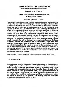
In this subsection, we consider the angular resolution obtained in a 3D arc diagram using straight-line edges drawn between vertices placed on a sphere. The two algorithms we present here are inspired by a two-dimensional drawing algorithm by Formann et al. [14]. Our main result is the following. Theorem 1. Let G = (V, E) be a graph of degree d. There is a 3D straight-line drawing of G with an angular resolution of Ω(1/d), with the vertices of G placed on the surface on a sphere. Proof. Let G2 = (V, E 2 ) be the square of G, that is the graph with the same set of vertices as G, and an edge between vertices (u, v) if there is a path of length ≤ 2 between u and v in G. Since G has degree d, G2 has degree ≤ d(d − 1) < d2 . Therefore, we can color the vertices of G2 with at most d2 colors, with the requirement that adjacent vertices have different colors. We place the vertices on a unit sphere S. We define d2 cluster positions as follows. First, we cut the circle with d + 1 uniformly spaced parallel planes (see Fig. 5), such that the maximum distance between the center of S and a plane is h (thus, the distance between two neighboring planes is 2h/d). Then, we uniformly place d points on each resulting circle. These are the cluster positions. Since a coloring C of G2 uses ≤ d2 colors, we can assign distinct cluster positions to colors in C. To obtain a drawing of G, we place all vertices of the same color in C on the sphere, S, within a small distance, , around this color’s cluster position, and draw edges in E as straight lines. We can remove any intersections by perturbing the vertices slightly. The claim is √ that the resulting drawing has resolution Ω(1/d). Indeed, by setting h = π/( 1 + π 2 ), we get Ω(1/d) minimal distance between any two planes, and Ω(1/d) minimal distance between any two cluster positions on the same plane. So, the distance between any two cluster positions is at least Ω(1/d). Now let us consider any angle ^abc formed by edges (a, b) and (b, c). The edges forming ^abc define a plane, P, whose intersection with S is a circle, C. _ Angle ^abc is inscribed in C, and based on the arc ac. Therefore, any other angle 7

Fig. 5. Sphere cut with equidistant planes. Red points are the cluster positions. _

inscribed in C and based on ac has the same size, in particular the one formed by an isosceles triangle 4adc. Since |ad| = |cd| ≤ 2 (S has radius 1), and |ac| is at least Ω(1/d), then |^abc| = |^adc| and is at least Ω(1/d). t u In addition, we also have the following. Corollary 1. Let G = (V, E) be a planar graph of degree d. There is a 3D straight-line drawing of G with an angular resolution of Ω(1/d1/2 ), with the vertices of G placed on the surface of a sphere. Proof. The proof is a direct consequence of applying the algorithm from the proof of Theorem 1 and the fact that the degree of G2 , the square of a planar graph, G, has degree O(d) [14]. t u Thus, we can produce 3D arc diagram drawings of planar graphs that achieve an angular resolution that is within a constant factor of optimal. Admittedly, this type of drawing is probably not going to be very pretty when rendered, say, as a video fly-through on a 2D screen, as this type of drawing is unlikely to project to a planar drawing in any direction. 4.2

Stationary Vertices

In this subsection, we show how to overcome the drawback of the above method, in that we show how to start with any existing 2D straight-line drawing and dramatically improve the angular resolution for that drawing using a 3D arc diagram rendering that projects perpendicularly to the 2D drawing. Theorem 2. Let D(G) be a straight-line drawing of a graph, G, with arbitrary, but distinct, placements for its vertices in the base plane. There is a 3D arc diagram drawing of G with the same vertex placements as D(G) and with an angular resolution at least Ω(1/d), where d is the degree of G, regardless of the angular resolution of D(G). 8

Proof. Since we are not allowed to move vertices, and edges have to lie on planes perpendicular to the base plane, we are restricted to selecting angles αe for edges e of G. We do it by utilizing classical edge coloring, observing that the “entry” and “exit” angles for each vertex need to match. First, we compute an edge coloring C of G with c colors (c ≤ d + 1). Then, for each edge e, if its color in C is i (i = 0, 1, . . . , c − 1), we set its angle to be αe = i · π/4(c − 1). For any two edges e1 , e2 , the difference between their angles αe1 and αe2 is at least π/4(c − 1) (let αe1 < αe2 ; consider the plane, P, determined by both tangent lines having angle αe1 ; the angle between e2 and the plane P, on which tangent of e1 lies, is αe2 − αe1 ). Therefore, by Lemma 2, the angle between e1 and e2 in the arc diagram is also at least π/4(c − 1) = Ω(1/d). It is unlikely that any pairs of the arcs touch each other in 3D, but if any pair of them do touch, we can perturb one of them slightly to eliminate the crossing, while still keeping the angular separation for every pair of incident edges to be Ω(1/d). t u In addition, through the use of a slanted 3D arc diagram rendering, we can produce a drawing with angular resolution that is within a constant factor of optimal, with each arc projecting to its corresponding straight-line edge in some direction. Theorem 3. Let D(G) be a straight-line drawing of a graph, G, with arbitrary, but distinct, placements for its vertices in the base plane. There is a slanted 3D arc diagram drawing of G with the same vertex placements as D(G) and with an angular resolution at least Ω(1/d1/2 ), where d is the degree of G, regardless of the angular resolution of D(G). Proof. Let C be a set of dd1/2 e + 1 uniformly distributed angles from 0 to π/4. Define a set of d + 1 “colors” as distinct pairs, (α, β), where α and β are each in C. Compute an edge coloring of G using these colors. Now let e be an edge in G, which is colored with (α, β). Draw the edge, e, using a circular arc that lies in a plane, P, that makes an angle of α with the base plane and which has a tangent in P that forms an angle of β at each endpoint of e. (For instance, in Fig. 1b, we give a slanted 3D arc diagram based on the edge coloring of the graph in Fig. 1a, corresponding to the following (αe , βe ) “colors:” (0◦ , 0◦ ), (22.5◦ , 0◦ ), (45◦ , 0◦ ), (22.5◦ , 22.5◦ ), (45◦ , 45◦ ).) The claim is that every pair of incident edges is separated by an angle of size at least Ω(1/d1/2 ). So suppose e and f are two edges incident on the same vertex, v. Let (αe , βe ) be the color of e and let (αf , βf ) be the color of f . Since e and f are incident and we computed a valid coloring for G, αe 6= αf or βe 6= βf . In either case, this implies that e and f are separated by an angle of size at least Ω(1/d1/2 ) (by Lemma 1 if βe = βf , by Lemma 2 otherwise), which establishes the claim. As previously, we can perturb the arcs to eliminate crossings in 3D. t u Thus, we can achieve optimal angular resolution in a 3D arc diagram for any graph, G, to within a constant factor, for any arbitrary placement of vertices of G 9

in the plane. Note, however, that even if D(G) is planar, the 3D arc diagram this algorithm produces, when projected to the base plane, may create edge crossings in the projected drawing. It would be nice, therefore, to have 3D arc diagrams that could have good angular resolution and also have planar perpendicular projections in the base plane. 4.3

Free Vertices

In this section, we show how to take any 2D straight-line drawing with good angular resolution and convert it to a 3D arc diagram with angular resolution that is within a constant factor of optimal. Moreover, this is the result that makes use of a localized edge coloring. Theorem 4. Let D(G) be a straight-line drawing of a graph, G, with arbitrary, but distinct, placement for its vertices in the base plane, and Ω(1/d) angular resolution. There is a 3D arc diagram drawing of G with the same vertex placements as D(G) and with angular resolution at least Ω(1/d1/2 ), where d is the degree of G, such that all arcs project perpendicularly as straight lines onto the base plane. Proof. The algorithm is similar to the one from the proof of Theorem 2. This time, however, we first compute an L-localized edge coloring, C, of G utilizing c colors (c ≤ 2L + 1). Then, as previously, we assign angle αe = i · π/4(c − 1) to an edge e of color i in C (i = 0, 1, . . . , c − 1). Let us consider two arcs, e and f , incident on a vertex, v. If αe 6= αf , then the angle between e and f is at least π/(4c) = Ω(1/L), by Lemma 2. Otherwise, αe = αf , and e and f have the same color in C. By the definition of L-localized edge coloring, e and f are separated by at least L/2 edges around v. Because D(G) has resolution Ω(1/d), the angle between e and f in D(G) is Ω(L/d). Thus, by Lemma 1, the angle between e and f is also Ω(L/d). Therefore, the angle between e and f is Ω(min{1/L, L/d}). We achieve the advertised angular resolution by setting L = d1/2 . t u Theorem 4 shows that we can achieve Ω(1/d1/2 ) angular resolution in a 3D arc diagram drawing of a graph, G, with arcs projecting perpendicularly onto the base plane as straight-line segments, if there is a straight-line drawing of G on a plane with an angular resolution of Ω(1/d). The following is an immediate consequence. Corollary 2. There is a 3D arc diagram drawing of any planar graph, G, with straight-line projection onto the base plane, and an angular resolution of Ω(1/d1/2 ). Proof. By [14], we can draw G in a straight-line manner on a plane with an angular resolution of Ω(1/d). t u Admittedly, the 2D projection of this graph is not necessarily planar. We can nevertheless also achieve the following. 10

Corollary 3. There is a 3D arc diagram drawing of any ordered tree, T , with straight-line projection onto the base plane, and an angular resolution of Ω(1/d1/2 ). Proof. By Duncan et al. [10], we can draw T in a straight-line manner on a plane with an angular resolution of Ω(1/d). t u In addition, the area of the projection of the drawings produced by the previous two corollaries is polynomial.

5

Conclusion

We have given efficient algorithms for drawing 3D arc diagrams that achieve polynomial area in the base plane or sphere that contains all the vertices while also achieving good angular resolution. Since our algorithms deal with arc intersections via arc perturbation, the results may not be satisfactory, as the perturbed edges will still be very close. Therefore, one direction for future work is a related resolution question of what volumes are achievable if, in addition to angular resolution, we also insist that every circular arc always be at least unit distance from every other non-incident arc edge.

Acknowledgements We thank Joe Simons, Michael Bannister, Lowell Trott, Will Devanny, and Roberto Tamassia for helpful discussions regarding angular resolution in 3D drawings.

References 1. P. Angelini, D. Eppstein, F. Frati, M. Kaufmann, S. Lazard, T. Mchedlidze, M. Teillaud, and A. Wolff. Universal point sets for planar graph drawings with circular arcs, 2013. manuscript. 2. U. Brandes. Hunting down Graph B. In J. Kratochv´ıyl, editor, Graph Drawing, volume 1731 of LNCS, pages 410–415. Springer, 1999. 3. U. Brandes, G. Shubina, and R. Tamassia. Improving angular resolution in visualizations of geographic networks. In W. Leeuw and R. Liere, editors, Data Visualization, Eurographics, pages 23–32. Springer, 2000. 4. U. Brandes, G. Shubina, and R. Tamassia. Improving angular resolution in visualizations of geographic networks. In Proc. Joint Eurographics — IEEE TCVG Symposium on Visualization (VisSym ’00), 2000. 5. C. Cheng, C. Duncan, M. Goodrich, and S. Kobourov. Drawing planar graphs with circular arcs. Discrete & Computational Geometry, 25(3):405–418, 2001. 6. A. Cimikowski and P. Shope. A neural-network algorithm for a graph layout problem. IEEE Trans. on Neural Networks, 7(2):341–345, 1996. 7. R. Cohen, P. Eades, T. Lin, and F. Ruskey. Three-dimensional graph drawing. Algorithmica, 17(2):199–208, 1997.

11

8. H. Djidjev and I. Vrto. An improved lower bound for crossing numbers. In P. Mutzel, M. J¨ unger, and S. Leipert, editors, Graph Drawing, volume 2265 of LNCS, pages 96–101. Springer, 2002. 9. C. A. Duncan, D. Eppstein, M. T. Goodrich, S. G. Kobourov, and M. L¨ offler. Planar and poly-arc Lombardi drawings. In M. Kreveld and B. Speckmann, editors, Graph Drawing, volume 7034 of LNCS, pages 308–319. Springer, 2012. 10. C. A. Duncan, D. Eppstein, M. T. Goodrich, S. G. Kobourov, and M. N¨ ollenburg. Drawing trees with perfect angular resolution and polynomial area. In U. Brandes and S. Cornelsen, editors, Graph Drawing, volume 6502 of LNCS, pages 183–194. Springer, 2011. 11. C. A. Duncan, D. Eppstein, M. T. Goodrich, S. G. Kobourov, and M. N¨ ollenburg. Lombardi drawings of graphs. In U. Brandes and S. Cornelsen, editors, Graph Drawing, volume 6502 of LNCS, pages 195–207. Springer, 2011. 12. D. Eppstein, M. L¨ offler, E. Mumford, and M. N¨ ollenburg. Optimal 3d angular resolution for low-degree graphs. In U. Brandes and S. Cornelsen, editors, Graph Drawing, volume 6502 of LNCS, pages 208–219. Springer Berlin Heidelberg, 2011. ¨ 13. L. Fejes T´ oth. Uber die Absch¨ atzung des k¨ urzesten Abstandes zweier Punkte eneis auf einer Kugelfl¨ ache liegenden Punktsystems. Jbf. Deutsch. Math. Verein, 53:66–68, 1943. 14. M. Formann, T. Hagerup, J. Haralambides, M. Kaufmann, F. T. Leighton, A. Symvonis, E. Welzl, and G. J. Woeginger. Drawing graphs in the plane with high resolution. In FOCS, pages 86–95. IEEE Computer Society, 1990. 15. A. Garg and R. Tamassia. Planar drawings and angular resolution: Algorithms and bounds. In J. van Leeuwen, editor, European Symp. on Algorithms (ESA), volume 855 of LNCS, pages 12–23. Springer, 1994. 16. A. Garg, R. Tamassia, and P. Vocca. Drawing with colors. In J. Diaz and M. Serna, editors, European Symp. on Algorithms (ESA), volume 1136 of LNCS, pages 12–26. Springer, 1996. 17. M. T. Goodrich and C. G. Wagner. A framework for drawing planar graphs with curves and polylines. Journal of Algorithms, 37(2):399–421, 2000. 18. C. Gutwenger and P. Mutzel. Planar polyline drawings with good angular resolution. In S. H. Whitesides, editor, Graph Drawing, volume 1547 of LNCS, pages 167–182. Springer, 1998. 19. T. Nicholson. Permutation procedure for minimising the number of crossings in a network. Proc. of the Inst. of Electrical Engineers, 115(1):21–26, 1968. 20. T. L. Saaty. The minimum number of intersections in complete graphs. Proceedings of the National Academy of Sciences of the United States of America, 52(3):688– 690, 1964. 21. P. Tammes. On the origin of number and arrangements of the places of exit on the surface of pollen grains. Rec. Trav. Bot. Neerl., 27:1–81, 1930. 22. V. G. Vizing. On an estimate of the chromatic class of a p-graph. Diskret. Analiz., 3:25–30, 1964. 23. M. Wattenberg. Arc diagrams: Visualizing structure in strings. In IEEE Symp. on Information Visualization (InfoVis), pages 110–116, 2002.

12