Graphics that made my career in computer graphics possible. When I left ...... The spatial resolution of a 17-inch 1280Ã1024 monitor, viewed from 24 inches, is 1.5 arcmin. This resolution is ...... debugging purposes on the laptop. 1280x800 ...
ACHIEVING NEAR-CORRECT FOCUS CUES USING MULTIPLE IMAGE PLANES
A DISSERTATION SUBMITTED TO THE DEPARTMENT OF ELECTRICAL ENGINEERING AND THE COMMITTEE ON GRADUATE STUDIES OF STANFORD UNIVERSITY IN PARTIAL FULFILLMENT OF THE REQUIREMENTS FOR THE DEGREE OF DOCTOR OF PHILOSOPHY
Kurt Akeley June 2004
c Copyright by Kurt Akeley 2004 � All Rights Reserved
ii
I certify that I have read this dissertation and that, in my opinion, it is fully adequate in scope and quality as a dissertation for the degree of Doctor of Philosophy.
Patrick Hanrahan (Principal Adviser)
I certify that I have read this dissertation and that, in my opinion, it is fully adequate in scope and quality as a dissertation for the degree of Doctor of Philosophy.
Martin S. Banks (Visual Space Perception Laboratory University of California, Berkeley)
I certify that I have read this dissertation and that, in my opinion, it is fully adequate in scope and quality as a dissertation for the degree of Doctor of Philosophy.
Mark A. Horowitz
Approved for the University Committee on Graduate Studies.
iii
Abstract Typical stereo displays stimulate incorrect focus cues because the light comes from a single surface. The consequences of incorrect focus cues include discomfort, difficulty perceiving the depth of stereo images, and incorrect perception of distance. This thesis describes a prototype stereo display comprising two independent volumetric displays. Each volumetric display is implemented with three image planes, which are fixed in position relative to the viewer, and are arranged so that the retinal image is the sum of light from three different focal distances. Scene geometry is rendered separately to the two fixed-viewpoint volumetric displays, using projections that are exact for each eye. Rendering is filtered in the depth dimension such that object radiance is apportioned to the two nearest image planes, in linear proportion based on reciprocal distance. Fixed-viewpoint volumetric displays with adequate depth resolution are shown to generate nearcorrect stimulation of focus cues. Depth filtering, which is necessary to avoid visible artifacts, also improves the accuracy of the stimulus that directs changes in the focus of the eye. Specifically, the stimulus generated by depth filtering an object whose simulated distance falls between image-plane distances closely matches the stimulus that would be generated by an image plane at the desired distance. Viewers of the prototype display required substantially less time to perceive the depth of stereo images that were rendered with depth filtering to approximate correct focal distance. Fixed-viewpoint volumetric displays are shown to be a potentially practical solution for virtual reality viewing. In addition to near-correct stimulation of focus cues, and unlike more familiar autostereoscopic volumetric displays, fixed-viewpoint volumetric displays retain important qualities of 3-D projective graphics. These include correct depiction of occlusions and reflections, utilization of modern graphics processor and 2-D display technology, and implementation of realistic fields of
iv
view and depths of field. The design and verification of the prototype display are fully described. While not a practical solution for general-purpose viewing, the prototype is a proof of concept and a platform for ongoing vision research.
v
Acknowledgement I have been blessed with wonderful parents, teachers, mentors, and colleagues. My parents, David and Marcy Akeley, inspired my appreciation of education, allowed me to disassemble the family car and washing machine, and brought our family together for thousands of evening meals where we shared the excitements of our day. Peter Warter, chairman of the University of Delaware electrical engineering department when I was an undergraduate there during the late 70’s, trusted me with project work at the graduate-student level, took me into his family, and encouraged me to attend graduate school at Stanford. James Clark, a new faculty member in the Stanford electrical engineering department when I met him in 1980, created the professional opportunities at Silicon Graphics that made my career in computer graphics possible. When I left Silicon Graphics after 20 years, Mark Horowitz and Pat Hanrahan made it possible for me to return to Stanford to complete my degree; and Martin Banks provided me with my thesis topic and the laboratory infrastructure at Berkeley in which much of the work was done. Without the support of all of these people this thesis would not have been possible. Many colleagues contributed directly to my thesis work. Simon Watt taught me the basics of vision-science experimental methods, and ran many of the experiments that are described in this thesis. Ahna Reza Girshick picked up where Simon left off, designing and running experiments that will be reported in future publications. Sergei Gepshtein improved my MATLAB proficiency with many useful tips and techniques. Ian Buck shared his deep knowledge of modern graphics systems with me, and set up the environment that allowed this old-time Unix user to run make and vi on his PC. Mike Cammarano helped to define the external image interface to the prototype software,
vi
and provided the ray traced images that are included in this thesis. And NVIDIA, my part-time employer, gave me the schedule flexibility I needed to get my thesis work done. My immediate family supported me emotionally, financially, and parentally throughout this work. Jian Zhao and Manli Wei, my parents-in-law, created an extended family that gave my children four parents, allowing me to spend many long days in the labs at Stanford and Berkeley. My deepest appreciation and love go to my wife, Jenny Zhao, and to my children, David and Scarlett. They gave me the freedom to go back to school, and the love and support that allowed me to enjoy every moment of it.
vii
Contents Abstract
iv
Acknowledgement
vi
1 Introduction
1
1.1
Related Work . . . . . . . . . . . . . . . . . . . . . . . . . . . . . . . . . . . . .
2
1.2
My Contribution . . . . . . . . . . . . . . . . . . . . . . . . . . . . . . . . . . .
4
2 Fixed-viewpoint Volumetric Display 2.1
2.2
2.3
6
Principles and Optimizations . . . . . . . . . . . . . . . . . . . . . . . . . . . . .
6
2.1.1
Non-homogeneous Voxel Distribution . . . . . . . . . . . . . . . . . . . .
8
2.1.2
Collapsing the Image Stack . . . . . . . . . . . . . . . . . . . . . . . . .
10
2.1.3
Solid-angle Filtering . . . . . . . . . . . . . . . . . . . . . . . . . . . . .
13
2.1.4
Reduced Depth Resolution . . . . . . . . . . . . . . . . . . . . . . . . . .
18
2.1.5
Wide Field of View . . . . . . . . . . . . . . . . . . . . . . . . . . . . . .
23
Attributes . . . . . . . . . . . . . . . . . . . . . . . . . . . . . . . . . . . . . . .
24
2.2.1
Tractable Voxel Count . . . . . . . . . . . . . . . . . . . . . . . . . . . .
24
2.2.2
Standard Components . . . . . . . . . . . . . . . . . . . . . . . . . . . .
25
2.2.3
Multiple Focal Distances . . . . . . . . . . . . . . . . . . . . . . . . . . .
25
2.2.4
No Eye Tracking . . . . . . . . . . . . . . . . . . . . . . . . . . . . . . .
27
Concerns . . . . . . . . . . . . . . . . . . . . . . . . . . . . . . . . . . . . . . .
29
2.3.1
29
Aperture-related Lighting Errors . . . . . . . . . . . . . . . . . . . . . . .
viii
2.3.2
Viewpoint Instability . . . . . . . . . . . . . . . . . . . . . . . . . . . . .
30
2.3.3
Silhouette Artifacts . . . . . . . . . . . . . . . . . . . . . . . . . . . . . .
32
2.3.4
Incorrect Retinal Focus Cues . . . . . . . . . . . . . . . . . . . . . . . . .
35
2.3.5
Head Mounting . . . . . . . . . . . . . . . . . . . . . . . . . . . . . . . .
35
3 Prototype Display
37
3.1
Design Decisions . . . . . . . . . . . . . . . . . . . . . . . . . . . . . . . . . . .
38
3.2
Implementation Details . . . . . . . . . . . . . . . . . . . . . . . . . . . . . . . .
41
3.2.1
Overlapping Fields of View . . . . . . . . . . . . . . . . . . . . . . . . .
41
3.2.2
Ergonomics . . . . . . . . . . . . . . . . . . . . . . . . . . . . . . . . . .
43
3.2.3
Software . . . . . . . . . . . . . . . . . . . . . . . . . . . . . . . . . . .
44
3.2.4
Construction . . . . . . . . . . . . . . . . . . . . . . . . . . . . . . . . .
46
Validation . . . . . . . . . . . . . . . . . . . . . . . . . . . . . . . . . . . . . . .
47
3.3.1
Intensity Constancy . . . . . . . . . . . . . . . . . . . . . . . . . . . . . .
48
3.3.2
Image Alignment . . . . . . . . . . . . . . . . . . . . . . . . . . . . . . .
49
3.3.3
Silhouette Visibility . . . . . . . . . . . . . . . . . . . . . . . . . . . . .
52
3.3.4
High-quality Imagery . . . . . . . . . . . . . . . . . . . . . . . . . . . . .
54
Issues . . . . . . . . . . . . . . . . . . . . . . . . . . . . . . . . . . . . . . . . .
56
3.3
3.4
4 User Performance
58
4.1
The Fuse Experiment . . . . . . . . . . . . . . . . . . . . . . . . . . . . . . . . .
58
4.2
Fuse Experiment Results . . . . . . . . . . . . . . . . . . . . . . . . . . . . . . .
61
4.3
Results Related to Analysis . . . . . . . . . . . . . . . . . . . . . . . . . . . . . .
63
5 Discussion and Future Work
69
A Apparent Focal Distance
73
B Blur Radius
78
C Incorrect Accommodation
81
ix
D Summed Images
90
E Dilated Pupil
98
F Software Configuration
104
G Design Drawings
139
H Prototype Display Specifications
147
I
149
Glossary
Bibliography
154
x
List of Tables 2.1
Box depth-filter discontinuity as a function of depth resolution. . . . . . . . . . . .
21
2.2
Relationship between vergence angle and fixation distance. . . . . . . . . . . . . .
28
3.1
Prototype image plane distances. . . . . . . . . . . . . . . . . . . . . . . . . . . .
40
D.1 ATF-sum maxima distances for various intensity ratios and spatial frequencies. . .
95
H.1 Prototype specifications. . . . . . . . . . . . . . . . . . . . . . . . . . . . . . . . 147 H.2 Prototype spatial resolution. . . . . . . . . . . . . . . . . . . . . . . . . . . . . . 148
xi
List of Figures 2.1
View dependent lighting effects. . . . . . . . . . . . . . . . . . . . . . . . . . . .
7
2.2
Actual and ideal linespread functions. . . . . . . . . . . . . . . . . . . . . . . . .
11
2.3
Modulation transfer functions of the actual and ideal linespread functions. . . . . .
11
2.4
Ideal display. . . . . . . . . . . . . . . . . . . . . . . . . . . . . . . . . . . . . .
12
2.5
Box filter shapes. . . . . . . . . . . . . . . . . . . . . . . . . . . . . . . . . . . .
14
2.6
Voxel lighting with box and tent depth filters. . . . . . . . . . . . . . . . . . . . .
16
2.7
Box and tent depth-filter shapes. . . . . . . . . . . . . . . . . . . . . . . . . . . .
18
2.8
Modeling the visual discontinuity due to box depth filtering. . . . . . . . . . . . .
19
2.9
Tent depth filtering eliminates visual discontinuities. . . . . . . . . . . . . . . . .
20
2.10 Multiple focal distances along a visual line. . . . . . . . . . . . . . . . . . . . . .
27
2.11 Alignment error due to optical center movement. . . . . . . . . . . . . . . . . . .
32
2.12 Intensity discontinuity at foreground/background transitions. . . . . . . . . . . . .
33
2.13 Intensity discontinuity due to voxel misalignment. . . . . . . . . . . . . . . . . . .
34
3.1
Four views of the prototype display. . . . . . . . . . . . . . . . . . . . . . . . . .
38
3.2
Prototype display layout schematic. . . . . . . . . . . . . . . . . . . . . . . . . .
39
3.3
Prototype field of view. . . . . . . . . . . . . . . . . . . . . . . . . . . . . . . . .
42
3.4
Depth filter functions for the three image depths. . . . . . . . . . . . . . . . . . .
45
3.5
Intensity constancy. . . . . . . . . . . . . . . . . . . . . . . . . . . . . . . . . . .
49
3.6
Horizontal alignment errors. . . . . . . . . . . . . . . . . . . . . . . . . . . . . .
51
3.7
Vertical alignment errors. . . . . . . . . . . . . . . . . . . . . . . . . . . . . . . .
52
3.8
Foreground and background silhouette texture images. . . . . . . . . . . . . . . .
53
xii
3.9
Example external left-eye and right-eye images. . . . . . . . . . . . . . . . . . . .
55
3.10 Full-screen image of the T221 flat panel. . . . . . . . . . . . . . . . . . . . . . . .
55
4.1
Fuse experiment, example scene geometries. . . . . . . . . . . . . . . . . . . . . .
59
4.2
Fuse experiment, full screen image. . . . . . . . . . . . . . . . . . . . . . . . . .
60
4.3
Fuse experiment, complete results. . . . . . . . . . . . . . . . . . . . . . . . . . .
61
4.4
Fuse experiment, mid and far fixation results. . . . . . . . . . . . . . . . . . . . .
62
4.5
Fuse experiment, mid, mid-far, and far fixation results. . . . . . . . . . . . . . . .
63
4.6
Fuse experiment, averaged subject performance. . . . . . . . . . . . . . . . . . . .
64
4.7
Fuse experiment, estimated image power spectra. . . . . . . . . . . . . . . . . . .
67
4.8
Fuse experiment, multiple spectra estimates. . . . . . . . . . . . . . . . . . . . . .
68
A.1 Convex and concave reflectors alter the focal distance. . . . . . . . . . . . . . . .
74
A.2 A cylindrical reflector has no focal point. . . . . . . . . . . . . . . . . . . . . . .
75
A.3 Detailed geometry of reflection off a spherical surface. . . . . . . . . . . . . . . .
77
B.1 Blur radius is proportional to focus error and aperture size. . . . . . . . . . . . . .
79
C.1 Geometry of the out-of-focus linespread computation. . . . . . . . . . . . . . . . .
82
C.2 Computed vs. exact linespread functions. . . . . . . . . . . . . . . . . . . . . . .
83
C.3 Out-of-focus linespread functions and their modulation transfer functions. . . . . .
86
C.4 Accommodative transfer function. . . . . . . . . . . . . . . . . . . . . . . . . . .
87
C.5 Computed vs. predicted modulation transfer functions. . . . . . . . . . . . . . . .
88
C.6 Computed vs. ideal modulation transfer functions. . . . . . . . . . . . . . . . . . .
89
D.1 Accommodative transfer function, 1/10-D separation, 3-mm pupil. . . . . . . . . .
92
D.2 Accommodative transfer function, 1/2-D separation, 3-mm pupil. . . . . . . . . . .
93
D.3 Maximum image plane separations that avoid ATF-sum inversion, 3-mm pupil. . .
94
D.4 Real-world and summed-image retinal blur gradient, 3-mm pupil. . . . . . . . . .
96
E.1 Approximated linespread function, 6-mm pupil. . . . . . . . . . . . . . . . . . . .
99
E.2 Accommodative transfer functions, 3-mm and 6-mm pupils. . . . . . . . . . . . . 100 xiii
E.3 Maximum image plane separations that avoid ATF-sum inversion, 3-mm and 6-mm pupils. . . . . . . . . . . . . . . . . . . . . . . . . . . . . . . . . . . . . . . . . . 101 E.4 Accommodative transfer function, 1/10-D separation, 6-mm pupil. . . . . . . . . . 102 E.5 Accommodative transfer function, 1/2-D separation, 6-mm pupil. . . . . . . . . . . 103 G.1 Mirror box, side view. . . . . . . . . . . . . . . . . . . . . . . . . . . . . . . . . . 140 G.2 Mirror box, front view. . . . . . . . . . . . . . . . . . . . . . . . . . . . . . . . . 141 G.3 Mirror box, top view. . . . . . . . . . . . . . . . . . . . . . . . . . . . . . . . . . 142 G.4 Bite bar mount, front and top views. . . . . . . . . . . . . . . . . . . . . . . . . . 143 G.5 Periscope assembly, front view. . . . . . . . . . . . . . . . . . . . . . . . . . . . . 144 G.6 Periscope slider assembly, front and top views. . . . . . . . . . . . . . . . . . . . 145 G.7 Periscope prism mount and miscellaneous components. . . . . . . . . . . . . . . . 146
xiv
Chapter 1
Introduction Fred Brooks has observed that “VR barely works” [8]. Problems such as excessive system latency, inadequate image resolution, and bounded scene complexity limit the utility of today’s virtualreality (VR) systems. Various techniques, including in particular application of the exponential increase in performance of 3-D rendering hardware [3], are being used to address these problems. There are few remaining limitations that are not on such an improvement track. Chief among those is the lack of correct stimulation of focus cues. The human visual system is well adapted to its natural environment. Eye movements and the focusing of the eyes normally work together. Vergence eye movements change the angular difference between the eyes’ visual axes. This angular difference determines the location of the fixation point, where the visual axes intersect. Accommodation, the focus response of the eye, determines the focal distance of the eye. In natural vision accommodative distance and the distance to the fixation point are coupled [14]. The coupling is broken while viewing typical stereo graphics displays, which provide correct binocular disparity, specifying a range of fixation distances, while forcing accommodation to a single image plane. Consequences of the forced decoupling of viewer vergence and accommodation include discomfort [54], induced binocular stress [27, 48], and difficulty perceiving the depth relationships specified by binocular disparities [48]. Another consequence of this decoupling is error in the perception of scene geometry. Estimation of distance in scene geometry is more accurate, for example,
1
CHAPTER 1. INTRODUCTION
2
when correct focal distance information is provided than when correct binocular projections of an object are viewed at the wrong accommodative distance [50]. Accommodation to a single image plane also eliminates a depth cue—variation in retinal blur—and this too causes error in the perception of scene geometry [24]. This thesis proposes a new display technique—fixed-viewpoint volumetric—as an approach to the correct stimulation of focus cues. My long-term goal is to enable augmented reality with practical head-mounted display technology, so that viewers experience direct views merged with generated graphics in day-to-day settings. Achieving this goal requires high image quality, image correctness, and viewer comfort. To determine whether fixed-viewpoint volumetric displays offer a path toward this long-term goal, I implemented a prototype display. The prototype was designed as a test bed for the proposed approach to display design, and also to support further vision research. It is not practical for day-to-day use. Chapter 2 describes the principles of fixed-viewpoint volumetric displays, identifies optimizations that may be employed by practical implementations, and address potential concerns. Chapter 3 describes the hardware and software implementation of the prototype display, the validation of its basic operation, and some of its limitations. Chapter 4 describes a study of user performance done with the prototype. The appendixes include analysis of retinal blur under various conditions: reflection from a non-planar surface, incorrect accommodation, and accommodation to the same image presented at multiple focal distances. Use of the prototype display for further vision research will be presented in other technical papers.
1.1
Related Work
Other investigators have sought solutions to the issue of incorrect focus cues. From as early as the Mercury and Gemini space programs, out-the-window displays for vehicle simulation systems have fixed the focal distance at infinity by collimating the light from the display [29]. A similar effect is achieved by positioning the display surface sufficiently far from the viewer. Infinite focal distance is a good approximation because out-the-window displays depict only the scene beyond the vehicle itself—the vehicle interior is implemented as a physical model. Such physical modeling
CHAPTER 1. INTRODUCTION
3
is inappropriate for virtual reality systems, which render all aspects of the visible scene based on retained and computed geometry. Infinity optics is not a suitable solution for general-purpose VR systems. Autostereoscopic volumetric displays, which present scene illumination to multiple viewpoints as a volume of light sources (voxels), naturally provide correct disparity and stimulation of focal cues. However, these displays do not create true light fields. While the inability of voxels to occlude each other is sometimes given as the reason for this limitation [34], the problem is actually more fundamental: voxels emit light of the same color in all directions, so neither view-dependent lighting effects nor occlusions can be represented simultaneously for multiple viewing positions. A volumetric display could in principle be implemented with directional voxels, such that the perceived color of each voxel varied depending on the viewpoint. The directional resolution required to correctly stimulate focus cues is enormous, however, so such a display will not be practical in the foreseeable future [39]. Autostereoscopic volumetric displays are typically small because they are designed to be viewed from various angles and because of the high expense of larger voxel volumes. These displays suffer other practical difficulties, which result from the huge increase in voxels that follows the introduction of a generalized third dimension to the display. Because conventional display technology cannot be leveraged to satisfy this resolution requirement, autostereoscopic volumetric displays either compromise resolution or implement custom image-generation approaches, such as laser stimulation of doped media as described by Downing et al. [10]. Two commercial products, Perspecta [11, 2] and DepthCube [42, 20], compromise resolution in different ways. Both products use DLP projection [37] to illuminate individual planes of voxels. Perspecta displays 100 million voxels in a spherical volume. Frame rate is limited to 30 Hz, and pixel color resolution is limited to approximately four bits per color component.1 DepthCube implements only 20 planes of voxels, which are organized in the depth dimension by limiting the viewing angle of the display. Luminance-modulation displays present a single viewer with images at two distinct depths, both projected to the viewer’s cyclopean eye [43, 44]. Because the projections are not correct for either eye, view-dependent lighting and occlusion effects are compromised much as they are 1
I computed this value based on the data in Sampsell et al. [37] and in the Perspecta data sheet [2].
CHAPTER 1. INTRODUCTION
4
in autostereoscopic volumetric displays. Binocular disparities, which are displayed correctly in volumetric displays, are also incorrect. Non-volumetric approaches to the correct stimulation of focus cues are also possible. One approach adjusts the focal distance of the entire display to match the viewer’s accommodative distance [33], which is estimated by tracking gaze direction or vergence angle. Displays that adjust focal distance on a per-pixel basis, based on known scene geometry and independent of viewer accommodation, have also been implemented [40, 25]. A significant limitation of these approaches is that they cannot present multiple focal distances along a visual line (Section 2.2.3). Holographic displays with sufficiently high resolution automatically stimulate correct focus cues. But, as is the case with directional voxels, achieving the required resolution is not currently possible, given the computational and optical requirements [32, 22, 23]. This thesis closely follows the work of two other groups of investigators. Rolland et al. computed the spatial and depth resolution requirements for a multi-plane, head-mounted display, as part of an overall feasibility study [36]. They suggested several possible design approaches, including volumetric display technology, but no implementation or results were presented. McDowall and Bolas augmented the Fakespace Boom product with prism assemblies such that image planes at two focal distances were summed. Their work was not published, however, and no studies of its effectiveness were ever performed. Neither Rolland et al. nor McDowall and Bolas considered depth filtering, which is related to the luminance-modulation function of Suyama et al. and is a key feature of the fixed-viewpoint, volumetric approach to display that is presented in this thesis. The importance of depth filtering is described in Section 2.1.3, and its implementation is described in Section 3.2.3.
1.2
My Contribution
Martin Banks and Mike Landy proposed a multi-plane display that would utilize dynamic optics to me in 2000, while I was the chief technology officer of Silicon Graphics. After my return to Stanford as a Ph.D. candidate I agreed to collaborate with Martin to further develop this concept.
CHAPTER 1. INTRODUCTION
5
We applied for NIH support in September of 2001. The work described in this thesis is in partial fulfillment of the resulting NIH grant, award number R01 EY14194-01. I developed the principles of fixed-viewpoint volumetric displays that are described in Chapter 2, including in particular the importance of continuous filtering in the depth dimension (depth filtering). I conceived of the single-LCD, multi-beamsplitter approach to implementation that is described in Chapter 3. I designed and constructed three prototype displays, the third of which is described in this thesis. I designed and implemented the software that controls these displays, including the algorithm for depth filtering. I designed and implemented the procedures that were used to calibrate the prototype display. I conceived of and implemented the experiments that were used to validate its performance and utility. (I collaborated with others to design these experiments.) And I did the theoretical work on accommodation that is described in Appendixes A, B, C, D, and E. Specific contributions of the thesis are: • Development of the rationale for a new type of display—fixed-viewpoint volumetric—with analysis of potential shortcomings. • Design of a laboratory-quality prototype display, comprising two fixed-viewpoint volumetric subsystems, each implemented with depth filtering. • Experimental demonstration that user performance is not compromised when fixation distances are simulated with images at two focal distances, using the technology of depth filtering. • Analytic demonstration that depth filtering improves the accuracy of the stimulus to accommodation, for spatial frequencies below a limit determined by the dioptric distance between image planes and the pupil diameter of the eye.
Chapter 2
Fixed-viewpoint Volumetric Display Existing displays have various combinations of strengths and weaknesses, but none deliver highquality images and correct focus cues. This chapter introduces fixed-viewpoint volumetric display, a combination of display methodologies that results in high-quality stereo images with near-correct stimulation of focus cues. The principles and optimizations that characterize a fixed-viewpoint volumetric display are developed in Section 2.1. The attributes that make fixed-viewpoint volumetric displays desirable are identified and described in Section 2.2. Finally, Section 2.3 begins the exploration of potential shortcomings and limitations, which is continued in subsequent chapters.
2.1
Principles and Optimizations
Fixed-viewpoint volumetric displays derive most directly from autostereoscopic volumetric displays, which inherently stimulate correct focus cues. In addition to practical limitations, however, autostereoscopic volumetric displays are fundamentally unable to generate correct view-dependent lighting effects for multiple simultaneous view points. Such effects include reflection, specularity (the preferential scattering of light around the angle of reflection), and occlusion (the suppression of light that is blocked from the viewpoint). Because autostereoscopic volumetric displays do not have these abilities, objects displayed using them appear to be fully transparent, never opaque or partially-opaque, and they show no highlights or reflections. This is unacceptable in almost all applications. 6
CHAPTER 2. FIXED-VIEWPOINT VOLUMETRIC DISPLAY
7
This limitation is the direct result of the nature of the voxels that compose volumetric displays. An individual voxel is non-directional—it emits light of the same color and intensity in all directions. So voxels look the same from all directions, eliminating the possibility of view-dependent effects for multiple simultaneous views, as depicted in Figure 2.1. For a single fixed view position, however, a volumetric display can provide completely correct view-dependent lighting effects. Used in this manner, voxels that are occluded from the view position are dark, and voxel intensity is chosen to correctly represent view-dependent lighting along visual lines. A fixed-viewpoint volumetric display is a non-autostereoscopic volumetric display, with rendering that is correct for its single fixed view position.
Light Point D Viewer A
Viewer B
Viewer C
Figure 2.1: View dependent lighting effects. Viewers A and B both see point D, but viewer A sees diffuse illumination, while viewer B sees the specular reflection of the light. Point D is occluded along viewer C’s line of sight, so it is not visible at all. Because a fixed-viewpoint volumetric display supports only one viewing position, a stereoscopic implementation must have two independent fixed-viewpoint volumetric displays. The added expense and complexity are more than offset, however, by optimizations that are made possible by fixing the viewing position relative to the display. These optimizations, 1. Non-homogeneous voxel distribution,
CHAPTER 2. FIXED-VIEWPOINT VOLUMETRIC DISPLAY
8
2. Collapsing the image stack, 3. Solid-angle filtering 4. Reduced depth resolution, and 5. Full field of view are detailed in the following subsections.
2.1.1
Non-homogeneous Voxel Distribution
A volumetric display is a 3-dimensional volume of non-directional, non-occluding light sources called voxels. The Cartesian and cylindrical voxel distributions that are typical of autostereoscopic volumetric displays [10, 11, 20] are not optimal for a display with a single fixed viewing position. An optimal voxel distribution is instead dictated by the spatial and focus resolutions of the human eye. The maximum resolvable spatial frequency of a human subject is 60 cycles/deg (cpd). This resolution is achieved only along the visual axis, for signals projected on the fovea [46]. In a typical configuration the display will be rigidly connected to the viewer’s head, so view direction will be limited by the range of motion of the eye. This range is approximately 100 deg horizontally and 90 deg vertically [7], but viewers typically limit eye rotations to 20 deg from center, rotating their heads to achieve larger changes [41, 4]. An ideal display would satisfy the need for 60-cpd visual resolution over the required 40-deg field of view, and provide a coarser resolution over the remaining 160×135-deg field of view of the eye. Section 2.1.5 addresses full field of view as a separate optimization. Except in that section, this thesis treats as ideal a display comprising image planes with 50-deg fields of view, each centered about the visual axis of the unrotated eye. To satisfy the Nyquist limit, voxel density on an image plane must be at least twice that of the 60-cpd maximum spatial frequency, or 120 voxels/deg. If voxels are spaced regularly on an image plane, as is desirable for simplicity in rendering, then the lowest apparent voxel density occurs at the center of the image plane, since this location is nearest to the eye and is viewed at the least oblique angle (90 deg). The voxel dimensions of an ideal image
CHAPTER 2. FIXED-VIEWPOINT VOLUMETRIC DISPLAY
9
plane are 6,400×6,400, each dimension being twice the ratio of the half-width of the image plane (at distance r) and the width of the centermost pixel: 6, 400 = 2
r tan 25 r tan 1/120
(2.1)
. Display resolution in the depth dimension affects only focus cues. While the human eye’s ability to resolve different distances using only focus cues has not been quantified as accurately as its maximum resolvable spatial frequency, it is possible to estimate the required depth resolution. The focus error of an optical system is the difference between the distance to the object and the distance to which the system is focused. Focus error is typically quantified in units of reciprocal distance, such as diopters (1 / meters), rather than in units of metric distance. The derivation in Appendix B shows that, in an ideal optical system, the out-of-focus image of a point light source is a disk whose radius is proportional to focus error measured in diopters. This suggests that the depth resolution of a fixed-viewpoint volumetric display should be distributed linearly in dioptric units, rather than metric units, to keep focus error constant throughout the range of displayed depths. If the optics of the human eye were ideal, a point light source would become visibly blurred when the diameter of the defocused image disk exceeded the spacing of receptors in the fovea. Equation B.5, which defines disk radius (θ) in arcmin as a function of pupil radius (ra ) and focus error (e), can be rewritten to express focus error as a function of pupil radius and blur disk radius: e=
tan θ . ra
(2.2)
Substituting 1/4 arcmin (half the 1/2-arcmin foveal receptor spacing [46]) and 0.0015 m (half the typical 3-mm pupil diameter) into Equation 2.2 gives a maximum focus error of 1/20 diopter (D). This maximum would be satisfied by image planes separated by 1/10 D, because focus could always be to the nearer image plane.
CHAPTER 2. FIXED-VIEWPOINT VOLUMETRIC DISPLAY
10
The optics of the eye are not ideal, however. Figures 2.2 and 2.3 illustrate that the inherent blur of the eye is greater than the blur of an ideal optical system that is defocused by 1/6 D.1 The solid plot in Figure 2.2 is the cross-section of the retinal image of an ideal line light source, viewed by a correctly focused eye with a 3-mm pupil aperture. The image of the line is many arcmin wide, greatly exceeding the 1/2-arcmin separations of the retinal receptors. Because the image of a correctly-focused point light source is similarly blurred, the determination of when such a light source becomes visibly defocused is not as simple as the treatment in the previous paragraph suggests. Based on their assessment of visual acuity, Rolland et al. [36] estimated the required spacing of image planes as 1/7 D. This thesis takes as ideal a voxel depth resolution of 1/7 D.
The range of human accommodation is at most 8 D [46]. A display with the full accommodative range, and a depth resolution of 1/7 D, requires 56 image planes. Diopters bunch near the eye (Figure 2.4), so moving the near-field limit of the display slightly away from the viewer greatly reduces the accommodative range of the display. The 4-D range from 1/4 m (10 inches) to infinity requires only 28 image planes, for example, and is treated as ideal in this thesis because it satisfies most viewing situations (Figure 2.4). The voxel depth of such a 4-D-range display is more than two orders of magnitude lower than the 6,400-voxel spatial dimensions of an ideal image plane. Fixing the position of the viewpoint allows a dramatic reduction in voxel count with no reduction in image quality.
2.1.2
Collapsing the Image Stack
As described thus far the ideal fixed-viewpoint volumetric display has a manageable depth resolution of 28 voxels, but it is too large to be implemented as part of a head-mounted display. Each image plane is centered in its focal range, so the farthest plane is 1/14 D from infinity, or 14 m from the viewpoint. At least two approaches to collapsing the physical depth of the image plane stack, while maintaining the focal distance relationships, have been proposed. 1
The inherent blur of the eye serves the useful purpose of pre-filtering, eliminating aliasing and probably increasing vernier acuity. It is non-ideal only in the sense of absolute imaging quality.
CHAPTER 2. FIXED-VIEWPOINT VOLUMETRIC DISPLAY
11
Relative intensity
1 Westheimer '86, 3-mm Ideal, 3-mm, 1/6-D error
0.5
0 -10
-8
-6
-4
-2
0
2
4
6
8
10
Visual angle (arcmin) Figure 2.2: Actual and ideal linespread functions. The solid plot is the cross-section of the retinal image of a line light source through a 3-mm pupil, as modeled by Westheimer [52]. The dotted plot is the image of the same line through an ideal optical system (no diffraction, no aberration) with a 3-mm aperture and a focus error of 1/6 D. The modulation transfer functions of the two linespread functions (Figure 2.3) show that the inherent blur of the eye is greater than the 1/6-D blur of the ideal optical system.
Amplitude scale factor
1.2 Westheimer '86, 3-mm Ideal, 3-mm, 1/6-D error
1.0 0.8 0.6 0.4 0.2 0 -0.2 -0.4 0
10
20
30
40
50
60
Spatial frequency (cpd) Figure 2.3: Modulation transfer functions of the actual and ideal linespread functions. These functions were computed by convolving the linespread functions of Figure 2.2 with sine waves of various frequencies, then plotting the resulting amplitudes. The 1/6-D-defocused ideal optical system has lower attenuation for all frequencies below 47 cpd.
CHAPTER 2. FIXED-VIEWPOINT VOLUMETRIC DISPLAY
12
6,400 voxels 1/14 D
14 m 50 deg
3/14 D
4.67 m
5/14 D
2.80 m
55/14 D
0.25 m
Figure 2.4: Ideal display. Twenty-eight image planes at 1/7-D separations form the display that is regarded as ideal in this thesis. Each image plane has 6,400×6,400 voxel dimensions, insuring a minimum spatial resolution of 1/2 arcmin, measured at the center of the 50-deg field of view. One solution uses dynamic optics to sequentially position a single image plane at multiple focal distances. An oscillating lens can be used for this purpose. Adaptation of the adaptive-optics technology used in large telescopes is also possible. Both approaches have the advantage of requiring only one image plane, and also result naturally in near-optimal spatial distribution of voxels. Time multiplexing images at separate focal distances introduces difficulties, however, including: • Motion artifacts. The approach of rendering a view once, then using retained depth information to sequentially generate and display images at different focal distance, will create visible artifacts related to viewer and object motion. To avoid these artifacts, images that are displayed sequentially must also be rendered at the correct sequential time steps, so the rendering frame rate must be increased to match the display frame rate. • Inter-frame cross talk. Ghosts of images at incorrect focal distances will be visible if the display response time is greater than the duration of a single frame. Few display technologies have response times low enough to support frame rates that are integer factors of 60 Hz.
CHAPTER 2. FIXED-VIEWPOINT VOLUMETRIC DISPLAY
13
• Slow optics. If the dynamic optics are not instantaneous, but are fast enough to stabilize in significantly less than a frame period, then pixels may be displayed only while the optics are stable. The resulting duty cycle further reduces the acceptable display response time, and reduces the available intensity of the display. • Magnification distortion. If, as is more likely, the dynamic optics are adjusted continuously, then pixels must be illuminated during adaptation. Because adaptive optics cannot be located at the optical center of the viewer’s eye, changes in focal distance generate corresponding changes in magnification.2 If optics adaptation is continuous, individual pixels must be illuminated for very short periods of time, or change in magnification displacement during illumination will create the effect of short pixel paths. If pixels are themselves illuminated sequentially, as they are in common cathode-ray tube (CRT) displays, then rendered images must be warped to compensate for the different magnification displacements of individual pixels. The other solution, suggested by Rolland et al. [36], retains the stack of image planes and requires no moving parts or time multiplexing. Instead, individual transparent image planes are viewed through a fixed positive lens. When an n-D lens is placed close to the eye, the focal distance of an image plane at infinity is preserved by moving it n diopters closer to the eye. The physical depth of the resulting image plane stack is approximately 1 m n + (1/14)
(2.3)
in the case of the ideal display.
2.1.3
Solid-angle Filtering
The axis-aligned voxel filtering that is typical of renderings for volumetric displays is not suitable for a display with a single fixed viewing position. This is illustrated most clearly by considering the shapes that box filters form around voxel centers. The left panel of Figure 2.5 illustrates a small 2
Magnification is a function of the optical power and of the position of a lens placed in front of the eye [13].
CHAPTER 2. FIXED-VIEWPOINT VOLUMETRIC DISPLAY
14
portion of a 2-D slice of voxels. The slice is taken from a 3-D Cartesian array of voxels, arranged as they would be in an autostereoscopic volumetric display. The shaded region defines the box filter of the voxel it encloses. Objects within the region contribute equally to the color and intensity that are assigned to the voxel during rasterization. Objects outside the region have no influence on the voxel’s color or intensity. The boundaries of the region are axis-aligned—they are parallel to the axes of the voxel array. This is true in the third dimension as well. (The box filter is actually a cube, centered around the voxel center.) Because the voxels in the 3-D array are regularly spaced, the shapes and alignments of the box filters surrounding each voxel are identical.
Autostereoscopic
Fixed-viewpoint
Figure 2.5: Box filter shapes. The left panel shows a box filter in a 2-D slice of an autostereoscopic display. The box filter in the right panel is aligned with visual lines that pass through the fixed viewpoint. (Voxels are not to scale.) The right panel of Figure 2.5 illustrates the very different shapes of the box filters in a fixedviewpoint volumetric display. Again the shaded region defines the box filter of the voxel it encloses. The near and far boundaries of this region are axis aligned. But the left and right boundaries are
CHAPTER 2. FIXED-VIEWPOINT VOLUMETRIC DISPLAY
15
projection-aligned—they are coincident with visual lines rather than the axes of the voxel array. This is true in the third dimension as well. (The box filter is actually a frustum, roughly centered around the voxel.) I will refer to this filtering as solid-angle filtering to distinguish it from the axis-aligned filtering used when rendering to autostereoscopic volumetric displays. Box filters make good expository devices, but not good images. Spatial filtering may be improved through the use of Gaussian, Mitchell [26], or other filters. The regions of these filters are larger than the region of a box filter, and objects within a region contribute to the final pixel value in relation to their locations, rather than equally. Consider the rasterization of a scene to a single image plane, as is done when 3-D geometry is rendered to a screen. For reasons of efficiency the spatial filter typically operates on samples, rather than on a continuous representation of the geometry, which may be extremely difficult to compute. A sample represents the light that reaches the eye along a single visual line. Color intensity is computed independently for each sample, based on the intersections of the sample’s visual line with the geometry of the scene. The spatial filter computes the pixel color and intensity as a weighted sum of the sample values, with weights corresponding to the locations of the samples within the filter function. This algorithm is called multisample antialiasing. Solid-angle filtering is best implemented as an extension to multisample antialiasing. The depth filter is applied during the computation of each sample, based on the apparent focal distance of the light source.3 If multiple light sources contribute to the light along a single visual line, each is depth filtered separately, then they are summed to form the sample value. When the samples are complete the spatial filter is applied to compute the final voxel value. Spatial filter quality is more important for fixed-viewpoint volumetric displays than for traditional displays, for reasons that are discussed in Section 2.3.3. But higher spatial resolution reduces the need for spatial antialiasing, just as it does for traditional displays. Single-sample (aliased) rasterization produces a usable result if the spatial resolution of the display approaches the ideal defined in Section 2.1.1. 3 Appendix A explains how apparent focal distance is determined. For light reflected from a diffuse surface it is the distance to that surface. Other cases are more complex.
CHAPTER 2. FIXED-VIEWPOINT VOLUMETRIC DISPLAY
16
Spatial filter quality is important, but depth-filter quality is crucial for fixed-viewpoint volumetric displays. If a box filter is used, rasterized voxels are either on or off, with respect to the intensity of a rendered object. This binary behavior introduces discontinuities in the voxel volume that do not exist in the rendered objects themselves. The human visual system is optimized to detect such discontinuities, which cannot be eliminated even with perfect alignment and calibration of the display.
Box depth filter
Tent depth filter Out-of-focus image plane In-focus image plane
Figure 2.6: Voxel lighting with box and tent depth filters. The black bars on the image planes represent regions of lighted voxels that result from the rendering of the object surface that is positioned between the image planes. Box filtering results in a discontinuity of intensity, while tent filtering does not. The left panel of Figure 2.6 illustrates such a case, using a simplified fixed-viewpoint volumetric display with only two image planes. The object is a surface that is rotated slightly away from frontoparallel orientation. Regions of lighted voxels are indicated by the heavy black bars on each of the image planes. The in-focus image plane is lighted where the object surface is closer to it than it is to the out-of-focus image plane. (Equivalently, where the object surface intersects the box
CHAPTER 2. FIXED-VIEWPOINT VOLUMETRIC DISPLAY
17
filter frustums of the voxels of the in-focus image plane.) Likewise voxels in the out-of-focus image plane are lighted where they are closer to the object. The discontinuity occurs where the image energy moves instantaneously from the in-focus image plane to the out-of-focus image plane. If the location of the object changes from frame to frame, the discontinuity moves as well. Motion increases the distraction that the discontinuity creates, and may also increase its visibility.4 Figure 2.8 illustrates why this discontinuity is visible, even if the voxels in the display are perfectly aligned. Voxels are modeled to subtend 1 arcmin, a realistic resolution that is half the ideal. The focus error of the out-of-focus voxels is modeled as 1/2 D, corresponding to a display with the relatively coarse depth resolution of 2 voxels / diopter. The light from the individual voxels is integrated into a retinal image, taking into account the imperfect optics of the human eye. The result is a discontinuity with an absolute magnitude of 32% of the amplitude of the signal. This discontinuity is obviously visible—it is large not only in absolute value, but also when compared with the discontinuities that result from the light distribution patterns of the individual voxels. Using a tent depth filter completely eliminates the discontinuity. Figure 2.7 illustrates how weights are assigned to samples that fall within a tent filter. The right panel of Figure 2.6 illustrates the assignment of voxel intensity when a tent filter is used. (Increased darkness of the bars corresponds to increased voxel intensity.) Figure 2.9 illustrates the computation of the retinal signal in this case, again taking the focus error of the out-of-focus voxels to be 1/2 D. There is no discontinuity larger than those due to the individual voxels themselves. How closely spaced must the image planes be for there to be no visible discontinuity when depth filtering is implemented using a box filter? While this figure can be established with certainty only by experimentation, modeling can be used to develop an estimate. Presumably a display with high depth resolution would also have high spatial resolution, so voxels subtend 1/2 arcmin in this new model. Table 2.1 lists the focus errors for which the new model was run, and the absolute sizes of the discontinuities that resulted. 4
Contrast sensitivity increases as modulation frequency is increased from zero to 8 Hz [49].
CHAPTER 2. FIXED-VIEWPOINT VOLUMETRIC DISPLAY
18
Box filter
Tent filter
Figure 2.7: Box and tent depth-filter shapes. Box filters are binary. They assign full value to samples that fall within them, and no value to other samples. The tent filter weights sample values based on how close they are to the center of the tent. Tent filters overlap such that the sum of the weights assigned to any sample is always 1.0. An instantaneous 2% change in luminance is the smallest perceptible under optimum conditions [6]. All of the depth resolutions listed in the table exceed this magnitude of discontinuity, suggesting that the depth resolution at which the discontinuity is no longer visible is much greater than 7 voxels/diopter (the ideal determined in Section 2.1.1). Depth filtering using a continuous filter function is required for all fixed-viewpoint volumetric displays with practical depth resolutions.
2.1.4
Reduced Depth Resolution
Depth filtering is required to avoid visible artifacts. But depth filtering accomplishes more than the elimination of artifacts—it changes the way that focus cues are stimulated by the display. The 1/7-D depth-resolution requirement computed in Section 2.1.1 assumed accommodation to a single image
CHAPTER 2. FIXED-VIEWPOINT VOLUMETRIC DISPLAY
In-focus Signal Intensity
1
-15
Relative intensity
-5 0 5 10 Visual angle (arcmin)
-15
1.5
-10
-5 0 5 10 Visual angle (arcmin)
In-focus Retinal Image
-15
-10
-5 0 5 10 Visual angle (arcmin)
Intensity
1.5
15
-5 0 5 10 Visual angle (arcmin)
15
Out-of-focus Linespread Function
-15
1.5
0.5
-10
0.5
0
15
1
0
-15
1
0.5
0
1
0
15
In-focus Linespread Function
1
Intensity
-10
Relative intensity
0
Out-of-focus Signal (1/2 D)
2
Intensity
Intensity
2
19
-10
-5 0 5 10 Visual angle (arcmin)
15
Out-of-focus Retinal Image
1 0.5 0
-15
-10
-5 0 5 10 Visual angle (arcmin)
15
Composite Retinal Image
1 0.5 0
-15
-10
-5 0 5 10 Visual angle (arcmin)
15
Figure 2.8: Modeling the visual discontinuity due to box depth filtering. This figure is based on the scene in the left panel of Figure 2.6 (Box Depth Filter). Voxels occlude 1 arcmin, and each has an intensity distribution equivalent to one half of a sine wave. The in-focus and out-of-focus voxel light distributions are plotted in the upper-left and upper-right graphs, based on application of a box depth filter. The in-focus and 1/2-D out-of-focus linespread functions show how light from a line source is spread across the retina. They are developed in Appendix D. Convolving the linespread functions with the corresponding signal images results in the in-focus and out-of-focus retinal images. The sum of these two retinal images has a large discontinuity.
CHAPTER 2. FIXED-VIEWPOINT VOLUMETRIC DISPLAY
In-focus Signal Intensity
1
-15
Relative intensity
-5 0 5 10 Visual angle (arcmin)
-15
1.5
-10
-5 0 5 10 Visual angle (arcmin)
In-focus Retinal Image
-15
-10
-5 0 5 10 Visual angle (arcmin)
Intensity
1.5
15
-5 0 5 10 Visual angle (arcmin)
15
Out-of-focus Linespread Function
-15
1.5
0.5
-10
0.5
0
15
1
0
-15
1
0.5
0
1
0
15
In-focus Linespread Function
1
Intensity
-10
Relative intensity
0
Out-of-focus Signal (1/2 D)
2
Intensity
Intensity
2
20
-10
-5 0 5 10 Visual angle (arcmin)
15
Out-of-focus Retinal Image
1 0.5 0
-15
-10
-5 0 5 10 Visual angle (arcmin)
15
Composite Retinal Image
1 0.5 0
-15
-10
-5 0 5 10 Visual angle (arcmin)
15
Figure 2.9: Tent depth filtering eliminates visual discontinuities. This figure is based on the scene in the right panel of Figure 2.6 (Tent Depth Filter). Voxels occlude 1 arcmin, and each has an intensity distribution equivalent to one half of a sine wave. The in-focus and out-of-focus voxel light distributions are plotted in the upper-left and upper-right graphs, based on tent depth-filter application as illustrated in Figure 2.7. The in-focus and 1/2-D out-of-focus linespread functions show how light from a line source is spread across the retina. They are developed in Appendix D. Convolving the linespread functions with the corresponding signal images results in the in-focus and out-of-focus retinal images. The sum of these two retinal images shows no discontinuity.
CHAPTER 2. FIXED-VIEWPOINT VOLUMETRIC DISPLAY
Voxels/diopter 2 3 4 5 6 7 8 9 10 11 12 13 14 15
Focus error 0.500D 0.333D 0.250D 0.200D 0.167D 0.143D 0.125D 0.111D 0.100D 0.091D 0.083D 0.077D 0.071D 0.067D
21
Discontinuity 31.9% 22.3% 16.4% 12.4% 9.8% 7.9% 6.4% 5.3% 4.5% 3.9% 3.3% 2.9% 2.6% 2.3%
Table 2.1: Box depth-filter discontinuity as a function of depth resolution. Voxels are arranged as in Figure 2.6, each voxel subtending the optimal 1/2 arcmin. The two image planes are separated by focus error diopters, corresponding to a display system with depth resolution voxels/diopter. With the eye focused on the nearer image plane, the retinal image of the scene has a discontinuity with the magnitude listed in the third column, as a percentage of the average image intensity. Figure 2.8 illustrates a retinal image much like that corresponding to the first row of this table, except that the voxels in that figure subtend 1 arcmin. plane. In a depth-filtered display the eye typically accommodates to the sum of light from two adjacent image planes. Both retinal and extra-retinal focus cues are affected by this design decision. Discussion of retinal focus cues is deferred to Section 2.3.4. The extra-retinal focus cue is the sequence of muscle commands that control the accommodative response of the eye. The dynamics of the extra-retinal focus cue are affected by the coupling of accommodation to vergence [14], as discussed in Chapter 1. Ultimately, however, this cue is determined by an automatic process that maximizes high-frequency content in the foveal image. The analysis in Appendix D demonstrates that the high-frequency content of the foveal image of the sum of two image planes is maximized, not by accommodation to the focal distance of either plane, but instead by accommodation to an intermediate distance that is determined by the relative intensities of the images. Thus, for the purpose of stimulating the extra-retinal cue, depth
CHAPTER 2. FIXED-VIEWPOINT VOLUMETRIC DISPLAY
22
filtering greatly increases the effective depth resolution of a fixed-viewpoint volumetric display. This increase can be exploited to increase the spacing of the image planes. Image-plane spacing remains constrained, however. The increase in depth resolution is effective only for spatial frequencies below a maximum that is determined by the separation of the image planes and by the viewer’s pupil diameter. Figure D.3 plots maximum image plane separation as a function of the maximum spatial frequency for which the effect is enabled, for a typical pupil diameter of 3 mm. If spatial frequencies through 60 cpd are to be maximized during accommodation, the image plane separation can be no larger than 1/7 D, and thus no reduction in depth resolution is possible. If the maximum frequency is relaxed to 30 cpd, however, image plane separation can be increased slightly beyond 1/4 D. Separations of 1/2 D become possible for maximum spatial frequencies just under 20 cpd. Two factors can be used to argue for relaxing the maximum frequency constraint: 1. Low visibility. High spatial frequencies are strongly attenuated by the optics of the eye, as illustrated in Figure 2.3. Spatial frequencies above 40 cpd are visible only under ideal conditions [5, 46]. And contrast sensitivity limitations make minor variations in high-frequency signals invisible. Thus frequencies above 30 cpd or 40 cpd may have no effect on accommodation. 2. Coupling. Figure D.3 plots the maximum image-plane separation for a foveal image that is, in principle, sufficiently-correct to stimulate correct accommodation during monocular viewing. Because accommodation is coupled to vergence, however, the visual system strongly favors accommodation to the fixation distance during stereo viewing. Thus, in a stereo display utilizing depth filtering, the characteristics of the foveal image need only be sufficient to avoid disrupting the natural coupling. These factors are not definitive, but they suggest that depth resolution may be reduced significantly below the 1/7-D limit established in Section 2.1.1, without stimulating incorrect extra-retinal focus cues.
CHAPTER 2. FIXED-VIEWPOINT VOLUMETRIC DISPLAY
2.1.5
23
Wide Field of View
Because the viewer of an autostereoscopic display cannot typically be inside the display, such displays are best used for non-immersive, sometimes called outside-in, tasks [28]. Fixed-viewpoint volumetric displays move with the viewer, however, so they do not divide space into static occupied and viewable volumes. They can be used effectively for both outside-in and immersive (inside-out) applications. The visual cues that are stimulated by a full field of view are known to be important in immersive applications [45]. The monocular visual field, measured from central fixation, is 160-deg wide and 135-deg high [46]. With 20-deg eye rotation in any direction, the required field of view approaches 180 deg. While extending the field of view to this range could add significant expense to a display, several optimizations are possible. Among these are: 1. Reduced resolution. The density of photopic receptors in the periphery is about 1/20 that of the foveal density [47]. Voxels used to extend the field of view beyond the 50-deg subtended by the ideal image planes could have substantially lower spatial resolution. 2. Inclined planes of projection. If image planes were used to extend the field of view, these planes could be angled to maximize apparent resolution near the 50-deg central image planes. To do this, they would be inclined such that visual lines at the extreme periphery were perpendicular to the planes. 3. Single focal distance. Given the low retinal resolution and poor optical quality of vision in the periphery, it is not obvious that focus cues are significant in the extended field of view. If not, a single surface of voxels in the periphery would be sufficient. Using rendering techniques (not physical adjustment) the multi-plane central image could be smoothly transitioned to a single plane at its boundary to avoid visual discontinuities.
CHAPTER 2. FIXED-VIEWPOINT VOLUMETRIC DISPLAY
2.2
24
Attributes
The fixed-viewpoint volumetric approach to display is a potentially practical solution to the shortcomings of current displays. Several of its desirable attributes are described in the following subsections.
2.2.1
Tractable Voxel Count
Traditional autostereoscopic volumetric displays have equivalent resolution requirements in all dimensions, because they can be viewed from all directions. A fixed-viewpoint volumetric display requires orders of magnitude less resolution in the depth dimension, however, giving it a substantial implementation advantage. With spatial voxel dimensions of roughly 6,400, and a depth dimension of 28, an ideal fixed-viewpoint volumetric display requires 1.15 billion voxels, making it impractical for the near future. But a useful display can be implemented with less than ideal resolution. The spatial resolution of a 17-inch 1280×1024 monitor, viewed from 24 inches, is 1.5 arcmin. This resolution is typical of current personal computer systems. The nVision Datavisor HiRes head-mounted display has a spatial resolution of 1.9 arcmin [31], which is typical of high-end headmounted displays. So the 1/2-arcmin resolution of the ideal fixed-viewpoint volumetric display is three to four times better than current practice. Relaxing this resolution to 1.5 arcmin reduces the voxel count by an order of magnitude (3 × 3 � 10). Similar reduction may be possible in the depth dimension, as described in Section 2.1.4. Chapter 4 provides evidence that the focus cue stimulation provided by the prototype display, which implements image planes with 2/3-D separations, significantly improved subject performance. At these spatial and depth resolutions a 4-D depth range requires six image planes. A more conservative 1/2-D image-plane separation increases the requirement to eight image planes. With these reductions the total voxel count of a fixed-viewpoint volumetric display falls to approximately 32 million. This is a small multiple of the nearly 10 million pixels available on today’s highest-end display systems [55]. By reducing the voxel penalty of providing near-correct stimulation of focus cues to as little as a factor of six, fixed-viewpoint volumetric displays allow the possibility of practical implementation.
CHAPTER 2. FIXED-VIEWPOINT VOLUMETRIC DISPLAY
2.2.2
25
Standard Components
The prototype display that is described in Chapter 3 is constructed using readily-available graphics and display hardware. This is possible because: • The required voxel count is moderate, for the reasons outlined in Section 2.2.1. • The only special requirement of the voxels is that they be non-occluding. In particular, they need not, and should not, be directional light sources. • The required voxel distribution, which strongly emphasizes spatial resolution over depth resolution, favors implementation using a sparse stack of 2-D image surfaces. This allows implementation using existing planar display and rendering hardware. Advanced fixed-viewpoint volumetric displays will make more demands of their components, but they may continue to utilize standard components, or to utilize technology that is developed for such components. So the billions of dollars that are being spent developing graphics processor and 2-D display technology will directly benefit the development of fixed-viewpoint volumetric displays.
2.2.3
Multiple Focal Distances
Automatic computation of a summed-intensity projection, such as is desired when viewing volumetric medical images, is an often-claimed advantage of autostereoscopic volumetric displays. While this viewing techniques is important, the feature is actually a deficiency, because it cannot be disabled while retaining multi-viewpoint viewing. It is an optical rendering technique—important aspects of the image are created by the display itself. But rendering is better implemented and controlled using the software and hardware algorithms that have been evolved over the past few decades. A summed-intensity projection can be rendered into a frame buffer to produce the same effect as is generated automatically by an autostereoscopic volumetric display. Other desirable projections, such as the maximum-value projection that is commonly used with medical imaging, cannot be optically computed by a volumetric display, yet these too can be rendered easily.
CHAPTER 2. FIXED-VIEWPOINT VOLUMETRIC DISPLAY
26
In a fixed-viewpoint volumetric display, the additive nature of light along a visual line is not used to compute a general summed-intensity projection. Instead, this capability supports depth filtering, as described in Section 2.1.3, and also allows for multiple focal distances along a single visual line. The need for multiple focal distances along a visual line is not as widely appreciated as the need for multiple focal distances in different visual directions. The left panel in Figure 2.10 illustrates an example of this need. The surface of the cube scatters light (from a matte component of the surface) and reflects light (from a glossy component). Because the cube’s surface is flat, the correct focal distance of the reflection of the (diffuse) cylinder is the sum of the distances from the eye to the cube and from the cube to the cylinder.5 The correct focal distance of the scattered light is the distance from the eye to the cube. The right panel of Figure 2.10 illustrates how this scene is rendered into a fixed-viewpoint volumetric display. The reflection is drawn deeper into the display, at the focal distance that is the sum of the eye-to-cube and cube-to-cylinder distances. Fixed-viewpoint volumetric displays also vary their spatial stimulation of focus cues in a nearcorrect manner. A significant strength of the visual system is that objects that are much nearer or farther than the fixation point are blurred. Such objects cannot be fused, because their disparity is too great, so blurring has the desirable effect of de-emphasizing them. If the focal distance of the entire display is uniformly adjusted to match the fixation distance, as is the case with some display techniques [33, 36], then all objects in the scene are in focus, even those that cannot be fused.6 Another shortcoming of displays that uniformly adjust focal distance is that slight changes in gaze can cause significant and distracting changes throughout the field of view. Displays that uniformly adjust focal distance are unable to display multiple focal distances along a single visual line. Even displays that adjust focal distance on a per-pixel basis often lack the ability to display multiple focal distances at a single pixel [25, 40]. Only holographic displays match fixedviewpoint volumetric displays in this ability, but their capability is theoretical, because holographic displays with the required resolution are not available. 5
If the reflecting surface is not planar the reflected light typically spans a range of focal distances. Appendix A provides some details. 6 Omura et al. [33] stimulate near-correct retinal focus cues by blurring the displayed image as a function of pixel depth.
CHAPTER 2. FIXED-VIEWPOINT VOLUMETRIC DISPLAY
Scene geometry
27
Volumetric illumination
Figure 2.10: Multiple focal distances along a visual line. The reflection of the cylinder has a longer focal distance than the surface of the cube. The right panel illustrates how the scene in the left panel is rendered to a volumetric display with high depth resolution. Subtractive image planes, such as stacked LCD flat panels, cannot directly implement a true volumetric display. Both depth filtering and multiple-focal-distance rendering depend on summing light along visual lines, which is possible only when voxels are additive light sources. Even perpixel adjustment of focal distance may not be possible in subtractive displays. Because depth filtering cannot be done, sharp discontinuities in depth would result from per-pixel adjustment of focal distance. These discontinuities would be much more visible than the similar discontinuities in additive displays, because direct illumination from the back-light would become visible.
2.2.4
No Eye Tracking
View position, the position and orientation of the viewer’s head, must be tracked for correct rendering to a fixed-viewpoint volumetric display. But view direction, the orientation of the eyes in
CHAPTER 2. FIXED-VIEWPOINT VOLUMETRIC DISPLAY
28
the head, has no consequence, because the display correctly depicts the entire field of view. Displays that uniformly adjust focal distance to match the viewer’s accommodation must somehow measure it. Because accommodation and vergence are coupled [14], accommodation can be measured directly or inferred from the gaze directions of the eyes. Directly measuring accommodation is possible, but is difficult to do without interfering with the viewer. Inferring accommodation from gaze directions can be done by either computing the fixation distance, based on the vergence angle, or by determining what is being observed, based on the gaze angles and knowledge of the scene geometry. In either approach the determination of the gaze angles is critical. Table 2.2 lists vergence angles for various fixation distances, demonstrating that the relationship between vergence angle and fixation distance is nearly linear—roughly 3.4 deg/D. Because the rotations of both eyes are measured to compute vergence, measurement errors of just 1/8 deg result in 1/7-D errors in focal distance, the threshold of visibility.
Distance ∞ 1.000 meters 0.500 meters 0.333 meters 0.250 meters 0.200 meters 0.167 meters 0.143 meters 0.125 meters
Diopters 0D 1D 2D 3D 4D 5D 6D 7D 8D
Vergence 0.00 deg 3.44 deg 6.87 deg 10.29 deg 13.69 deg 17.06 deg 20.41 deg 23.72 deg 26.99 deg
�vergence 3.44 deg 3.43 deg 3.42 deg 3.40 deg 3.37 deg 3.35 deg 3.31 deg 3.27 deg
Table 2.2: The relationship between vergence angle and fixation distance is nearly linear—roughly 3.4 deg/D. Fixation is directly ahead of the viewer. The precision required to correctly determine fixation distance by intersecting the visual axes with the scene geometry cannot be computed exactly, because scene depth changes instantaneously. Some insight is gained, however, by observing that a 1/8-deg error at 2 meters is 4 mm, a small but significant lateral error in a complex scene.
CHAPTER 2. FIXED-VIEWPOINT VOLUMETRIC DISPLAY
2.3
29
Concerns
This section discusses five concerns that derive from the properties and attributes that characterize a fixed-viewpoint volumetric display. The concerns that can be resolved are considered first. Those remaining are introduced, and are considered further in subsequent chapters.
2.3.1
Aperture-related Lighting Errors
A central concept of this thesis is that a volumetric display can correctly represent view-dependent lighting effects for a single view point. But the eye does not have a single view point; it collects light through an aperture (the pupil) and focuses this light on the retina. Indeed, if this were not the case, there would be no need for correct focus cues. How serious is this problem, and what can be done about it? Two factors mitigate the importance of differences in lighting across the eye’s aperture. First, the aperture is small, specifically in comparison to the separation between the eyes. Pupil diameter ranges from one to eight millimeters [46]; the typical value is approximately 3 mm. Interocular distance (IOD), the center-to-center separation of the eyes, is approximately 60 mm [46]. So the separation of the eyes is typically 20 times greater than the diameters of the eyes’ apertures. Lighting effects that clearly differ from one eye to the other may differ insignificantly within the aperture of a single eye. Second, and more fundamental, the light that is collected through the pupil is integrated to form a single image, not interpreted as separate images. As a result the visual system is not equipped to distinguish lighting differences across the pupil, as it is for differences between the eyes. The problem is minor, but an improvement can be had with moderate effort. If fixation is at a voxel, then the voxel is correctly lighted by double integrating the view-dependent lighting across the area of the pupil and the solid angle of the voxel.7 If fixation is far from a voxel, then a small error in its intensity or color is insignificant, because the voxel is out of focus, viewed in the eye’s periphery, or both. So a good approach is to render each voxel as though it was the fixation point, 7
Because the voxel is in focus, there is no difference between integrating the true light field across the area of the pupil, as the eye does when it views the actual scene, and integrating a precomputed average value, as the eye does when it views a voxel of this intensity and color.
CHAPTER 2. FIXED-VIEWPOINT VOLUMETRIC DISPLAY
30
assuming a typical pupil diameter. Such rendering is correct where it matters most (when it is near the fixation point), and errs only slightly otherwise. Spatial filtering is equivalent to a single integration across the solid angle of the voxel. The computational cost of doubling the integration to include sampling the area of the pupil may be lower than expected, because the number of samples required is similar to the number required to perform either integration separately [12]. Spatial filtering and aperture sampling are coupled— given suitable rendering hardware, either both or neither may be implemented.
2.3.2
Viewpoint Instability
Section 2.2.4 argues that fixed-viewpoint volumetric displays do not require eye tracking, because only eye position, not gaze direction, is important. But the optical center of the eye moves slightly as the eye rotates, so it is not rigid with respect to the viewer’s head. A display that assumes such rigidity will render incorrectly. The optical center of the eye lies on the visual axis approximately 5.7 mm ahead of the eye’s center of rotation [15]. When eye movements are limited to a maximum rotation of 20 deg, as is assumed in this thesis, the locust of the optical center is a disk 3 mm in diameter. With extreme eye rotations, such as the range used in Section 2.1.1 to compute ideal display resolution, the locus diameter reaches 8 mm. The severity of the problem can be gauged by evaluating the resulting alignment errors. Figure 2.11 illustrates the error calculation for an eye rotation of r deg, with voxel surfaces 1/n and 1/f diopters from the view point. Object A, a tiny sphere, is rendered to a view point at the optical center of the unrotated eye, lighting voxels at An and Af . Rotating the eye moves the visual axis d = 0.0057 sin r
(2.4)
meters from the initial optical center. When viewed by the rotated eye, voxel An is aligned with voxel Bf , rather than with voxel Af . The distance between Af and Bf is related to d, n, and f by similar triangles: e=d
f −n . n
(2.5)
CHAPTER 2. FIXED-VIEWPOINT VOLUMETRIC DISPLAY
31
Because e is small, the angle it subtends is its ratio to the circumference of the surface, converted to arcmin: earcmin = (360)(60)
e . 2πf
(2.6)
Substituting Equations 2.4 and 2.5 into 2.6 gives the alignment error in arcmin as a function of the rotation of the eye and of distances n and f : earcmin = 19.6 sin r
f −n . nf
(2.7)
Because 1 1 f −n ≡ − , nf n f Equation 2.7 can be rewritten as earcmin = 19.6s sin r s=
1 n
− f1 .
(2.8)
The alignment error depends on the dioptric separation of the display surfaces; it is independent of their absolute distances. Any alignment error is bad, but errors that cause double images due to solid-angle filtering, as illustrated in Figure 2.11, are pernicious. Substituting 20 deg (the maximum eye rotation) and 1/2 D (a large surface separation) into Equation 2.8 gives an alignment error or 3.5 arcmin. This error is seven times the desired spatial display resolution, and is significantly greater than the resolution of currently practical displays. Thus an object will look like two separate objects, rather than a single object with light coming from two distances, when it is viewed directly. The solution proposed in Section 2.3.1—rendering each voxel as though it was the fixation point—also addresses the problem of optical-center movement. The location of the optical center is known for a given fixation, and solid-angle filtering done to this view point results in exact alignments under fixation. Voxels in the periphery will be incorrectly aligned, but errors of a few arcmin are not visible in the periphery, where the receptor spacing exceeds 2 arcmin [47].
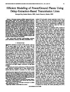
CHAPTER 2. FIXED-VIEWPOINT VOLUMETRIC DISPLAY
32
e=d Bf
(f-n) n
Af
A
Radius f An
Radius n Optical center (initial)
Optical center (rotated) 0.0057
r
Center of rotation
d = 0.0057 sin r Figure 2.11: Alignment error due to optical center movement. Object A is rendered to a view point at the unrotated optical center of the eye, lighting voxels at An and Af . Alignment error e results when the display is viewed with the eye rotated r deg. Distances are in meters. The eye’s center of rotation is on the visual axis, just 5.7 mm from the optical center. So rendering using the center of rotation as the view point is almost identical to rendering each voxel using the adjusted optical center as the view point. Because hardware rendering systems typically assume a single view point, using the center of rotation is a good optimization.
2.3.3
Silhouette Artifacts
Figure 2.8 in Section 2.1.3 illustrates how intensity discontinuities in depth become visible to an observer with finite depth of field. Solid angle filtering with a continuous depth filter eliminates these discontinuities where they result from poor depth filtering. But what about depth discontinuities that derive from the scene itself? Figure 2.12 illustrates such a discontinuity. The foreground object occludes the background object, so the farther image plane is unlighted on visual lines that extend through the lighted region
CHAPTER 2. FIXED-VIEWPOINT VOLUMETRIC DISPLAY
33
of the nearer image plane. If the rendered colors of the foreground and background objects are identical, there should be no visible discontinuity at the silhouette. But a visible discontinuity is expected for two reasons: 1. The geometry of the lighting is identical to that of Figure 2.8, which results in visible discontinuity for viewers with finite depth of field, and 2. The voxels in the two image planes may not subtend the same angular regions.
Background object Farther image plane Nearer image plane Foreground object
Figure 2.12: Intensity discontinuity at foreground/background transitions. The black bars on the image planes represent regions of lighted voxels that result from rendering the foreground and background objects. Problem (2) is the result of practical display design issues. In an ideal display the voxels of each image surface subtend identical visual angles. But such exact alignment is unlikely in real display systems, which utilize components that were not designed exclusively for fixed-viewpoint volumetric displays, and compensate for minor registration errors by altering rendering parameters
CHAPTER 2. FIXED-VIEWPOINT VOLUMETRIC DISPLAY
34
rather than making physical adjustments. Figure 2.13 shows, with artificially low resolution, how gaps and overlaps in illumination up to one voxel in width result from aliased rendering, where each voxel is lighted based on a single point sample along a ray that passes through the voxel center. Improved spatial sampling, as discussed in Section 2.1.3, largely eliminates this problem by assigning voxel illumination based on percentage of coverage, rather than on the basis of a single sample.
Background object Farther image plane Nearer image plane Foreground object
Figure 2.13: Intensity discontinuity due to voxel misalignment. At the left silhouette edge there is an overlap in illumination of almost a full voxel. At the right silhouette edge there is a 1/2 voxel gap. I know of no solution to problem (1), which is fundamental. Fortunately a visible discontinuity at a silhouette is less objectionable than a discontinuity within a smooth surface. The silhouette is a discontinuity, and identical shading of foreground and background objects is unlikely. When the object shading differs, the discontinuity due to depth of focus may be dwarfed by the difference in color, and by effects due to chromatic error in the eyes.
CHAPTER 2. FIXED-VIEWPOINT VOLUMETRIC DISPLAY
2.3.4
35
Incorrect Retinal Focus Cues
In Section 2.1.4 I argued that depth resolution can be reduced below the 1/7-D limit without stimulating incorrect extra-retinal focus cues. This argument deferred the discussion of retinal focus cues. Retinal focus cues derive from the image that is projected across the entire retina. Retinal images of objects at focal distances that differ substantially from the accommodative distance of the viewer are blurred, providing a discrete variation in blur. An object surface that is inclined toward the viewer produces a retinal image with a continuous variation in blur—blur gradient. Both discrete and continuous change in blur are retinal focus cues. Discrete differences in focal distance that are large, relative to the separations of the image planes, are depicted accurately by fixed-viewpoint volumetric displays. Blur gradients, however, are not accurately depicted, especially for focal distances between those of the image planes that bound the current accommodative distance. The analysis in Appendix D demonstrates that blur gradients around the accommodative distance are strongly affected by small changes in accommodation. When accommodation is to the dioptric midpoint between two image planes, for example, there is no change in blur throughout the focal distances bounded by those planes. (Because the image planes are equally defocused, redistributions of their intensities that result from depth filtering have no effect on the retinal image of their sum.) As accommodation moves toward one of the image planes local blur gradient increases, reaching an approximation of the correct gradient only when accommodation is to an exact image plane focal distance. The dependence of blur gradient on accommodative distance is fundamental to a depth-filtered display. Unlike the silhouette problem, however, for which there is no solution, blur gradients improve as depth resolution is increased. Thus any requirement for blur gradient quality can be transformed into a required minimum depth resolution.
2.3.5
Head Mounting
Because fixed-viewpoint volumetric displays require viewer position to be fixed with respect to the display, practical display systems must be head mounted. But head-mounted display systems are mechanically awkward, and their use in conjunction with high-latency image generators and
CHAPTER 2. FIXED-VIEWPOINT VOLUMETRIC DISPLAY
36
poor quality head tracking has resulted in user dissatisfaction and low adoption. Because head mounting is required to achieve augmented reality and the integration of image generation into everyday life, however, I expect continued engineering efforts that will successfully address current limitations. Latency, for example, is being reduced steadily due to increases in rendering frame rate [3] and improvements in tracking technology [1]. And 2-D display technology is evolving at an unprecedented rate.
Chapter 3
Prototype Display Three stereo, fixed-viewpoint volumetric displays were designed and implemented as part of this research effort. The first two were functional, and building them helped me to improve my construction techniques and to validate, or correct, various design decisions. But they were not suitable for the laboratory environment in which the formal validation and user studies were performed. These displays are not described further in this thesis, except for a brief mention in Appendix G. The third display, shown in four views in Figure 3.1, is the subject of this chapter. It is a prototype, in that its appearance is distinctly utilitarian, it is not practical for day-to-day use, and it has other significant shortcomings that are identified in Section 3.4. But its spatial and depth resolutions are high enough, and its alignment and intensity accuracies good enough, that it served as a laboratory test bed for the utility of the fixed-viewpoint volumetric approach to display. I will refer to this display as the prototype display for the remainder of this thesis. Sections 3.1 and 3.2 describe the design and implementation of the prototype display. This design suited our purposes, but it is just one example of many possible approaches. It is important to distinguish the fixed-viewpoint volumetric display approach, which is defined in Chapter 2, from the design decisions made for the prototype display. The prototype display utilizes beamsplitters, for example, but beamsplitters are not fundamental to fixed-viewpoint volumetric displays.
37
CHAPTER 3. PROTOTYPE DISPLAY
38
Figure 3.1: Four views of the prototype display. The T221 flat panel is removed in the bottom two images to expose the beamsplitters and front-surface mirrors.
3.1
Design Decisions
The design of the prototype display required compromises, which were reached after consideration of the project priorities. My primary goal was to determine the viability of an optimized fixed-viewpoint volumetric stereo display. I felt that depth resolution was the most important consideration. The design had to provide several image planes at substantially different focal distances, and these planes had to be additive so that depth filtering could be implemented. Stereo capability with significant overlap of the view frusta was also critical. And the display had to provide good laboratory ergonomics, so that many subjects could be tested with repeatable results.
CHAPTER 3. PROTOTYPE DISPLAY
39
A general design guideline emphasized visual quality over quantity. Thus high spatial resolution was important, but depth of field, field of view, frame rate, and latency were relatively unimportant, as long as they were sufficient to support the required testing. Ease of implementation was also a factor. For example, although motion parallax is an important cue, I felt that the difficulty of implementing a head-mounted display, which would require collapsing the image stack and tracking viewing position and orientation, outweighed the benefit. And spatial resolution, while much greater in the prototype display than in earlier versions, was still compromised in the interest of simplified implementation (Table 3.1). Figure 3.2 depicts the optical paths of the prototype display. An LCD flat panel is viewed through plate beamsplitters such that each eye sees three superimposed images. The use of a single flat panel limits the physical dimensions of the prototype display, and thus the available depth range and field of view, but it also has significant advantages.
IBM T221 flat panel
Figure 3.2: Prototype display layout schematic. Each eye views three superimposed viewports. Periscope optics separate the visual axes so that the left and right viewports do not overlap on the flat panel.
CHAPTER 3. PROTOTYPE DISPLAY
40
Pixel locations are precise because they are fixed by the manufacturer of the LCD flat panel in a regular grid. The digital interface is used to drive the LCD flat panel, so there is no drift in the relationship of the pixels in the frame buffer to those on the panel surface. Thus the locations of the six rendered viewports are known exactly, can be changed precisely and reliably, are coplanar, and cannot become rotated or skewed with respect to each other. The LCD flat panel is driven by a single graphics card, avoiding synchronization and other system complexities associated with multiple graphics cards.
Name Near Mid Far
Distance 0.311 m 0.394 m 0.536 m
Diopters 3.21 D 2.54 D 1.87 D
�D 0.67 D 0.67 D
Spatial resolution 1.38 arcmin 1.09 arcmin 0.80 arcmin
Table 3.1: Prototype image plane distances. Because no optical elements other than beamsplitters and mirrors are used, the focal distances of the three image planes are equal to their metric distances (Table 3.1). The 2/3-D separations of the image planes are wide compared with the 1/7-D separations of the ideal display. This spacing tests the effectiveness of depth filtering, and was driven by my concern for adequate vertical field of view, which would have been reduced from the current +/-4.4 deg had the spacing been tightened. The horizontal fields of view are 6.1 deg outside and 12.6 deg inside. The IBM T221 LCD flat panel [55], with a linear pixel density of 80/cm, is currently the highest resolution device of its kind on the market. The flat panel dimensions are 0.478×0.299 m, with an overall resolution of 3840×2400 pixels. Because the viewports are viewed at different distances, angular spatial resolution differs for the near, mid, and far viewports (Table 3.1). Even the nearviewport resolution was high enough that observers did not comment on the visibility of individual pixels. The LCD flat panel is driven by a 128MB NVIDIA Quadro 900 XGL graphics card, manufactured by PNY technologies [30]. This card has enough on-board memory to support the 9-Mpixel flat panel with 32-bit double-buffered color and a 24-bit Z-buffer, and to store the required texture images. Rendering performance is more than adequate, but because only two DVI display ports are
CHAPTER 3. PROTOTYPE DISPLAY
41
available, the display frame rate is limited to 12 Hz at full 3840×2400 resolution. This low frame rate is acceptable because LCD flat panels do not flicker. LCD flat panels cannot switch quickly enough to be viewed through shutter glasses. This, along with the low display frame rate, forced the decision to implement the stereo views with nonoverlapping viewports. (I also preferred the non-overlapping approach to time-multiplexed displays for image-quality reasons.) The aluminum periscope assembly that separates the left-eye and righteye visual axes is visible in Figure 3.1. The arrangement of the viewports and the paths of the visual axes are illustrated in Figure 3.2, and example images are provided in Figures 3.9 and 3.10.
3.2
Implementation Details
3.2.1
Overlapping Fields of View
The mirror box is divided into left and right rectangular chambers, one for each eye. Each chamber supports two beamsplitters and one front-surface mirror. Viewed from above, the chambers are 14 inches long, roughly matching the height of the T221 display, which rests above them facing down. The availability of 7×5 inch mirrors and beamsplitters1 determined the 7-inch chamber widths. The separations of the beamsplitters and the mirror were chosen to avoid view path interference and to be equal in units of diopters. What remained was to choose where the visual axes would enter the chambers. The periscopes bend light at right angles, causing the visual axes to be parallel to the long sides of the chambers (Figure 3.2). There is no reason for the vertical field of view to be asymmetric, so the visual axes are centered vertically (Figure G.1). Symmetric horizontal fields of view, however, would result in relatively little overlap of the left and right view frusta. Instead, I chose to offset each visual axis horizontally by 1/2 of the interocular distance (IOD). The resulting fields of view, as well as those that would have resulted from symmetric arrangement, are illustrated in Figure 3.3. The IOD-offset overlap is significantly larger, especially as it intersects the near and mid image planes (heavy lines in Figure 3.3). 1
Edmund Industrial Optics stock numbers NT40-043 (front surface mirror), NT43-362 (plate beamsplitter 30R/70T), and NT61-260 (plate beamsplitter 40R/60T).
CHAPTER 3. PROTOTYPE DISPLAY
42
Symmetric
IOD offset Far
Mid Near
Figure 3.3: Prototype field of view. The left panel illustrates symmetric fields of view, and the relatively small overlap that would result. The right panel illustrates the fields of view that result from the 1/2-IOD horizontal offsets of the visual axes, as implemented by the prototype display. The drawings are to scale for a typical IOD of 62 mm. Making the offsets of the visual axes relative to IOD, rather than fixing them to the mirror box chambers, has two important advantages: • Ease of construction. The inner periscope mirrors must be adjusted relative to IOD, to match the subject’s visual axes. Choosing to move the outer periscope mirrors by the same amount allows the inner and outer mirrors to be rigidly connected, simplifying the design of the periscope assembly. • Non-critical periscope adjustment. Because the two mirrors of each periscope move as a rigid unit, periscope motions have no effect on visual lines, focal distance, or any other view parameter. Only field of view is affected, and then only if the adjustment error is large, since the periscope mirrors are somewhat larger than required for a correctly adjusted system. Thus
CHAPTER 3. PROTOTYPE DISPLAY
43
periscope adjustment is non-critical. Only subject IOD and software IOD are critical, and both are easily and exactly repeatable. The disadvantage is that the region of frusta overlap varies as a function of subject IOD. This is true for normal viewing too, however, and is an acceptable compromise.
3.2.2
Ergonomics
At this writing 18 human subjects have run 618 experimental procedures using the prototype display. While procedure lengths vary, a typical run of the user performance experiment that is described in Chapter 4 requires almost 600 individual trials. With such extensive use anticipated, the prototype display was designed to be robust and to produce repeatable results. Its design features include: • Horizontal, eye-level viewing. A typical experiment lasts 20–60 minutes. Although short breaks can be taken, the subject must be comfortable for consecutive periods of many minutes. • Precise, repeatable view position. The prototype is fitted with a bite bar mount. Laboratory subjects are fitted just once with a personal bite bar, which is calibrated such that the subject’s nodal points are centered about an origin point on a line whose position is fixed relative to the bite bar mount. Subjects’ view positions vary only as a function of the distances between their eye centers (IOD), and are repeatable without mechanical adjustment.2 • Rapid IOD adjustment. Periscope separation is adjusted to match IOD in the range [5070] mm using a lead screw with left threads for the left eye and right threads for the right eye. The periscope remains symmetric about the origin, regardless of adjustment. The IOD of the projections used by the software is specified separately, using the software interface that is described in the following subsection. • Sturdy construction. Details are provided in Section 3.2.4. 2
This discussion ignores the nodal point movement due to eye rotation that is discussed in Section 2.3.2.
CHAPTER 3. PROTOTYPE DISPLAY
3.2.3
44
Software
The prototype display is driven by a 10,000-line C program, using OpenGL [38] and its GLUT utility library [17]. The code is essentially a loop that computes new values for its state vector, renders the six viewports, renders state information as text, and swaps display buffers. Viewports are rendered independently without culling. Near culling would eliminate necessary occlusions, because Z-buffering is used for hidden surface removal. Far culling, while technically correct, causes variations in rendering performance that are undesirable in our research environment. The default render loop moves the selected object repeatedly between near and far stops. In addition, an experiment mode with a generic up/down psychophysical core [19] is shared by all the experiments that have been implemented. The core includes structure variables called staircases, each of which includes static state, such as the fixation distance and focal distance to the object’s origin, as well as a test variable, such as the time allowed to perform a task. An experiment is configured with 1–20 independent staircases, one of which is randomly selected per trial. The state of the selected staircase determines the activity of the trial, and is modified based on the response to the trial. Specifically, the staircase variable is increased or decreased based on the binary response of the test subject. As trials proceed the staircase variables converge to threshold values. The experiment descriptions in Section 3.3.2 and Chapter 4 include specific staircase details. Solid-angle filtering is implemented with a continuous depth filter, and with no filtering in the spatial dimensions. Depth filtering is implemented using 1-D texture mapping, allowing intensity to be computed separately for each rendered pixel. Three separate 1-D textures, one for each image plane distance, are precomputed and used repeatedly during rendering. The selected 1-D depth texture is indexed using the eye-coordinate Z value, normalized to the [0–1] texture-coordinate range. The coordinate mapping is implemented with the OpenGL TexGen mechanism and the texture matrix, which are both initialized prior to rendering. Because TexGen extracts the vertex coordinates after transformation by the ModelView matrix, modeling transformations do not upset the texture coordinate mapping. Figure 3.4 illustrates the three diopter-linear depth-filter functions that were used for all of the work described in this thesis.
CHAPTER 3. PROTOTYPE DISPLAY
45
Near
Mid
Far
1
Near image 0 4
3
2
1
4
3
2
1
4
3
2
1
1
Mid image 0
1
Far image 0
Object distance (D) Figure 3.4: Depth filter functions for the three image depths. These functions, warped from dioptric to metric distance, define the three 1-D depth texture images. A user-interface module allows the program’s 300+ state variables to be displayed, changed using the mouse and keyboard, stored to human-readable files, and restored from such files. Integer, floating point, Boolean, and enumerated variables are supported, each with options for callback, read-only, screen visibility, and variable range and increment values. Files of configuration state were used extensively to initialize the various experiments and to specify subject-specific state such as IOD. Appendix F includes an example of such a file, which is annotated for use as program documentation. Implementing a single control program, rather than separate programs for general interactions and for the individual experiments, proved to be very valuable. Maintaining one program is easier than maintaining several. More important, the combined approach simplified the development of experiments by allowing developers to switch instantly between testing and interactive modes. This ability, coupled with the button user interface, provided a built-in diagnostic mechanism that was used extensively.
CHAPTER 3. PROTOTYPE DISPLAY
3.2.4
46
Construction
The prototype display is solidly and accurately constructed. The periscope assembly was designed and implemented by Dave Rehder of Rehder Development Company. It is constructed of machined aluminum blocks connected with steel hex cap screws in tightly fitted holes. Drawings are provided in Appendix G. I designed the mirror box and base assembly using QuickCAD, and implemented them using the machinery in my garage shop. The mirror box and base assembly are constructed of medium density fiberboard (MDF), which machines easily and is stable under changes in temperature and humidity. MDF pieces are held together with screws, but all joints are pinned with 3/16-inch diameter dowels driven into tight-fitting holes, insuring that alignments do not change over time. The mirror and beamsplitter supports are drilled precisely and require no adjustment. Drawings are provided in Appendix G. My garage shop includes a 17-inch Craftsman drill press, which is a hobby-grade tool. But my table saw is a Powermatic Model 66 [35], a three horse power 500-lb professional cabinet saw. I own a Dubby sliding table [16] that can be used with the table saw to produce accurate cross cuts. All of the machinery is carefully aligned and maintained. Still, woodworking machinery is not usually associated with tolerances of 1/100 inch or less, but such accuracy was required for this project. I developed several techniques that allowed me to achieve the required precision using my tools: • Screw-machine drill bits. I used screw-machine drill bits at all times in the drill press. Standard jobber-length drill bits, the kind that are available in hardware stores, flex too much to allow holes to be located within 1/100-inch tolerance. Even if the piece being drilled is mounted securely to the drill press table, the location of the hole is not certain. I purchased a set of screw-machine drill bits at a local machinery supply company. The lengths of the fluted portions of these bits are roughly 1/2 those of comparable diameter jobber-length bits. When mounted such that the flutes end just below the chuck, they don’t seem to flex at all. • No-measure drill-press alignment. I never aligned the drill press to a location on a piece by measuring. Instead, alignment was done using spacer blocks of known size to position the piece. Chucking a 1/4-inch diameter drill blank (a precision machined rod with no flutes) gave
CHAPTER 3. PROTOTYPE DISPLAY
47
a reference 1/8 inch from the drill press center. A simple fence was positioned relative to this drill bar with a spacer of known size, then clamped to the drill press table. Subsequent component placements were done relative to this fence in two dimensions, always using spacer blocks. Machinists’ 1-2-3 blocks were employed for standard dimensions, and in conjunction with custom-cut blocks made with the table saw for non-standard dimensions. Drilling the holes for the pins that support the mirrors and beamsplitters with this technique resulted in accurate alignment and no need for adjustment. • Self-aligned pins. Screws were used to hold pieces together, but never to maintain the alignment of the pieces. Each screw was accompanied by one or two pins, made of 3/16-inch dowels, which provided all the shear strength of the joint. Prior to assembly 3/16-inch dowel holes were drilled into one of the pieces, using the no-measure technique described above. Then the pieces were clamped in the arrangement that was desired, using spacer blocks and straight edges as necessary to insure exact alignment. Finally, the dowel holes were extended into the second piece with a hand-held drill using a jobber-length 3/16-inch bit. Screw-machine bits are too short, and flex is not an issue when extending the hole in this manner. The result is a joint that is both accurate and stable. The process was inspired by the selfalignment technique that was used in NMOS integrated circuit design when I first attended Stanford. An NMOS transistor is not placed at the intersection of a poly wire and a diffusion wire, it is defined by this intersection. Thus minor movement of either wire has no effect on the operation of the circuit.
3.3
Validation
Two critical questions needed to be answered to establish the effectiveness of the prototype display: • Is device accuracy sufficient? Can image intensity be held constant as an object is moved nearer or farther? Is geometric alignment accurate enough to prevent visible alignment errors? Are silhouettes visible, and if so, are they distracting? Do detailed images look good?
CHAPTER 3. PROTOTYPE DISPLAY
48
• Is user performance improved? Do users perform better when fixation distance and focal distance are matched? (Exact matches are possible for fixation distances that match the focal distance of one of the three image planes.) More important, do users continue to perform better when inter-plane fixation distances are used, and image intensity is distributed between the two nearest image planes? The experiments that were performed to measure user performance are described in Chapter 4. Device accuracy is addressed in the following subsections.
3.3.1
Intensity Constancy
Two factors affect the constancy of display intensity as an object moves nearer or farther from the viewer: • LCD intensity response. OpenGL color arithmetic, such as blending, assumes a linear relationship with display intensity, but the LCD flat panel has a non-linear response. Because texture and frame buffer blending were required, the required correction could not be done during rendering. Instead, gamma correction was done post-frame buffer using the NVIDIA driver and its control of the display hardware. The 2.09 curve gave the most linear results. • Beamsplitter light loss. The reflectance/transmittance ratios of the beamsplitters were chosen to minimize the differences in intensity of the three light paths, but significant differences remained. These were eliminated by attenuating all rendering with one of three viewportspecific factors: 0.365 (near image), 0.615 (mid image), and 1.000 (far image). To confirm intensity constancy, I measured the intensity of a viewport-filling white rectangle as it traversed the depth range of the display. Luminance measurements were taken with a Minolta CS-100 Chroma-meter, sighted through the left aperture. Multiple measurements were taken at 1.25-cm intervals, and the average values at each distance were found to fall with 2% of the overall average of 2.60 cd/m2 (Figure 3.5). The variation is explained in part by loss of resolution due to the viewport-specific attenuation of the 8-bit frame buffer components. Near-image attenuation by 0.365, for example, leaves only 94 distinct frame buffer values.
CHAPTER 3. PROTOTYPE DISPLAY
49
Measured intensity (cd/m 2 )
3
2
1
0 20
30
40
50
60
Object distance (cm) Figure 3.5: Intensity constancy. Gamma correction and per-viewport rendering attenuations combine to provide near-constant intensity as an object traverses the depth range of the display. An instantaneous 2% change in luminance is the smallest perceptible under optimum conditions [6]. So continuous variation within 2% of an average value is not a visual distraction. In practice no variation in luminance was visible.
3.3.2
Image Alignment
The prototype software allows subpixel adjustments to viewport position and size, which would otherwise be limited to integer pixel locations by OpenGL, by making small adjustments to the projection frustum. Because the viewports share a single flat-panel surface, no provision was made
CHAPTER 3. PROTOTYPE DISPLAY
50
for rotational adjustments, and none were found to be necessary. The position and size factors of each viewport were adjusted to meet two goals: • Correct binocular disparity. The far viewports are positioned such that an object rendered directly ahead of an eye is viewed with zero rotation of that eye. A special fixture is used to move the viewing position 1 m back from the usual position, but aligned in all other respects. From this position each eye views only the portion of the far viewport that is directly ahead. A cross-hair target is rendered directly ahead of each eye, and the viewport positions are adjusted until each target is centered in the corresponding 10-mm aperture. This adjustment corrects primarily for orientation errors in the periscope mirrors, so it was made only once, for a subject with typical (62 mm) IOD. • Exact viewport alignment. The mid and near viewports are exactly superimposed over the far viewport. This alignment depends critically on the subject’s IOD and bite bar calibration, so I developed an automated method to adjust it prior to each experimental session. (In principle the position of the bite bar is identical each time it is installed. But in practice small variations in position were detected.) To align the left-mid viewport to the left-far viewport, for example, the subject views three vernier indicators: two horizontal, one positioned directly ahead and the other 10 deg to the right; and one vertical, positioned directly ahead. Each vernier indicator comprises two collinear line segments, rendered as texture images so that they are subpixel exact. One line is rendered to the mid viewport; the other to the far viewport. The subject adjusts the lines on the mid viewport by rotating them about the view position until they are in exact alignment with the corresponding lines on the far viewport. (The three vernier indicators are adjusted individually.) After the subject has adjusted them to exact alignment, the software uses the adjustment angles to automatically compute the corrected position and size of the left-mid viewport, such that these angles would be zero if the adjustment were done again. If the adjustment angle of the vertical vernier indicator is 3 arcmin (0.05 deg), for example, the viewport is moved 0.344 mm down, the product of 0.394 m (the distance to the mid viewing plane) and tan(0.05). This process is repeated four times: left-mid to left-far, right-mid to right-far, left-near to left-mid, then right-near to right-mid.
CHAPTER 3. PROTOTYPE DISPLAY
51
To confirm the geometric accuracy of the display, an alignment experiment using a two-alternative, forced-choice procedure was implemented. The task was to determine the direction of alignment error in a vernier indicator which spanned two image plane depths. (The indicators and adjustment angles are identical to those described above.) Subjects completed trials for 14 horizontal and six vertical staircases (Section 3.2.3), each with a different combination of position and depth (mid-tofar or near-to-mid) of the vernier indicator, which was initialized with a random alignment error. An incorrect response increased the magnitude of the alignment error, while a correct response adjusted the error toward, and potentially past, zero. Adjustments were made in units of 1/4 arcmin. The amount of the adjustment began at 16 units, and was halved after each response reversal (that is, a staircase change in one direction followed by a change in the other direction) to a minimum adjustment of one unit. Each of the staircases was run until the eighth reversal occurred. The staircase values at the last four reversals were averaged to give the estimate of the alignment error.
Subject 2
1.0
1.5 Right near-to-mid 1.2
Right near-to-mid
0.8
0.9 Right mid-to-far
Right mid-to-far
0.6 Left near-to-mid 0.3
Left near-to-mid
0.0 Left mid-to-far
Left mid-to-far
Alignment error (arcmin)
Alignment error (arcmin)
Subject 1
0.6 0.4 0.2 0.0 -0.2 -0.4 -0.6
-0.6 -0.9 -1.2
-0.8 -1.0
-0.3
-2
0
2
4
6
Azimuth (deg)
8
10
-1.5
-2
0
2
4
6
8
10
Azimuth (deg)
Figure 3.6: Horizontal alignment errors. Horizontal vernier indicators were positioned on the horizon, at the indicated degrees of azimuth. (Positive angles are inward, negative outward.) Subject one is a co-author.
Two subjects, both under 30 years old with normal vision, completed separate left-eye and righteye versions of the experiment. The results are plotted in Figures 3.6 and 3.7. RMS errors across
CHAPTER 3. PROTOTYPE DISPLAY
52
Subject 1
Subject 2 1.2 Right near-to-mid 1.0
3.0
Alignment error (arcmin)
Alignment error (arcmin)
3.5
Right near-to-mid
0.8 Right mid-to-far 0.6
Right mid-to-far
1.5
0.4 Left near-to-mid 0.2
Left near-to-mid
1.0
0.0 Left mid-to-far
Left mid-to-far
2.5 2.0
0.5 0.0 -0.5 -1.0 -1.5
-0.2 -0.4 -0.6 -0.8 -1.0
-2
0
2
-1.2
Elevation (deg)
-2
0
2
Elevation (deg)
Figure 3.7: Vertical alignment errors. Vertical vernier indicators were positioned with zero azimuth, at the indicated degrees of elevation. Subject one is a co-author. both subjects are 0.62-arcmin horizontal and 0.93-arcmin vertical, roughly 3/5 and 4/5 of the 1.09arcmin angle subtended by a voxel at the center of the mid image plane. The greater error in the vertical direction may be due to the weight of the subjects’ heads resting on the bite bar.
3.3.3
Silhouette Visibility
The theory developed in Sections 2.1.3 and 2.3.3 predicts that silhouettes will be visible, even when object and background are the same color and intensity, and voxel alignment is exact. The problem is that the eye collects light through an aperture (the pupil) rather than at a single point. I developed a test to confirm this prediction. The test cannot be implemented by simply rendering two objects, one occluding the other. Figure 2.13 illustrates how errors in voxel alignment cause silhouettes to be visible, even if the eye collected light at a single point. Because voxels on different image planes of the prototype display subtend different angles (Table 3.1) the image planes are known to be misaligned in this manner. And the prototype display does not implement high-quality spatial antialiasing, which would compensate for the voxel misalignment. So silhouettes of occluding objects would be visible, even if the proposed aperture-related effect was not valid.
CHAPTER 3. PROTOTYPE DISPLAY
Foreground
53
Background
Figure 3.8: Foreground and background silhouette texture images. The texture images are modeled at low resolution to illustrate that they are exact inverses. Filled circles model black texels, and unfilled circles model white texels. The actual image dimensions are 256×256, with a 128×128 inner boundary. To confirm the aperture-related effect, I emulated spatial antialiasing by creating a matched pair of textures: one foreground and one background (Figure 3.8). A special drawing mode displays the same rectangle on the near and far image planes, but not on the mid image plane. The foreground texture is applied to the rectangle on the near image plane, and the background texture is applied to the rectangle on the far image plane. With depth filtering disabled both rectangles are visible. Under these circumstances texture filtering gives the same effect at the inner boundary between the textures as spatial antialiasing would, if this boundary were an actual silhouette. I acted as the subject in this simple experiment. After confirming my alignment, I viewed the rectangles textured with the foreground and background images. The inner boundary was clearly visible as a narrow region with adjacent, still narrower, regions of bright-white and dark-gray illumination. The effect was the same on all four inner boundaries, indicating that the viewport alignment was correct. (I scaled the near viewport slightly larger and slightly smaller to confirm that this alignment adjustment was also correct.) By moving the cursor around on the screen I was able to create focus targets at the different image plane distances. Changing my accommodation in this manner significantly affected the appearance of the silhouette, as was expected based on the calculation technique illustrated in Figure 2.8.
CHAPTER 3. PROTOTYPE DISPLAY
3.3.4
54
High-quality Imagery
Images generated by the interactive rendering software include objects such as cubes, vernier indicators, and randomly-positioned dots. These images are precise, and are very useful, but they are neither interesting nor satisfying to observe. I wanted to experience the display with a more realistic scene—one that included significant geometric detail distributed throughout the viewing volume. Rather than incorporating complex models into the interactive rendering software, I chose to define an interface to accept externally-rendered images. These images are rendered from the appropriate left-eye and right-eye viewpoints, and include both color and depth values at each sample location. The prototype software was extended with the capability to read, pre-process, and then draw short sequences of such image pairs, giving a movie-loop capability. Using this mechanism, dynamic scenes of unlimited detail and complexity can be viewed. The external images have pixel dimensions 4,500×1,500, so they are much higher resolution than the viewports of the prototype display. (The far viewport, which is the largest, has approximate pixel dimensions 1,400×650) After the two images of a frame are read in, six viewport-dimension images are created from them. Solid-angle filtering, with a box filter in the spatial dimensions and a tent filter in the depth dimension, is implemented using forward projection. The viewport images are initialized to black. Then each color/depth pixel in the external image is projected into the viewport images, adding light to pixels whose filter regions are intersected. Floating point arithmetic is used for all calculations and storage during the filtering operation. The viewport images are converted to 8-bit values only when they are complete. Because many external pixels contribute energy to each viewport pixel, the spatial filtering is effective, and viewport pixels often include light from several different distances.
Figure 3.9 shows two external images of one frame of a short animation created by ray tracing three complex plant models. Figure 3.10 shows the six viewport images created from these external images as they appear on the T221 screen, with both spatial and depth filtering enabled. No formal experiments were run with the high-quality scenes, but subject response to the short animations was positive. The images were perceived to have high quality, and the effect of viewing a partially
CHAPTER 3. PROTOTYPE DISPLAY
55
Figure 3.9: Example external left-eye and right-eye images. Plant models created with the Xfrog c producing 4,500×1,500 images with Modeling System [21] were rendered using RenderMan�, color and depth values at each pixel. The plant models are used with permission.
Figure 3.10: Full-screen image of the T221 flat panel. The left-eye and right-eye images of Figure 3.9 were read by the prototype software, then remapped and solid-angle filtered to produce six viewport images. (Depth filtering eliminated the blue background, which is at infinity.) The prototype software is able to read and display short sequences of image files, providing a movie loop capability to view highly-detailed scenes. The viewports are outlined in white for clarity—these outlines are suppressed in actual use.
CHAPTER 3. PROTOTYPE DISPLAY
56
occluded object through a nearer object was convincing. Specifically, the occluding object blurred realistically when focus and fixation were on the farther object.
3.4
Issues
Fundamental compromises, such as limited field of view and immobility (which precluded motion parallax), were made in the design of the prototype display. These compromises are listed and justified in Section 3.1. This short section identifies weaknesses and shortcomings that are specific to the implementation of the prototype display. • Secondary images. The back surfaces of the beamsplitters are coated to minimize reflection, but secondary reflections are visible. Because the light level of the display is very low (approximately 2 cd/m2 ) the resulting ghost images are very faint. Pellicle beamsplitters, which are available from Edmund Industrial Optics with diameters up to 6 inches, would eliminate the secondary reflections. But the design using round beamsplitters would be more complex. • Visible proscenium. Although all visible surfaces of the mirror box are painted flat black, the viewport clearance holes in the front surface of the box form a proscenium that remains visible. This is due to the relatively poor contrast of LCD flat panels, which causes the black background to be slightly gray in contrast to the front surface of the mirror box. • Alternate images. To avoid introducing visible prosceniums within the scene itself, no attempt was made to block unwanted light paths within the mirror box. As a result reflections of large objects were visible outside the intended field of view. The objects used in the user studies were sized to avoid this problem. • No full-scene antialiasing. For reasons of simplicity and performance the interactive rendering loop does no spatial antialiasing. Geometric silhouettes are jagged, and their motion is discontinuous. For this reason critical geometry, such as vernier indicators and fixation targets, was always rendered as texture images, which are well sampled. (The NVIDIA Quadro 900 XGL graphics card implements MIPmapped texture filtering with 8× anisotropy.)
CHAPTER 3. PROTOTYPE DISPLAY
57
• Unequal spatial resolutions. As reported in Table 3.1, the spatial resolutions of the three image planes differ substantially. This is an undesirable consequence of sharing a single flat-panel, and of implementing differences in focal distance as true differences in distance. • Inadequate facial clearance. The periscope assembly provided inadequate clearance for some subjects with smaller IODs. This flaw could be easily corrected in a newly-designed display. • Color balance shift. Careful calibration allowed the intensity of a moving object to be held near-constant (Section 3.3.1). But a slight shift in color balance is visible. This is probably due to chromatic aberration in the plate beamsplitters. • Mirror wobble detected. After almost a year of use an inspection of the prototype display revealed a slight wobble in the support of the right-eye, near-image beamsplitter. This was easily corrected with a paper-thickness shim. No other failures of the mirror supports have been detected.
Chapter 4
User Performance To quantify the effect of the modified focus cues on user performance, an experiment was devised that measured the time required to perceive the depth of (i.e. to fuse) a stereo scene under various consistent and inconsistent cue conditions. This experiment was designed to be analogous to the typical viewing situation of looking around a scene in which objects are at various distances. I expected that fusion would be faster when fixation and focal distances were nearly matched, because time would not be lost decoupling accommodation from vergence.
4.1
The Fuse Experiment
Intensive testing of a small number of subjects is standard practice in vision research because it allows reliable measurements under controlled conditions. Three subjects were tested. All three were unaware of the purpose of the experiment. The subjects were young (19, 19, and 24 years old) and all had normal vision and stereoacuity at least as good as 40 arcsec as assessed by the TITMUS stereo test. The subjects completed a series of trials, each beginning when the subject pressed a key to respond to the previous trial. After a short delay, a target was briefly displayed, bringing subject fixation and accommodation to the center of the near image plane. Then the object to be fused was shown for a specific number of frames. The display was then blanked.
58
CHAPTER 4. USER PERFORMANCE
59
Far Mid Near
Initial fixation
Inconsistent
Consistent
Figure 4.1: Fuse experiment, example scenes geometries. Trials began with the subject viewing a target object rendered with consistent fixation and focal distances at the near image plane. After the fixation target was removed, the subject viewed the object whose depth was to be perceived. Each staircase specified a different combination of fixation and focal distances for this object. Trials with inconsistent distances (mid fixation, near focus) and consistent distances (far fixation, far focus) are illustrated. Figure 4.1 provides several examples of the scene geometry in the fuse experiment. The experiment used a two-alternative, forced-choice procedure. The object to be fused was a pseudo-random pattern of dots rendered on two frontoparallel, closely spaced planes. Dots were red on one plane and green on the other, as illustrated in Figure 4.2. The subject’s task was to indicate whether the plane of red dots was nearer or farther than the plane of green dots. This task is easy once the dots have been fused, and is impossible otherwise. Care was taken to avoid providing the subjects with any display cues other than object disparity and focal distance. Dot positions were randomized for each trial, as were the relative positions of the red and green planes. The planes of dots were vignetted to elliptical boundaries, and the sizes of the dot patterns were individually and randomly scaled by up to 5% per trial. Constant disparity was maintained by adjusting the separation of the planes of dots as a function of their distance from the viewer.
CHAPTER 4. USER PERFORMANCE
60
Figure 4.2: Fuse experiment, full screen image. An example of the dot patterns that are displayed during the near-fixation fuse experiment. In the screen image the patterns are visible on all image planes—in operation they are depth filtered as described in the text. Subjects completed trials for 12 separate staircases (Section 3.2.3), each with a different combination of dot fixation and focal distance. The first trial of each staircase displayed the dots for 40 frames.1 One incorrect response increased the time allowed to fuse the stimulus, while two consecutive correct responses were required to decrease it. (Without this bias a staircase could become stable at a stimulus duration shorter than that required by the subject.) The amount of the adjustment began at eight frames, and was halved after each response reversal to a minimum adjustment of one frame. Each of the staircases was run until the twelfth reversal occurred. The staircase values at the last four reversals were averaged to give the estimate of the stimulus duration needed to get 71% correct.2 1
This experiment was run at 1920×1200 resolution to increase the frame rate from 12 frames/sec to 41 frames/sec, allowing adequate timing resolution. Because only antialiased dots were rendered, the loss of image resolution was not considered to be significant. 2 The statistical properties of different staircase reversal schedules are well-documented [19], and the 1-up, 2-down version converges on 71% correct.
CHAPTER 4. USER PERFORMANCE
4.2
61
Fuse Experiment Results
Each subject completed three repetitions of the entire experiment, completing on average at total of 1571 trials each. The mean of these repetitions was taken to give an overall score for each subject in each condition. These values are presented in Figure 4.3. Because all three subjects show essentially the same pattern, the results were collapsed across subjects, although the mean subject scores vary
Time to perceive depth (ms)
across a nearly 4:1 range.
Subject 1 2000
1500
1000
500
0
Mid
Mid-far
Far
Fixation distance
Subject 2
Subject 3
1000 Far
500 Far
Far
Mid-far 800 (blended)
Mid-far 400 (blended)
Mid-far
Mid 600 Near 400
Mid 300 Near 200
Mid
200
100
0
Mid
Mid-far
Far
Fixation distance
0
Near
Focal dist. Mid
Mid-far
Far
Fixation distance
Figure 4.3: Fuse experiment, complete results. The mean response times of the subjects vary significantly, but the response patterns are essentially the same. A subset of the subject-averaged results is presented in Figure 4.4. Subjects must diverge from their initial fixation at the near distance to fixation at either the mid or the far distance before they can perceive the depth of the dot planes. Because diverging takes time, it is not surprising that more time was required to perceive the depth of images presented at the far fixation distance than at the mid distance. More important is the difference in performance between the cues-consistent cases (where focal distance was equal to fixation distance) and the cues-inconsistent cases (where focal distance was at the near image plane). At the mid fixation distance, the cues-inconsistent case required on average 30% more time to fuse than the cues-consistent case. And at the far fixation distance, where the focus inconsistency is doubled to 4/3 D, the cues-inconsistent case required on average 70% more time to fuse. Cue consistency significantly improves performance, and the penalty of cue inconsistency is related to the magnitude of the inconsistency.
Time required to perceive depth (ms)
CHAPTER 4. USER PERFORMANCE
62
1200 Consistent 1000
Near
Focal distance
800
600
400
200
0
Mid
Far
Fixation distance
Figure 4.4: Fuse experiment, mid and far fixation results. Average viewing time required for subjects to perceive the depth of an object displayed at mid or far fixation distances, with focal distance held to the near distance (black bars) or consistent with the fixation distance (gray bars). The experiment also included staircases with fixation distance set to the dioptric midpoint between the mid and far image planes (mid-far). Figure 4.5 includes subject performance data at this fixation distance for both cues-consistent and cues-inconsistent cases. Performance in the cuesinconsistent case was nearly equal to the average of the performances in the mid and far fixation distance cases, as would be expected. While the cues-consistent case is not actually consistent, because the image energy is divided equally between the mid and far image planes, rather than presented on a mid-far image plane, subject performance in this case also fell between the performances at the mid and far fixation distances. It is reasonable to presume that the 50:50 intensity distribution is a worst-case stimulus for the extra-retinal focus cue, so this result provides evidence that depth filtering stimulates usable focus cues. Finally, all of the subject-averaged results are provided in Figure 4.6. In both cases for which data are available (mid and mid-far fixation distances) subject performance improved slightly over the cues-consistent case when the focal distance was farther than the fixation distance. Because subject fixation and accommodation always began at the near image plane, and moved rapidly toward the far image plane during the fusing period, this result may be related to the subjects’ eye dynamics. (This issue is revisited in Section 5.)
Time required to perceive depth (ms)
CHAPTER 4. USER PERFORMANCE
63
1200 Consistent 1000
Near
Focal distance
800
600
400
200
0
Mid
Mid-far
Far
Fixation distance
Figure 4.5: Fuse experiment, mid, mid-far, and far fixation results. Average subject performance at the mid-far fixation distance, located at the dioptric midpoint between the mid and far image planes, is added to the data of Figure 4.4. This experiment provided clear evidence that inconsistent stimulation of focus cues significantly reduces user performance for some combinations of focal and fixation distances. More important, it demonstrated that the focus cues stimulated by depth filtering are usable: they enabled user performance at an intermediate fixation distance that was comparable to the expected cues-consistent performance for an image plane at the exact fixation distances.
4.3
Results Related to Analysis
The analyses in Appendixes D and E relate the extra-retinal focus cues stimulated by viewing the sum of two identical images at different focal distances to four factors: the dioptric distance between the image planes, the relative intensities of the two image planes, the pupil diameter of the viewer, and the spatial frequencies of the images. At low spatial frequencies accommodation to the sum of two sufficiently-close, equally bright image planes is equivalent to accommodation to a single image plane, located at the dioptric midpoint between the two images. At higher spatial frequencies the stimulus to extra-retinal focus cues becomes inconsistent. The analyses do not predict if or how such inconsistency affects accommodation, and the experimental results do not conclusively show
Time required to perceive depth (ms)
CHAPTER 4. USER PERFORMANCE
64
1200 Far 1000
Mid-far (50:50)
800
Mid
600
Near
Focal distance
400
200
0
Consistent focal distance Mid
Mid-far
Far
Fixation distance
Figure 4.6: Fuse experiment, averaged subject performance. Average subject performance for all twelve fixation / focal distance combinations. that depth filtering stimulated correct extra-retinal focus cues. Still, it is useful to relate the results of the fuse experiment to the analyses. The image plane separations and relative intensities are known exactly: 2/3 D and 50:50 distribution. Subject pupil diameter was not measured and is not known. The analyses were done for a typical pupil diameter of 3 mm and for a large pupil diameter of 6 mm. Both are considered in the following discussion. I computed the power spectra of the images based on the pixel values in the frame buffer. Any image frequency content that was the result of the shapes of the pixels on the LCD flat panel was not measured. The ignored spectra is at harmonics of the pixel spatial frequency, which is smallest for the near image plane at 43.5 cpd. These harmonics are too high to have a significant effect on the viewer. I was unable to identify a standard method or tool to convert 2-D image data to 1-D power spectra. I used the following process to estimate this conversion: 1. Screen save. The frame buffer contents were saved to uncompressed .ppm files, which preserved the exact 8-bit red and green values. Half-resolution (1920×1200) and full-resolution (3840×2400) frame buffer contents were saved for each of three random dot patterns. Depth
CHAPTER 4. USER PERFORMANCE
65
buffering was disabled, and the three per-viewport intensity factors were set to 1.0, so that the viewports had equal intensity and maximum numeric resolution (Section 3.3.1). 2. Re-format. Jasc Paint Shop Pro 7 was used to separate the left-eye viewports into individual 512×512 images (half-resolution) and 1024×1024 images (full-resolution). The images were converted to gray scale, then saved in .bmp format files as uncompressed 8-bit gray-scale values. 3. Pixel double. The fuse experiment used half-resolution display to increase the frame rate. When run at half-resolution, the IBM T221 flat panel displayed each frame buffer pixel as a 2×2 quad of pixels of equal intensity. The 512×512 half-resolution images were pixel doubled in this same manner, using a short MATLAB program. 4. Fourier transformation. The 1024×1024 full-resolution and pixel-doubled half-resolution images were converted to the frequency domain using the MATLAB fft2 2-D Fast Fourier Transformation operation. The resulting complex data were converted to absolute values (abs), then rearranged so that the DC frequency component was at the center of the array (fftshift). 5. Power spectra computation. Finally, the frequency data were converted to an estimate of 1D power spectra using a custom MATLAB routine. Buckets were created for each frequency multiple, and were initialized to zero. The value of each 2-D frequency component was then apportioned to the two buckets nearest to its frequency value, as determined by its radial distance from the DC component. After all the components were apportioned, the bucket values were squared. The resulting estimates for the power spectra of the dot pattern of Figure 4.2 are presented in Figure 4.7. The power spectra computed for the other two random dot patterns were roughly equivalent, as is illustrated in Figure 4.8, so the estimates of Figure 4.7 are probably representative of the images throughout the experiment. Figure E.3 plots the maximum spatial frequency for which extra-retinal focus cues are consistently stimulated, as a function of image plane separation. For the 2/3-D image separation of the
CHAPTER 4. USER PERFORMANCE
66
fuse experiment, these values are 12.5 cpd (3-mm pupil) and 6.5 cpd (6-mm pupil). These two spatial frequencies are indicated in the plots of Figure 4.7 with two vertical broken lines. In all cases the preponderance of spectral energy is at frequencies below the (lower) 6.5 cpd limit corresponding to a 6-mm pupil. This is consistent with the results of the experiment, which suggest that subjects were able to fuse the images without decoupling accommodation from vergence. The spectra of the pixel-doubled images, which were used in the fuse experiment, include highfrequency content that is not apparent in the spectra of the full-resolution images. This content was created by the pixel doubling, which causes spectral energy to be (approximately) reflected about the Nyquist limit of the half-resolution image data. While the extra-retinal focus cues stimulated by these frequencies would be inconsistent, there is no interpretive value in achieving correct focus on the pixel quads themselves—this information is noise that obscures the intended spatial signal.
CHAPTER 4. USER PERFORMANCE
67
Half-resolution (pixel doubled) Near image distance
0.5
0
10
Relative power
Relative power 0
10
20 30 40 50 Spatial frequency (cpd)
Relative power 0
10
20 30 40 50 Spatial frequency (cpd)
60
20 30 40 50 Spatial frequency (cpd)
60
Mid image distance
0
10
20 30 40 50 Spatial frequency (cpd)
60
Far image distance
1
0.5
0
10
0.5
0
60
Far image distance
1
0
1
0.5
0
0.5
0
60
Mid image distance
1
Relative power
20 30 40 50 Spatial frequency (cpd)
Near image distance
1 Relative power
Relative power
1
0
Full-resolution
0.5
0
0
10
20 30 40 50 Spatial frequency (cpd)
60
Figure 4.7: Fuse experiment, estimated image power spectra. The left-eye viewports of Figure 4.2 were analyzed to estimate power distribution as a function of spatial frequency (left side of figure). The experiment was run at 1920×1200 frame buffer pixel dimensions, with the IBM T221 flat panel doubling each pixel to its 3840×2400 native pixel dimensions, so the power estimates were computed after expanding each half-resolution pixel to a 2×2 pixel quad. To see how much highfrequency energy was introduced by pixel doubling, the power distributions of the same dot pattern, rendered at full resolution (3840×2400 frame buffer) were also computed (right side of figure). The near, mid, and far estimates were normalized independently, but a single normalization factor was used for each pair of half-resolution and full-resolution images.
CHAPTER 4. USER PERFORMANCE
68
Relative power
1
0.5
0 0
10
20
30
40
50
60
Spatial frequency (cpd) Figure 4.8: Fuse experiment, multiple spectra estimates. To insure that the dot pattern of Figure 4.7 was representative, two additional dot patterns were analyzed. This figure plots the estimates of image power distribution for each of the three half-resolution dot patterns, measured for the mid image plane. While minor differences are apparent, the distributions show the same overall shape.
Chapter 5
Discussion and Future Work The work described in this thesis demonstrates that 3-D geometry can be displayed with high quality using a sparse stack of additive image planes. The fixed-viewpoint volumetric approach leverages current rendering and display technology, allowing focal distance to be closely matched to fixation distance on a pixel-by-pixel basis within a tolerance determined by the number of image planes. Because there is no need for eye tracking, the approach is inherently robust. The subjective and experimental results show that the prototype display successfully addresses real deficiencies in current virtual-reality display technology. The depth filtering results are a significant contribution of this thesis. Depth filtering was shown to be both necessary and sufficient to avoid distracting artifacts in fixed-viewpoint, volumetric displays (Section 2.1.3). A practical implementation of depth filtering using 1-D texture mapping was demonstrated (Section 3.2.3). Measurement of user performance with stimulation of consistent vs. inconsistent focus cues showed that depth filtering provides a usable focus cue—one that allows subjects to achieve stereo-fusion performance for objects at intermediate fixation distances that is comparable to that achieved for objects at exact image-plane fixation distances (Section 4.2). Finally, analysis of the stimulus to extra-retinal focus cues generated by depth filtering indicates that, for spatial frequencies below a limit determined by image plane separation and the viewer’s pupil diameter, this stimulus is substantially correct, rather than a necessary but poor approximation (Appendixes C, D, and E). Overall, strong evidence was provided that diopter-linear depth filtering
69
CHAPTER 5. DISCUSSION AND FUTURE WORK
70
(the depth-related portion of solid-angle filtering) is a fundamental component of fixed-viewpoint volumetric display technology. Two significant shortcomings of fixed-viewpoint volumetric display were identified. First, the presence of visible image artifacts at silhouettes was predicted, based on the analysis of the need for depth filtering (Section 2.3.3), and verified, using a simple viewing experiment (Section 3.3.3). Second, analysis indicated that retinal focus cues (i.e. blur cues) cannot be correctly stimulated for focal distances in the range of the two image planes that bound the viewer’s current accommodative distance (Appendix D). The significance of the silhouette-related artifacts was not carefully investigated. They are obvious in the controlled experiment that was designed to reveal them, but I did not notice them during any other viewing. The movie loop of the ray traced plants, for example, has a high concentration of silhouette pixels, but did not reveal any silhouette artifacts to this viewer. While further investigation is necessary, I am hopeful that this shortcoming will not be a significant problem. Recent research by others in the Banks Lab at U.C. Berkeley indicates that inconsistent stimulation of extra-retinal focus cues significantly impairs stereo perception of scene geometry [50], while inconsistent retinal focus cues impair monocular perception, but have little or no effect on stereo perception [51]. The prototype display was used for the experiments reported in Watt et al. [50], and the results in Watt et al. [51] have been confirmed, as possible, using the prototype display.1 The diminished importance of retinal focus cues in stereo displays, relative to extra-retinal cues, is in accordance with the capabilities of fixed-viewpoint volumetric displays. To further confirm the theory and practical utility of fixed-viewpoint volumetric displays, several possibilities for near-term investigation are suggested: 1. One interpretation of the data in Figure 4.6 is that stereo fusion time is minimized when focal distance exceeds fixation distance. To test this possibility, which would be inconsistent with our expectations, a fuse performance experiment with initial fixation at the mid image plane is 1
Because the prototype display cannot stimulate correct retinal focus cues, only a subset of the experiment could be duplicated.
CHAPTER 5. DISCUSSION AND FUTURE WORK
71
being developed. This test allows symmetric changes to fixation and focal distance. Preliminary results confirm our expectations that matched distances yield better user performance than either nearer or farther focal distances. 2. When subjects reach their perceptual limits in forced-choice testing, they perform significantly better than they believe they are performing [6]. Thus forced-choice testing measures fundamental capability, but does not measure what might be called confident capability— performance where there is a significant penalty for failure. Fundamental capability is the right thing to measure in perceptual research, but confident capability might be a better metric of the utility of a technique or mechanism. Since the fuse test was designed to evaluate utility, it might be better constructed to measure confident capability. 3. The ability of summed images to stimulate correct accommodation, as suggested in Appendix D, could be verified by measuring accommodative distance and pupil diameter of subjects during monocular viewing of summed image pairs. Monocular viewing eliminates vergence cues to distance. Careful generation of images could eliminate all cues other than the extra-retinal focus cue. The experimental apparatus would ideally allow image separation to be adjusted in the range [0.05–1] D, and brightness to be adjusted such that a range of pupil diameters could be obtained. An apparatus constructed with two separate high-resolution LCD flat panels and a single plate beamsplitter could achieve the desired range of image separations with no compromise in field of view, and with pixels subtending less than the Nyquist-limit 1/2 arcmin at both viewing distances. This apparatus would not require a periscope, which might ease the integration of the accommodation-distance and pupil-diameter measurement mechanisms. 4. The monocular apparatus of (3) could be used to establish the maximum spatial frequency beyond which the characteristics of the foveal image under accommodation have no effect on accommodation. This would establish a minimum image-plane separation that was independent of the effect of the vergence-accommodation coupling that is present during stereo viewing.
CHAPTER 5. DISCUSSION AND FUTURE WORK
72
5. The monocular apparatus of (3) could be used to establish the robustness of depth filtering as a function of image plane alignment error. This would be an important engineering consideration in the design of fixed-viewpoint volumetric display systems. 6. Measurement of accommodative distance during binocular viewing of depth-filtered images would further connect theory and practice. While diopter-linear depth filtering appears to be optimal, for example, this relationship could be tested and perhaps refined by measurement. Both measurement of pupil diameter and adjustment of image-plane separation might be forgone if they complicated the design of the apparatus significantly. Longer-term possibilities include implementation of a head-mounted fixed-viewpoint volumetric stereo display, perhaps using the fixed-lens approach suggested by Rolland et al., stacked OLED flat panels (which are additive), and mechanical tracking to minimize latency; and investigation of the use of adaptive optics to simulate image planes at multiple focal distances. Despite remarkable progress in the past few decades, 3-D graphics is still a specialized activity, rather than a part of our everyday lives. In addition to addressing the poor ergonomics of current stereo graphics displays, I hope this research will lead to developments that allow graphics, in the form of augmented reality, to be integrated into our daily experience. Such integration demands that the ergonomic issues of graphics display systems, including focus cues, be tailored to human requirements.
Appendix A
Apparent Focal Distance The focal distance of an object in direct view is equivalent to the distance to that object. Figure 2.10 in Subsection 2.2.3 illustrates that the focal distance of a reflection is the sum of the distance to the planar reflecting surface and the distance from that surface to the reflected object. This appendix considers the more complex cases of non-planar reflecting surfaces, and of reflections across multiple reflecting surfaces. The left panel of Figure A.1 illustrates an extreme example of reflection off a convex surface. As a simplification all geometry is treated as 2-D, as though it is in the plane that is determined by the eye and the intersections of the visual line with the convex surface and the object. The visual line leaves the eye and is reflected off the surface with angle of reflection equal to angle of incidence. The new focal point is computed by casting a ray back from the object toward the reflector. The angle of this ray is chosen such that a planar reflector would return it to the edge of the pupil (as in Figure 2.10), but any small angle would suffice. The line that is determined by the reflection of this return ray specifies an alternate return path of light to the eye. So its intersection with the (extended) visual line is an estimate of the new focal point. The right panel of Figure A.1 illustrates a similar geometric calculation using a concave reflector. In this case the focal point moves back along the visual line toward the eye, so the eye must accommodate nearer than the reflecting surface to correctly view the reflection.
73
APPENDIX A. APPARENT FOCAL DISTANCE
Convex reflector
74
Concave reflector
Focal points
Figure A.1: Convex and concave reflectors alter the focal distance. Light appears to be coming from the indicated focal points, which are computed geometrically in these two examples. Because both examples operate in a plane, they consider curvature only as it appears in that plane. If the curvature of the reflector at the intersection point is not spherical, then the position of the focal point will vary as a function of the planes in which the geometric computation is performed. If the convex reflector is a cylinder, as in Figure A.2, then a locus of focal points exists. There is no correct accommodation for such a scene, which could be represented correctly in a fixed-viewpoint volumetric display. (Light is sourced along the focal point locus.) Fortunately near-field views of reflections off cylinders are not common in real life, and would be difficult to fuse if they were, so people haven’t had to adapt to this situation. Casting return rays to locate the focal point (or the locus of such points) is a very general approach. It can be applied in cases involving non-spherical curvatures and multiple reflections, or when the curvature is not known analytically. But it is clumsy for the simple case of a single reflector with (approximately) spherical curvature. An abbreviated derivation of a closed-form solution follows.
APPENDIX A. APPARENT FOCAL DISTANCE
75
Cylindrical reflector Planar focal point Locus of focal points Spherical focal point
Figure A.2: A cylindrical reflector has no focal point. The shape of the reflector is identical in slices above and below the page. So light that returns from the object appears to follow paths from different focal points. The locus of these focal points extends from the spherical focal point to the planar focal point. Figure A.3 illustrates the geometry of a reflection off a spherical surface. The angles in the figure are exaggerated for clarity, but the solution assumes that 1. |P Q| is small with respect to |EP | and |P R|, so distances near P can be ignored when they are dominated, and 2. Angle α is small, so intersection calculations can treat the reflector surface as planar. (But reflections are computed with the exact normal.)
−−→ Angle φ is chosen such that RQ would reflect back to the edge of the pupil if the reflector surface were planar. φ = arctan
rp |EP | + |P R|
(A.1)
APPENDIX A. APPARENT FOCAL DISTANCE
76
As a result distance b is related to |EP | and |P R| by similar triangles. b = rp
|P R| |EP | + |P R|
(A.2)
The change in surface normal between P and Q is computed as |P Q| rs
(A.3)
b rs cos θ
(A.4)
α = arctan Substituting A.2 into A.3 gives α = arctan
If the surface were planar, δ would be equal to φ, as it is in Figure 2.10. Otherwise,
δ=
⎧ ⎪ ⎨ φ + 2α
convex reflector
⎪ ⎩ φ − 2α
concave reflector
(A.5)
In either case, distance |P F | is computed as |P F | =
b tan δ
(A.6)
and the resulting focal distance is
f=
⎧ ⎪ ⎪ |EP | + |P F | ⎪ ⎪ ⎨
∞ ⎪ ⎪ ⎪ ⎪ ⎩ |EP | − |P F |
if δ > 0 if δ = 0 if δ < 0
(A.7)
APPENDIX A. APPARENT FOCAL DISTANCE
77
b
F α
δ
rs
Q P
θ θ
φ
R rp
E
Figure A.3: Detailed geometry of reflection off a spherical surface. The solution for apparent focal distance assumes that |P Q| is small with respect to |EP | and |P R|, but the figure exaggerates |P Q| for clarity. F is the apparent focal point.
Appendix B
Blur Radius This appendix describes the out-of-focus behavior of an ideal lens.1 Figure B.1 illustrates how a point light source that is off the focal plane of such a lens illuminates a disk of radius rb on the image plane. It is obvious from the geometry that the radius of the disk is proportional to the radius of the aperture (ra ). But how is rb related to the focus error, and what is the formula for θ, the solid angle of the blur disk? The Gaussian Lens Formula [13], which is a close approximation for ideal thin lens optical systems, states that the sum of the object and image distances in diopters is equal to the power of the lens. Using the notation of Figure B.1, and understanding the distances to be indicated in meters, this gives, P =
1 1 1 1 + = + fo fi so si
(B.1)
where P is the power of the lens. The blur radius is related to the aperture radius and the image distances by similar triangles, ra rb = si − fi si which can be rearranged as rb = ra 1
si − fi si
After this work was completed I discovered a similar statement of this behavior, without derivation, in Levick [18].
78
APPENDIX B. BLUR RADIUS
79
Focal plane
fo Light source so
ra Lens θ
si
fi Image plane rb
Image of light
Figure B.1: Blur radius is proportional to focus error and aperture size. The out-of-focus point light source illuminates a disk of radius rb on the image plane. and, dividing through by fi , as rb = ra fi (
1 1 − ). fi si
(B.2)
The focus error is the difference in object distances, measured in diopters, e=
1 1 − . so fo
e=
1 1 − . fi si
Rearranging B.1 and substituting gives (B.3)
Substituting B.3 into B.2 gives rb = ra fi e
(B.4)
APPENDIX B. BLUR RADIUS
80
so blur radius is proportional to both aperture radius and focus error, with a proportionality constant fi . The constant fi can be eliminated by computing the solid angle of the blur disk, θ, rather than its radius. Simple trigonometry relates θ to the opposite and adjacent sides of a triangle, θ = arctan
rb . fi
Rearranging B.4 and substituting gives, θ = arctan ra e.
(B.5)
Appendix C
Incorrect Accommodation Appendix D examines the retinal image that results when a source image is viewed simultaneously at two different focal distances. The analysis requires amplitude scale factor data that is a continuous function of both spatial frequency and focus error. While good spatial frequency data are available in the literature, I was unable to find good data for focus error. This appendix documents my approach to obtaining this data. Using geometry, an exact model of out-of-focus blur in an ideal lens system was developed in Appendix B. The eye is not an ideal lens system, however, so a more realistic model is best constructed from measured performance. Figure 2.2 illustrates the measured linespread function of the in-focus human eye with a 3-mm pupil aperture. The equation given by Westheimer [52] for this line is 2
li = 0.47e−3.3i + 0.53e−0.93|i| .
(C.1)
where li is measured intensity and i is angular distance from the center of the line’s image, in minutes of arc. One approach to estimating the out-of-focus linespread function is to scale the exponents in C.1 such that the function spreads across a wider retinal field: −3.3
li = 0.47e 1+k1 |d|
i2
81
−0.93
+ 0.53e 1+k2 |d|
|i|
(C.2)
APPENDIX C. INCORRECT ACCOMMODATION
82
In this equation d is the focus error in diopters, and k1 and k2 are chosen to match the resulting linespread function to some known data points. This approach is unsatisfactory, however, because neither the exponentials themselves nor the notion of spreading them has any basis in theory. Equation C.1 is fitted to the measured data—it cannot, for example, be understood to suggest that the linespread is the sum of two separate exponential phenomena. My approach is to use the geometry of the optics, much as I did in Appendix B, to approximate the linespread of the out-of-focus eye. Figure C.1 illustrates this geometry (not drawn to scale). Because light is spread over such a small region of the retina, very little error is introduced by treating the retina as a plane, and the visual angles as linear distances on this plane.
Pupil plane (P)
Example ray
Ray intensity accumulated here
Retinal plane (R) Focal plane (F) Ray intensity determined here
Figure C.1: Geometry of the out-of-focus linespread computation. Distances are not to scale. The technique employed is to trace rays between grid locations on the pupil and grid locations on the focal plane. The intersections of these rays with the retinal plane are computed, and these intersections are summed for each retinal grid location, yielding an estimate of the linespread function. Ray weights are determined by the linespread intensity of the terminus on the focal plane.
APPENDIX C. INCORRECT ACCOMMODATION
83
It is reasonable to assume that almost all the light that contributes to the linespread intensity arrives directly from the pupil, so the basic geometry of this arrangement is correct. The key unknown, then, is what distribution of pupil “intensity” contributes to the linespread intensity of each point on the focal plane. I find that a workable estimate is to assume equal contribution from all grid locations in the pupil. While this is clearly incorrect, it produces surprisingly good results in cases that can be computed exactly for validation. The ideal linespread in Figure C.2 provides a good example. All the illumination of a point in the linespread of an ideal lens comes from exactly one location in the pupil, yet blurring a 0.1-D defocused ideal linespread an additional 0.4 D using the approach outlined here yields a very close match to the exactly-computed 0.5-D linespread. Additional validation evidence is provided at the end of this appendix.
Relative intensity
1
Ideal 0.5D error Ideal 0.1D, 0.4D blur
0.5
0 -10
-8
-6
-4
-2
0
2
4
6
8
10
Visual angle (arcmin) Figure C.2: Computed vs. exact linespread functions. The solid line is the exact linespread function of an ideal optical system (no diffraction, no aberrations) with 3-mm pupil and 0.5-D focus error. The broken line is a 0.1-D linespread function of the same system, defocused 0.4 D using the technique described in this appendix. The two functions should be identical, and are in fact very similar. Defocused linespread functions were computed using MATLAB for focus errors at 0.01-D separations, with 0.1-arcmin resolution through a range of [-15,15] arcmin. The inner code loop is:
APPENDIX C. INCORRECT ACCOMMODATION
84
for Fy = 1 : Fend Fymeter = Fi2m(Fy); for Py = 1 : Pend Pymeter = Pi2m(Py); Rymeter = Fymeter * Fmeterfactor + . . . Pymeter * Pmeterfactor; Ry = Rcenter + (Rymeter / MeterRes); Ryfactor = 1 – abs(Rcenter – Ry); if Ryfactor Pradius continue; end Rxmeter = Fxmeter * Fmeterfactor + . . . Pxmeter * Pmeterfactor; Rx = Rcenter + (Rxmeter / MeterRes); if Rx < 1 continue; end if Rx >= Fend continue; end Rlo = floor(Rx); Rhi = Rlo + 1; Rlofactor = Rhi – Rx; Rhifactor = 1 – Rlofactor; Rimage(Rlo) = Rimage(Rlo) + . . . Fintensity * Ryfactor * Rlofactor; Rimage(Rhi) = Rimage(Rhi) + . . . Fintensity * Ryfactor * Rhifactor; end end end end
This code treats R, the retinal plane, as a 1-D image, extending perpendicular to the image of the line. But the focal plane (F) and pupil plane (P) are fully sampled in two dimensions, because opposing off-axis locations do contribute to retinal grid locations. Pupil resolution is relatively high to insure that many rays intersect the area of each retinal grid, resulting in smooth sampling. Example linespread functions for focus errors at 1/5-D intervals are plotted in the upper graph of Figure C.3.
APPENDIX C. INCORRECT ACCOMMODATION
85
(The geometry of the calculation causes the computed linespread functions for focus errors D and −D to be equal, given spatial symmetry in the initial linespread function.) The modulation transfer functions for these linespreads are plotted in the lower graph of the figure. Figure C.4 illustrates the accommodative transfer functions that are estimated by this approach. Where a modulation transfer function plots amplitude scale factor as a function of spatial frequency, holding focus error constant, an accommodative transfer function (ATF) plots amplitude scale factor as a function of accommodative distance, holding spatial frequency and focal distance constant. The horizontal axis could instead be focus error, but plotting accommodative distance with respect to a fixed focal distance is equivalent, and will be expository in Appendix D. Accommodative distance decreases left-to-right to correspond intuitively to a viewpoint to the left, with physical distance increasing to the right. Spatial frequencies are chosen to be representative of the range of interesting values. Frequencies below 1 cpd experience almost no amplitude scaling for focus errors less than 1 D. Frequencies above 60 cpd are not visible. As expected, signals at all spatial frequencies are strongest when accommodation is at the source image plane. Lower frequency signals show a smooth fall off in amplitude as focus error increases. But higher frequency signals are attenuated to negative values within the 1-D range of this plot, indicating a phase reversal. (Darker areas are perceived as brighter, and brighter areas as darker.) This will be significant when multiple image planes are considered in the next appendix. The experiment described in Figure C.2 provides some evidence that the estimates of this approach are good. As another verification the modulation transfer functions of 1-D and 2-D focus error linespread functions are compared with those predicted by Westheimer and McKey [53] and found to be very similar (Figure C.5). Finally, Figure C.6 shows a close correspondence between computed defocus blur at d D and ideal-lens defocus blur at d + 1/5 D. This relationship was proposed in Section 2.1.1, where the correspondence of 1/6 D was chosen to provide a conservative quality metric of the optics of the eye.
APPENDIX C. INCORRECT ACCOMMODATION
86
1
Relative intensity
Westheimer '86, 3mm 1/5D defocus 2/5D defocus 0.5
3/5D defocus 4/5D defocus 1D defocus
0 -10
-8
-6
-4
-2
0
2
4
6
8
10
Visual angle (arcmin)
1.0 Westheimer '86, 3mm
Amplitude scale factor
0.8
1/5D computed defocus 2/5D computed defocus
0.6
3/5D computed defocus 4/5D computed defocus
0.4
1D computed defocus
0.2 0 -0.2 0
10
20
30
40
50
60
Spatial frequency (cpd) Figure C.3: Out-of-focus linespread functions and their modulation transfer functions. Upper graph: linespread functions computed from the Westheimer ’86 linespread function using the technique described in this appendix. Lower graph: modulation transfer functions of the linespread functions show the resulting attenuations at various spatial frequencies.
APPENDIX C. INCORRECT ACCOMMODATION
87
1.2 Source image 1 cpd
1.0
Amplitude scale factor
4 cpd
2 cpd
0.8 8 cpd 0.6 0.4
16 cpd
0.2
32 64
0 -0.2 2
1.8
1.6
1.4
1.2
1
0.8
0.6
0.4
0.2
0
Accommodative distance (diopters) Figure C.4: Accommodative transfer function. Amplitude scale factor is plotted as a function of accommodative distance, holding spatial frequency constant. The source image is at a fixed focal distance of 1 D, represented by the vertical gray line. This graph is based on the Westheimer ’86 linespread function, for a 3-mm pupil.
APPENDIX C. INCORRECT ACCOMMODATION
88
1.2 1.0 Westheimer '86, 3mm
Amplitude scale factor
0.8
Westheimer '86, 3mm, 1D computed defocus Westheimer '86, 3mm, 2D computed defocus
0.6 0.4 0.2 0
Westheimer '80 estimate, 3mm, 1D defocus
-0.2
Westheimer '80 estimate, 3mm, 2D defocus -0.4 0
10
20
30
40
50
60
Spatial frequency (cpd) Figure C.5: Computed vs. predicted modulation transfer functions. The gray solid line is the MTF of the Westheimer ’86 linespread function of Equation C.1. The heavy solid lines are MTFs of 1D and 2-D defocused linespread functions, computed from the Westheimer ’86 linespread function using the technique described in this appendix. The broken lines are the 1-D and 2-D defocus MTFs predicted by Westheimer and McKee [53]. These predictions assume “the transfer characteristics of the eye’s optics if the only defects were a defocus of 1 and 2 diopters.” Since they ignore other physical realities, it is not surprising that they differ slightly from the computed MTFs. (The predicted MTFs were redrawn based on measurements of the original hand-drawn graph. They are not exact replicas, but the original has limited precision as well.)
APPENDIX C. INCORRECT ACCOMMODATION
89
1.2 1.0 Westheimer '86, 3mm
Amplitude scale factor
0.8
Westheimer '86, 3mm, 0.5D defocus Westheimer '86, 3mm, 1.0D defocus
0.6 0.4 0.2 0 Ideal lens, 3mm, 0.2D defocus -0.2
Ideal lens, 3mm, 0.7D defocus Ideal lens, 3mm, 1.2D defocus
-0.4 0
10
20
30
40
50
60
Spatial frequency (cpd) Figure C.6: Computed vs. ideal modulation transfer functions. The gray solid line is the MTF of the Westheimer ’86 linespread function of Equation C.1. The heavy solid lines are MTFs of 0.5-D and 1.0-D defocused linespread functions, computed from the Westheimer ’86 linespread function using the technique described in this appendix. The broken lines the are MTFs of 0.2-D, 0.7-D, and 1.2-D defocused linespread functions of an ideal lens system (no diffraction, no aberration). They are computed exactly.
Appendix D
Summed Images Because fixed-viewpoint volumetric displays use continuous depth filters, perceived intensity along a visual line is typically sourced from two discrete focal distances. If these focal distances are sufficiently similar, the retinal image that they create is indistinguishable from one created by a single light source at an intermediate focal distance. But displays with many tens of focal distances may be significantly more expensive than displays with ten or fewer, so fixed-viewpoint volumetric displays such as the 3-image-plane prototype described in the thesis will be produced. It is useful to consider the retinal images that result from the summation of source images at significantly different focal distances, and how that understanding might guide the implementation of a display system. Because the optics of the eye are linear, the retinal image of the sum of two source images is equal to the sum of the retinal images of the individual source images. This summation is valid both for source images at different focal distances and for the frequency components of a source image at a single focal distance.1 Furthermore, two source images that are created by solid-angle filtering are identical except for intensity. Their frequency components are in phase, and can be summed directly. Using the tools developed in Appendix C, the frequency components of the retinal image of two summed source images can be computed by summing the amplitude scale factors of the source images, weighted by their intensities. 1 Fourier theory insures that any physically-based signal can be exactly represented as a sum of sine waves with different frequencies and phases.
90
APPENDIX D. SUMMED IMAGES
91
The stimuli to both retinal and extra-retinal focus cues can be modeled in this way. Retinal focus cues are modeled by holding accommodation constant, plotting retinal image intensity for specific spatial frequencies as a function of object distance. The stimulus to the extra-retinal focus cue is modeled by holding object distance constant, plotting retinal image intensity for specific spatial frequencies as a function of accommodative distance. The extra-retinal focus cue stimulus is considered first. Figure D.1 illustrates this summation for the near-ideal case of source image planes separated by only 1/10 D. As expected there is very little difference between the 50:50 weighted sum of the two source image ATFs (solid lines) and the ATF of an object centered between the source images (broken lines). This figure further confirms the assertion that such small source image separations are indistinguishable from exact depth representation, in terms of the stimulation of extra-retinal focus cues. Figure D.2 illustrates ATF summation for the more realistic case of source image planes separated by 1/2 D. Here again, at low spatial frequencies, there is very little difference between the 50:50 weighted sum of the two source image ATFs (solid lines) and the ATF of an object centered between the source images (broken lines). But the functions diverge completely at the higher, but still visible, spatial frequencies of 16 and 32 cpd. Furthermore, while the sum of the 16-cpd source ATFs has its maximum value at 1.25 D, the location of the hypothetical object, the sum of the 32cpd source ATFs is phase-inverted at this location, and passes through zero twice at accommodative distances between the source image planes. The eye is in focus when the high-frequency content of the foveal image is maximized. The retinal images that result from slight accommodation changes in the circumstance of Figure D.2 stimulate accommodation in conflicting ways. The 16-cpd signal is maximized when accommodation is to 1.25 D, the dioptric midpoint between the source image planes. But the 32-cpd signal is phase inverted and passes through null points in the range of the accommodation flux. Its minimum value is located at 1.25 D, and it is greatest at the source image plane distances. This retinal image
APPENDIX D. SUMMED IMAGES
92
1.2 Far source (50%)
Near source (50%) 1 cpd
1.0
2 cpd
Amplitude scale factor
4 cpd 0.8 8 cpd 0.6 16 cpd
0.4
32 cpd
0.2
64 cpd
0 -0.2 1.2
1.15
1.1
1.05
1
0.95
0.9
Accommodative distance (diopters) Figure D.1: Accommodative transfer function, 1/10-D separation, 3-mm pupil. Solid lines: the sum of the amplitude scale factors for images at 1 D and 1.1 D, weighted equally. Broken lines: the accommodative transfer function of a source image at 1.05 D, the midpoint between the actual source images. This is the source that is being approximated by the 50:50 intensity distribution on the source image planes. The solid and broken lines represent very similar functions, as is expected for so small a separation of source image planes. cannot be optimal for the accommodation system, and may in fact work against correct accommodation, depending on what range of spatial frequency is emphasized. Using MATLAB interactively, with spatial frequency held constant, I increased image plane separation until the ATF sums began to invert at the center. (The 32-cpd ATF sum in Figure D.2 is an extreme example of this inversion.) The greatest pre-inversion separation for spatial frequencies in the range [8:60] was recorded. The adjustments were done with 50:50 intensity distribution between the two source image planes, but inversion happens for the smallest source plane separation in this
APPENDIX D. SUMMED IMAGES
93
1.2
Amplitude scale factor
Near source (50%)
Far source (50%)
1.0
1 cpd
0.8
4 cpd
0.6
8 cpd
2 cpd
0.4 16 cpd 0.2 32 cpd 64
0 -0.2 2
1.75
1.5
1.25
1
0.75
0.5
Accommodative distance (diopters) Figure D.2: Accommodative transfer function, 1/2-D separation, 3-mm pupil. Solid lines: the sum of the amplitude scale factors for images at 1 D and 1.5 D, weighted equally. Broken lines: the accommodative transfer function of a source image at 1.25 D, the midpoint between the actual source images. This is the source that is being approximated by the 50:50 intensity distribution on the source image planes. There are significant differences between the functions represented by the solid and broken lines. worst case, so the values are the maximum separations for all intensity distributions. The values are plotted in Figure D.3. These data are another constraint on the spacing of the image planes. When a maximum spatial frequency of concern to human accommodation is established, the minimum image plane separation is determined. For the 3-mm pupil diameter considered in this appendix, this additional constraint is always greater (less strict) than the original one, which was determined conservatively based on the optical quality of the eye (Section 2.1.1). It is therefore of interest for practical displays with depth resolutions lower than the ideal. The maximum spatial frequency of concern might be found to be a
Maximum image separation (diopters)
APPENDIX D. SUMMED IMAGES
94
1.0 0.8 0.6 0.4 0.2 0 0
10
20
30
40
50
60
Highest spatial frequency (cpd)
Figure D.3: Maximum image plane separations that avoid ATF-sum inversion, 3-mm pupil. These data were obtained through MATLAB simulation. Image plane weights are 50:50, as though the object were located at the dioptric midpoint between the image planes. Larger separations cause the sum of the ATFs of the two source images to invert at the center. property of the human visual system, or the rendering system might be implemented to prefilter the imagery, de-emphasizing spatial frequencies above this frequency. Accommodation is optimized, in the sense of maximizing the perceived intensities of high spatial frequencies, when it is to the distance of the maximum ATF-sum value. (For example, if the maximum ATF-sum value occurs at 1.25 D, then accommodation is optimized at 1.25 D.) For a 50:50 distribution of intensity between the two source image planes, this maximum value is always at the dioptric midpoint, as seen in Figures D.1 and D.2. So to optimize viewer accommodation when the object is centrally located, the depth-filter function should assign equal image intensity to the two planes. The diopter-linear depth-filter function has this property, so it is optimal for objects located at the dioptric midpoint between source image plane distances. The diopter-linear depthfilter function also assigns full intensity to an image plane that is coincident with the visible object, so it is optimal for these objects as well. What of objects located at other intermediate distances?
APPENDIX D. SUMMED IMAGES
95
Table D.1 provides specific data, from which generalizations can be made. ATF sums were computed with intensity blend ratios of 100:0, 90:10, 80:20, 70:30, 60:40, and 50:50 for source image planes separated by 1/2 D. The calculations were performed for spatial frequencies up to 15 cpd, which is roughly the maximum allowed for this separation based on Figure D.3. The table lists the distance at which each ATF sum had its maximum value, measured in diopters from the source image plane with the higher intensity.
Blend ratio 100:0 90:10 80:20 70:30 60:40 50:50
15 cpd 0.00D 0.00D 0.03D 0.05D 0.11D 0.25D
10 cpd 0.00D 0.03D 0.07D 0.12D 0.18D 0.25D
5 cpd 0.00D 0.05D 0.09D 0.14D 0.20D 0.25D
2 cpd 0.00D 0.05D 0.10D 0.15D 0.20D 0.25D
1 cpd 0.00D 0.05D 0.10D 0.15D 0.20D 0.25D
Table D.1: ATF-sum maxima distances for various intensity ratios and spatial frequencies. Image plane separation is 1/2 D. Distances are listed for five different spatial frequencies. They are measured from the source image plane with the higher intensity to the location of the maximum value of the ATF. At 1 and 2 cpd the relationship of distance to blend ratio is exactly linear (within the 0.01-D tolerance of the computation, which is too low for the data to graph well.) At 5 cpd the relationship is still essentially linear. Only at 10 and 15 cpd does the relationship become significantly nonlinear. These data suggest that the diopter-linear depth-filter function is optimal for frequencies up to a fraction of the cutoff frequency. But frequencies in the range just below the cutoff frequency may contribute disproportionately to accommodation, both because they are higher and because their ATF sums have much greater slopes. Implementations could choose to warp the depth-filter function somewhat if this is found to be the case in practice. A separate analysis of summed images, made by varying object distance while holding accommodative distance constant, gives insight into blur gradient. For example, assuming correct accommodation to the fixation point, the retinal image of a textured plane that is inclined toward the viewpoint is sharpest at the center of the fovea, and blurs increasingly in the retinal directions
APPENDIX D. SUMMED IMAGES
96
that correspond to increasing or decreasing focal distances. How closely does the retinal image generated by two summed source images correspond to this ideal? The answer, unfortunately, is not very well, especially for focal distances within the range of the two source images that bound the fixation point. Figure D.4 illustrates at typical situation. The horizontal axis is object distance, not accommodative distance as in earlier figures. Accommodative distance is held constant at 1.25, 1.375, and 1.5 D. Spatial frequency is 10 cpd, which is high but within the range allowed for the 1/2-D source image plane separations of this example. Four source image planes are shown, located at 2, 1.5, 1, and 0.5 D.
1.2 1.0
1.500D accommodative distance
Amplitude scale factor
1.375D accommodative distance 0.8
1.250D accommodative distance
0.6 0.4 0.2 Source images
0 -0.2 2
1.75
1.5
1.25
1
0.75
0.5
Object distance (diopters) Figure D.4: Real-world and summed-image retinal blur gradient, 3-mm pupil. The real-world retinal blur plots for the three specified accommodative distances (broken lines) are shifted copies of the ATF of a 10-cpd signal. The multi-plane blur plots (solid lines) are piece-wise linear approximations of the ideal blur plots. They are equal to the ideal plots only at source image plane distances. This figure assumes a diopter-linear depth-filter function.
APPENDIX D. SUMMED IMAGES
97
The vertical axis of the figure is amplitude scale factor, so lower values indicate increased blur. Real-world blur is plotted with broken lines. These three plots are shifted copies of a single ATF, that of a 10-cpd signal. Summed-image blur is plotted with solid lines. Because fixed-viewpoint volumetric displays approximate intermediate object distances with weighted sums of light intensity at source image plane distances, intermediate blurs are also weighted sums. If the depth-filter function is diopter linear, as is assumed in this figure, then these weighted sums form piece-wise linear functions that intersect the real-world ATFs only at source image plane focal distances. Two observations can be made based on this figure: • When accommodative distance is at the dioptric midpoint between two source image planes, the retinal blur gradient for the range of object distances bounded by these source image planes is zero. All objects within this range have equivalent retinal blur. • Adjusting the linearity of the depth-filter function to optimize accommodation cues (Table D.1) also affects blur gradient. While the piece-wise linear blur approximation is wrong, adding curvature that is unrelated to blur might be worse.
Appendix E
Dilated Pupil The calculations in Appendixes C and D used the Westheimer ’86 linespread data for a 3-mm pupil. This is a typical pupil opening, but pupil diameters range from one through eight millimeters [46]. The low light level of the prototype display should result in dilated pupils. Subject pupil diameter has not been measured, but my qualitative experience is that images are more blurred using the prototype display than at equivalent distances under room lighting, suggesting that my pupils are dilated. For this reason, and because future displays may also have low light levels, it is useful to ask how the results presented in the previous appendixes are affected by pupil size. The Westheimer ’86 data do not include linespreads for pupil sizes other than 3 mm. To approximate such a linespread function, I modified the Westheimer 3-mm linespread function by spreading the range of the second term of equation C.1, yielding 2
li = 0.47e−3.3i + 0.53e−0.4|i|
(E.1)
where li is measured intensity and i is angular distance from the center of the line’s image, in minutes of arc. The resulting linespread function (Figure E.1) visually approximates the linespread data provided in graphical form on page 571 of Campbell and Goubsch [9].
98
APPENDIX E. DILATED PUPIL
99
Relative intensity
1
Westheimer '86 3mm Approximated 6mm
0.5
0 -15
-10
-5
0
5
10
15
Visual angle (arcmin) Figure E.1: Approximated linespread function, 6-mm pupil. Computed by spreading the Westheimer ’86 linespread function to visually match the functions provided on page 571 of Campbell and Goubsch [9]. Figure E.2 depicts the accommodative transfer function of the 6-mm linespread function as it relates to the ATF of the 3-mm Westheimer ’86 linespread function (Figure C.4). The 6-mm functions for individual spatial frequencies have lower central values than the corresponding 3mm functions because the 6-mm linespread is wider, and consequently blurs high frequencies more. Defocused versions of the 6-mm linespread function were computed using the ray casting method of Appendix C, integrating throughout a 6-mm pupil aperture (Figure C.1). The 6-mm ATF functions descend more rapidly as accommodation moves away from the ideal distance because the defocused linespread functions, which are used to compute the ATF functions, blur more quickly due to the increased extent of the pupil integration. Put another way, the depth of field of a 6-mm pupil is less than that of a 3-mm pupil. Figures E.4 and E.5 depict the actual and ideal ATFs of 0.1-D and 0.5-D image plane separations viewed by a 6-mm pupil, corresponding to plots of the same functions for a 3-mm pupil in Figures D.1 and D.2. The 6-mm ATFs become inverted at lower spatial frequencies than the 3-mm functions do, indicating that smaller image-plane separations are required for larger pupil openings.
APPENDIX E. DILATED PUPIL
100
1.2 3mm pupil 6mm pupil
1.0
Source image 1 cpd
Amplitude scale factor
2 cpd 0.8
1 cpd 4 cpd
0.6 0.4
2 cpd
0.2
8 cpd 16
4 cpd
32
16 cpd
8 cpd
32 0
64
-0.2 2
1.8
1.6
1.4
1.2
1
0.8
0.6
0.4
0.2
0
Accommodative distance (diopters) Figure E.2: Accommodative transfer functions, 3-mm and 6-mm pupils. Amplitude scale factor is plotted as a function of accommodative distance, holding spatial frequency constant. The source image is at a fixed focal distance of 1 D, represented by the vertical gray line. The 3-mm data are computed from the Westheimer ’86 linespread function. The 6-mm data are computed from the linespread function of Equation E.1 and Figure E.1. Figure E.3 plots the maximum image plane separation for which the summed ATFs are not inverted, as a function of maximum spatial frequency. Because the 6-mm linespread function used to compute these values is an approximation of unknown accuracy, the separation values must also be treated as such approximations. It is clear, however, that pupil dilation significantly increases the number of image planes required to insure consistent extra-retinal focus cues.
Maximum image separation (diopters)
APPENDIX E. DILATED PUPIL
101
1.0 3mm pupil 6mm pupil
0.8 0.6 0.4 0.2 0 0
10
20
30
40
50
60
Highest spatial frequency (cpd)
Figure E.3: Maximum image plane separations that avoid ATF-sum inversion, 3-mm and 6-mm pupils. These data were obtained through MATLAB simulation. Image plane weights are 50:50, as though the object were located at the dioptric midpoint between the image planes. Larger separations cause the sum of the ATFs of the two source images to invert at the center.
APPENDIX E. DILATED PUPIL
102
1.2 Far source (50%)
Near source (50%)
Amplitude scale factor
1.0
1 cpd 2 cpd
0.8 0.6
4 cpd
0.4 8 cpd 16 cpd
0.2
32 cpd 0
64 cpd
-0.2 1.2
1.15
1.1
1.05
1
0.95
0.9
Accommodative distance (diopters) Figure E.4: Accommodative transfer function, 1/10-D separation, 6-mm pupil. Solid lines: the sum of the amplitude scale factors for images at 1 D and 1.1 D, weighted equally. Broken lines: the accommodative transfer function of a source image at 1.05 D, the midpoint between the actual source images. This is the source that is being approximated by the 50:50 intensity distribution on the source image planes. The solid and broken lines represent similar functions, as is expected for so small a separation of source image planes. They are more dissimilar, however, than those of the 3-mm pupil plotted in Figure D.1.
APPENDIX E. DILATED PUPIL
103
1.2 Near source (50%)
Far source (50%)
Amplitude scale factor
1.0
1 cpd 2 cpd
0.8 0.6
4 cpd 0.4 0.2 32
0
16
8 cpd
32 64
-0.2 2
1.75
1.5
1.25
1
0.75
0.5
Accommodative distance (diopters) Figure E.5: Accommodative transfer function, 1/2-D separation, 6-mm pupil. Solid lines: the sum of the amplitude scale factors for images at 1 D and 1.5 D, weighted equally. Broken lines: the accommodative transfer function of a source image at 1.25 D, the midpoint between the actual source images. This is the source that is being approximated by the 50:50 intensity distribution on the source image planes. There are significant differences between the functions represented by the solid and broken lines. These differences are greater than those of the 3-mm pupil plotted in Figure D.2.
Appendix F
Software Configuration The prototype software includes over 300 externally visible button variables. Button variables are displayed and may be modified using an onscreen interface. Their values can also be saved and restored from files, using an ASCII format that allows these files to be created and modified using standard text editing tools. When a test is begun three button files are opened and interpreted in order: 1. Bconfig.txt. Includes state specifications that are common to all tests. 2. BtestNNN.txt. Includes state specifications that are specific to the test to be performed, including staircase initialization. 3. BsubjectNNN.txt. Includes state specifications that are specific to the subject being tested. Viewport alignment values are appended to this file when the alignment calibration test is run, insuring that subsequent tests are accurately aligned. The prototype software always creates the file AllButtons.txt when it is first executed. Because numeric ranges and the names of enumerated values are included in this file, it serves as useful documentation by itself. As the software evolved I maintained a version of this file with additional comments describing the semantics of each state variable:
104
APPENDIX F. SOFTWARE CONFIGURATION
105
Kurt Akeley 1 March 2004 Description of buttons for the layers.exe program 00000000001111111111222222222233333333334444444444555555555566666666667777777777
General Notes:
1.
This file is developed from AllButtons.txt, which is output by layers.exe every time it is executed.
AllButtons.txt includes
one line for each button variable in the program, listed in the order that the buttons are declared during the program execution.
Each line includes the button name, it’s current
value, and a bracketed list of possible values.
Enumerated
values are listed in ASCII text form -- the actual assigned integer values are never needed outside the layers.exe program.
2.
The list of possible values for a button is bracketed using [] brackets if the button’s value can be changed, and using brackets if it cannot.
Changeable button values can be changed
during program execution either by using the GUI interface (right click, arrow buttons) or by interpreting a file of button commands.
The format of a file to be interpreted is
identical to the format of AllButtons.txt, so such a file can be developed by cutting and pasting from AllButtons.txt.
Code_revision 157.1
Revision number of the code at the time of compilation.
Revisions under
construction are .n versions of the previous released version.
Released
versions have integer values.
APPENDIX F. SOFTWARE CONFIGURATION
Code_date
106
10_March_2004 Date string in layers.h.
This is
intended to be the date of the last change to the source.
Screen_resolution
1920x1200
Compiled-in expectation of screen resolution, except that the -k option forces this resolution to 1024x768 for debugging purposes on the laptop. 1280x800 mode matches the aspect ratios of 1920x1200 and 3840x2400, and is useful for demos being projected to a large screen.
IOD_mm
62
[50, 70] Inter-ocular distance, in millimeters. This number should match the viewer’s IOD, and should also be matched by the separation of the mirror optics.
IPD_mm
62
[50, 70] Alias for IOD_mm.
Model_distance
12.0
[ 11.75 ,
21.594]
Distance from viewpoint to origin of object.
Drag by moving the cursor up
and down while holding the left mouse button.
Model_angle
0.0
Angle of object around Y axis.
APPENDIX F. SOFTWARE CONFIGURATION
Ease
Nearness
107
[Step, Linear, Nearness, Blur_area, Hermite, Linear2, Hermite2, Linear4, Hermite4, Plateau2, Plateau4] Specifies the shape of the function used to blend image intensity between the two display planes whose distances most closely bracket the true distance of the light energy at a pixel.
Step
applies all energy to the nearer of these two planes.
Linear allocates
energy linearly based on the ratio of the distances to the two planes. Nearness and Blur Area are nearnesslinear -- they attempt a linear energy distribution based on retinal blur radius or retinal blur area. is a cubic function.
Hermite
(This function is
sometimes referred to as ease, hence the name of the button variable.)
Plateau2
and Plateau4 blend 50:50 over a wide range, then quickly transition to zero and one near the display planes. Plateau2 spends 1/2 its time on the plateau, and Plateau4 spends 3/4.
Both
are linear in diopter distance, like Nearness.
Motion_enable
Off
[On, Off] Enables automatic motion of the object in view.
Motion_type
Combination
[Translation, Rotation, Combination, Align_01, Align_12] Translation attaches mouse Y to model distance.
Rotation attaches mouse X to
APPENDIX F. SOFTWARE CONFIGURATION
108
model angle.
Combination is equivalent
to Translation and Rotation at the same time.
Also controls the type of auto-
matic motion, if Motion_Enable is on. Align_01 and Align_12 are special modes that are used by the ’x’, ’y’, ’X’, and ’Y’ alignment key commands.
They are
probably not useful outside of these operations.
Speed
1
[1, 10] The speed of the automatic motion, if Motion_Enable is on.
1 is slow, ten is
fast.
Wide_view
On
[On, Off] Enables a view frustum width that cannot be sustained at the far viewing plane. Thus better for near views, but will result in the too-early disappearance of objects that are moving away from the viewpoint along some peripheral lines of sight.
Tilt
Twenty
[Zero, Five, Ten, Twenty] Fixed angle of tilt of objects.
Tilt is
a rotation about the X axis.
Hinge_spread
90.0
[ 45.000, 135.000] Spread angle of the hinge object, in degrees.
This angle is controlled auto-
matically in Berkeley test mode, so setting it will have no effect on tests. During Berkeley testing it is changed in units of Unit_angle_quanta.
APPENDIX F. SOFTWARE CONFIGURATION
Fuse_separation
0.1
[
109
0.000,
1.000]
Distance in inches between the two faces of the fuse object.
This distance
remains constant if Fuse_disp_const is Off.
Otherwise it is modified as a
function of model distance, in a manner that keeps the disparity of the planes constant.
In this mode the distance
between the planes is equal to fuse_separation when the model distance is at the mid viewing distance.
While
the function is active regardless of the model angle, it assumes that the model angle is zero.
Fuse_red_farther
On
Alias for RPT_order.
Now read-only,
however.
Fuse_disparity_const
On
[On, Off] Enables the mode that causes the disparity of the fuse object to be held constant as model distance is changed. (See Fuse_separation.)
This variable
should be specified in the test file when setting up a FUSE experiment.
Fuse_disp_const
On
[On, Off] Alias for Fuse_disparity_constant.
Ripple_angle
5.0
[
0.000,
90.000]
Specifies the rotation of the ripple pattern about the Z axis.
Angles are in
degrees, with zero indicating a
APPENDIX F. SOFTWARE CONFIGURATION
110
horizontal pattern, and positive rotations appearing counter-clockwise.
The
ripple pattern is applied to the Fuse_ripple object only, and then only while Dot_mode is enabled.
Ripple_period
0.1
[
0.001,
10.000]
Specifies the period of the ripple pattern, in inches, at the mid viewing distance.
The ripple pattern is applied
to the Fuse_ripple object only, and then only while Dot_mode is enabled.
Ripple_amplitude
1.0
[
0.010,
10.000]
Scales the automatically-computed amplitude of the ripple pattern.
The
automatic calculation makes the amplitude proportional to the ripple period. The ripple pattern is applied to the Fuse_ripple object only, and then only while Dot_mode is enabled.
Fuse_mask_enable
Off
[On, Off] If on, display of the fuse object is followed immediately by the display of a "masking" object, which destroys any afterimage of the fuse object, making timing tests more accurate.
Fuse_mode
Adjust_frames [Adjust_frames, Adjust_frames_log, Adjust_ripple, Adjust_ripple_log, Adjust_ripple_dd] Adjust_frames is the original mode.
It
adjusts the frames of display of each staircase holding the ripple period
APPENDIX F. SOFTWARE CONFIGURATION
111
constant.
Adjust_frames_log adjusts the
log of the frame count, rather than the frame count itself.
Adjust_ripple
adjusts the ripple period of each staircase, holding the frame time constant.
Adjust_ripple_log adjusts the
log of ripple period, rather than the period itself.
Adjust_ripple_dd adjusts
ripple period just as Adjust_ripple_log does, but it then sets Dot_count as a function of ripple period.
The function
is Dot_count = Bdotdensityfactor * (1/rippleperiod)**2
Fixed_slant
0
[-60, 60] Slant angle of the fixed rectangle of the current slant experiment trial. This angle is controlled automatically during the slant experiment, so setting it directly will have no useful effect.
Variable_slant
0.0
[-70.000,
70.000]
Slant angle of the variable rectangle of the current slant experiment trial. This angle is controlled automatically during the slant experiment, so setting it directly will have no useful effect. It changes in units of Unit_angle_quanta.
Align_angle
0.0
[ -1.000,
1.000]
The difference in angle of the two pieces of the align object.
This angle
is controlled automatically during the
APPENDIX F. SOFTWARE CONFIGURATION
112
align experiment, so setting it directly will have no useful effect.
It changes
in units of Unit_angle_quanta.
View_angle
0.0
[-25.000,
25.000]
Specifies the direction of view required to fixate on the align object.
(It
affects only the align object.)
The
rotation is about the subject’s eye, it is not about the cyclopean eye.
If
View_angle_dir is Horizontal, positive rotation is to the right.
If it is
Vertical, positive rotation is up. During an alignment experiment this variable is controlled by the staircase, so specifying its value has no effect.
View_angle_dir
Horizontal
[Horizontal, Vertical] Specifies the orientation of the align object, and the way that View_angle affects the position of the align object.
During an alignment experiment
this variable is controlled by the staircase, so specifying its value has no effect.
Object
Cube
[None, Rectangle, Slant_rectangle, Fuse_rectangle, Fuse_mask_rect, Fuse_ripple, Align_object, IPD_rects, Sphere, Cone, Cube, Torus, Teapot, Hinge, Target, Hinge_target, Slant_target] Determines which object is displayed. Experiments generally force a specific object, regardless of this state.
But
APPENDIX F. SOFTWARE CONFIGURATION
113
the Fuse test uses Fuse_ripple if it is specified.
The align object is drawn
specially, with a vergence distance of infinity.
Draw_image
Off
[On, Off] If enabled, the image files with the specified base name in the specified directory are sequenced in the viewports.
If object rendering is
enabled, the object is rendered after the image is rendered.
Color file names
are name01L.ppm, where "name" is "anim" by default, and is specified using the -Rnewname command line flag.
The 2-
digit sequence number may start with any value -- the file with this value and all sequential values are read.
Files
must be present in L/R pairs, with L/R pairs of depth files named name01L.z. Files are read from a subdirectory of the current directory.
The subdirectory
name is "anim" by default, and is specified with the command line option -rnewname.
It can take a long time to read and process these files, so they are displayed as they are processed. Separate depth textured and non-depth textured versions are maintained, so changing this mode is quick.
Changing
other modes, such as Wide_view, causes a complete reloading.
Tens of megabytes
are required for each image step, so
APPENDIX F. SOFTWARE CONFIGURATION
114
loops of 5-10 frames are a reasonable upper limit.
Object_lats
9
[1, 100] Determines the tessellation detail of the sphere, cone, and torus objects.
Object_scale
1.0
[
0.100,
2.000]
Scales the sizes of all objects except the target objects.
Target_scale
1.0
[
0.100,
2.000]
Scales the sizes of the target objects.
Dot_mode
Off
[Off, Screen_plane, Surface_plane, Screen_square, Surface_square] If not Off, causes the rectangle, slant rectangle, and hinge models to be drawn as dots, rather than as textured polygons.
If Screen_plane, the dots are
drawn in the plane of the screen, and are therefore always actually "round" on the screen.
If Surface_plane, the dots
are drawn in the plane of the model’s polygonal surface, and therefore appear to be round dots rendered on such a surface.
Additional modes Screen_square
and Surface_square mimic Screen_plane and Surface_plane, but the dots are squares instead of circles.
Dot_size
0.05
[
0.010,
0.200]
Specifies the diameter of the dots in inches.
This is actually the half-width
of the square that is used to render to
APPENDIX F. SOFTWARE CONFIGURATION
115
dot texture, but the bright portion of that texture is somewhat smaller than the texture itself.
So Dot_size is a
good estimate of the diameter, not the radius, of the dots.
Dot_scale_range
0.1
[
0.000,
0.500]
Specifies the range over which dot size values are randomly adjusted as they are drawn.
If this is 0.1, for example, dot
sizes vary from 0.9 to 1.1 times their center value.
Dot_count 100
[10, 1000] Specifies the number of dots drawn to represent a face of an object. hinge has two faces.
The
Note that this
count is modified to keep dot density on the face of an object constant, as various modifiers adjust the size of the face.
Dot_clip
Off
[On, Off] Enables clipping of the dots in a face to an elliptical mask.
The center of
the ellipse is at the center of the rectangle, but is at the center of the pivot of the hinge object.
Also enables clipping of the Voronoi textures, when one of those is the active texture.
Dot_clip_radius
1.0
[
0.000,
1.000]
Specifies the inner radius of the dot
APPENDIX F. SOFTWARE CONFIGURATION
116
clipping filter.
If less than 1.0, dots
of elliptical distances between this value and 1.0 have their intensities modulated by a Hermite function.
(Which
is zero and first-order continuous to avoid Mach banding.)
Random_gen
Srand
[Srand, Mersenne] Selects the random number generator. Mersenne may be higher quality than the default Srand, though this isn’t known for sure.
Pair_of_objects
Off
[On, Off] Enables drawing two copies of the object, rather than one.
The second
copy moves in opposition, and has a different color.
Depth_texture
On
[On, Off] Enables modulation of pixel energy onto the two display planes whose distances are nearest the true distance of the pixel, based on the Ease function.
If
disabled, the object is drawn with full intensity on all display planes.
Depth_texture_mode
Per_pixel
[Per_pixel, Per_object] Controls the mechanism of depth texturing when depth texturing is enabled.
Per_pixel is the normal
arrangement, where each pixel is depth blended based on its actual distance from the viewpoint.
Per_object mode
causes all pixels in an object to be
APPENDIX F. SOFTWARE CONFIGURATION
117
blended as though their distances from the viewpoint were the single distance to the object’s origin.
Biview
Off
[On, Off] Enables a mode in which image intensity is divided between the near and far display planes, with no energy given to the mid plane.
Controlled by the stair-
case during experiments.
Texture
On
[On, Off] Enables application of the current texture to the model.
Texture is
supported for the rectangle, large rectangle, cube, hinge, and target models.
Texture_image
Grid
[Grid, Hbar, Vbar, Align, Checker, Checker, Target, Fixation, Nonius, Nonius2, Dot, Square_dot, Mask, Voronoi, Voronoi2, Noise, Bark, Bug, Gut] Texture that is applied if Texture is on.
Note that the Voronoi texture is
special, in that it is changed per trial during the execution of the Berkeley slant experiment.
It also stretches
with changes in object scale, while all other textures do not.
Voronoi texture
definition files are read from the directory Voronoi\, with names that include an index that is generated per trial by the variable RPT_voronoi_index, whose range is limited by the variable RPT_voronoi_index_range.
If either
APPENDIX F. SOFTWARE CONFIGURATION
118
Nonius or Nonius2 texture is selected, the appropriate texture image is displayed for each eye’s views.
Target_tex_image
Target
[Target, Fixation, Nonius, Nonius2] Texture that is applied to the target object, if Texture is on.
Voronoi_line_width
3
[1, 100] Specifies the pixel width of the lines that are rendered to generate a voronoi texture image from a voronoi texture specification file.
Voronoi_file_int
5
[1, 9] Specifies a single-digit in the file names of the voronoi texture specification files.
Lighting
Diffuse
[Off, Diffuse, Specular] Controls lighting of all models. Lighting is automatically set to 2-side mode for the rectangle, large rectangle, and hinge models.
Intensity
1.0
[
0.000,
1.000]
Base intensity for each color channel. This is modulated by the per-display intensities, and by the random intensity factor of the Berkeley test mode, to achieve colored objects.
Color
White
[White, Red, Yellow, Green] Modulates the base intensity to achieve color.
APPENDIX F. SOFTWARE CONFIGURATION
Which_eye
Both
119
[Left, Right, Both] If set to Left, no views are generated for the right eye.
Likewise, if set to
Right, no views are generated for the left eye.
Background
Black
[Black, Gray] Change to Gray to be able to see the viewports of the various display planes.
Blanking
Off
If On, objects and images are not rendered to the viewports.
This
variable is controlled automatically during experiments.
Image_frame_count
0
Read-only.
The index of the currently-
displayed image.
Useful when single-
stepping though these images using the spacebar.
Left_eye_ddist
0.0
[ -2.000,
2.000]
Delta added to the distance of the left eye from the display planes during viewing calculations.
Right_eye_ddist
0.0
[ -2.000,
2.000]
Delta added to the distance of the right eye from the display planes during viewing calculations.
APPENDIX F. SOFTWARE CONFIGURATION
Left_eye_dxdy
0.0
0.0
120
[ -0.500,
0.500]
Deltas added to the x and y position of the left eye during viewing calculations.
Right_eye_dxdy
0.0
0.0
[ -0.500,
0.500]
Deltas added to the x and y position of the right eye during viewing calculations.
Enable_view_0
On
[On, Off] Enable display energy on display plane 0. (Near)
Intensity_0
0.364
[
0.000,
1.000]
Modulates the intensity of all pixels on display plane 0.
Left_VP_ddist_0
0.0
[ -2.000,
2.000]
Delta added to the distance of the left eye from display plane 0 during viewing calculations.
Right_VP_ddist_0
0.0
[ -2.000,
2.000]
Delta added to the distance of the right eye from display plane 0 during viewing calculations.
Left_VP_dxdy_0
0.0
0.0
[ -0.500,
0.500]
Deltas added to the x and y position of the left eye during viewing calculations for display plane 0.
Right_VP_dxdy_0
0.0
0.0
[ -0.500,
0.500]
Deltas added to the x and y position of
APPENDIX F. SOFTWARE CONFIGURATION
121
the right eye during viewing calculations for display plane 0.
Enable_view_1
On
[On, Off] Enable display energy on display plane 1. (Middle)
Intensity_1
0.615
[
0.000,
1.000]
Modulates the intensity of all pixels on display plane 1.
Left_VP_ddist_1
0.0
[ -2.000,
2.000]
Delta added to the distance of the left eye from display plane 1 during viewing calculations.
Right_VP_ddist_1
0.0
[ -2.000,
2.000]
Delta added to the distance of the right eye from display plane 1 during viewing calculations.
Left_VP_dxdy_1
0.0
0.0
[ -0.500,
0.500]
Deltas added to the x and y position of the left eye during viewing calculations for display plane 1.
Right_VP_dxdy_1
0.0
0.0
[ -0.500,
0.500]
Deltas added to the x and y position of the right eye during viewing calculations for display plane 1.
Enable_view_2
On
[On, Off] Enable display energy on display plane 2. (Far)
APPENDIX F. SOFTWARE CONFIGURATION
Intensity_2
1.0
[
122
0.000,
1.000]
Modulates the intensity of all pixels on display plane 2.
Left_VP_ddist_2
0.0
[ -2.000,
2.000]
Delta added to the distance of the left eye from display plane 2 during viewing calculations.
Right_VP_ddist_2
0.0
[ -2.000,
2.000]
Delta added to the distance of the right eye from display plane 2 during viewing calculations.
Left_VP_dxdy_2
0.0
0.0
[ -0.500,
0.500]
Deltas added to the x and y position of the left eye during viewing calculations for display plane 2.
Right_VP_dxdy_2
0.0
0.0
[ -0.500,
0.500]
Deltas added to the x and y position of the right eye during viewing calculations for display plane 2.
Berkeley_mode
Off
Internal state variable that controls Berkeley test mode.
During experiment
setup the files Berkeley\Bconfig.txt, Berkeley\BtestXXX.txt, and Berkeley\ BsubjectXXX.txt are opened and interpreted, in that order.
Trial_mode
Off
Read only variable that is controlled automatically during experiments.
APPENDIX F. SOFTWARE CONFIGURATION
Experiment
Hinge
123
[Hinge, Slant, Fuse, Align] Determines which experiment is run in Berkeley test mode.
It is good practice
to set this variable in the BtestXXX.txt file.
Compute_mode
Off
[Off, Align_left_mid, Align_right_mid, Align_left_near, Align_right_near, Ripple_period] If used with an appropriate test file, compute mode automates the computation of specific runtime parameters. Align_...
The
compute modes compute new
viewport positions and distances.
They
must be used with test files that set Experiment to Align, and that implement 3 staircases:
0: Horizontal alignment at 0 degrees 1: Vertical alignment at 0 degrees 2: Horizontal alignment at -10 degrees (left) 10 degrees (right)
Align_left_mid computes new values for Left_VPdxdy_1 and Left_VPddist_1. Align_right_mid computes new values for Right_VPdxdy_1 and Right_VPddist_1. Align_left_near computes new values for Left_VPdxdy_0 and Left_VPddist_0. Align_right_near computes new values for Right_VPdxdy_0 and Right_VPddist_0.
The
mid computation must be done before the corresponding near computation.
If the
APPENDIX F. SOFTWARE CONFIGURATION
124
third staircase is omitted, only the dxdy parameters are computed.
The ripple period compute mode computes a new ripple period.
It must be used
with a test file that sets the Experiment to Fuse, and sets the Fuse_mode to Adjust_ripple or Adjust_ripple_log.
The estimate for
staircase zero replaces the current ripple period at the end of the experiment.
The parameter values are modified only if the estimates of the computed values are valid.
(So if the experiment is not
completed, no value(s) are updated.)
Append_subject_file
Off
[On, Off] Meaningful only when Compute_mode is not Off.
If the specified computation is
successful, the result is written to the subject file of the current subject number.
Separate_target_dist
Off
[On, Off] If true, the separate per-staircase specifications for target vergence distance and target accommodation distance are applied.
Otherwise the
per-staircase object vergence distance and object accommodation distance perstaircase parameters control the target display as well.
APPENDIX F. SOFTWARE CONFIGURATION
Tester
KBA
125
[KBA, SJW, MSB, ARG, Other] Set to indicate who administered a test.
Test
0
[0, 1000] Test number.
Determines which
BtestXXX.txt file is opened and interpreted in Berkeley test mode.
The test
file includes the button parameter that determines what experiment is run, and the parameters of that experiment.
Subject
0
[0, 1000] Set to indicate the number of the subject of the test.
(The subject is
the person to whom the test was administered.)
Determines which
BsubjectXXX.txt file is opened and interpreted in Berkeley test mode, and which BresultXXX.txt file is updated as the result.
Setup_view
0
Internal state variable that controls Berkeley test mode.
Small_response_run
1
[1, 10] During a Berkeley test, specifies the number of consecutive "small" responses that constitutes a run.
The staircase
is adjusted every time a "run" of responses occurs.
This parameter is
effectively the "incorrect response run" for the fuse experiment.
APPENDIX F. SOFTWARE CONFIGURATION
Large_response_run
1
126
[1, 10] During a Berkeley test, specifies the number of consecutive "large" responses that constitutes a run.
The staircase
is adjusted every time a "run" of responses occurs.
This parameter is
effectively the "correct response run" for the fuse experiment.
Maximum_reversals
0
[1, 100] During a Berkeley test, specifies the number of staircase reversals that cause a staircase to be complete.
Last_reversals
4
[1, 100] During a Berkeley test, specifies the number of reversals whose values are averaged to compute the estimated value. Should always be an even number.
The
estimate is not computed if too few reversals are made, or if the step units of any of the corrections of these reversals is not Minimum_step_units.
Maximum_trials
0
[1, 1000] During a Berkeley test, specifies the number of trials that cause a staircase to be complete.
Hinge_spread_range
0
[0, 30] During a Berkeley hinge experiment, specifies the range of angles over which each individual staircase is initialized.
If set to 10, for example,
individual staircase hinge models start
APPENDIX F. SOFTWARE CONFIGURATION
127
with spread angles in an even distribution between 80 and 100 degrees.
Align_angle_range
Variable_slant_range
0.0
[
0.000,
0
[0, 10]
1.000]
During a Berkeley slant experiment, specifies the range of angles (measured from the fixed slant angle) that each individual staircase variable slant is initialized to.
If set to 10, for
example, individual staircase variable slant rectangles will all start with slants within +/- 10 degrees of their corresponding fixed slants.
Hinge_scale_range
0.100
[
0.000,
0.500]
Alias for RPT_scale_range.
Slant_scale_range
0.100
[
0.000,
0.500]
Alias for RPT_scale_range.
Slant_offset_range
0.05
[
0.000,
10.000]
Alias for RPT_offset_range.
Unit_angle_quanta
1.0
[
0.004,
1.000]
Specifies the change in degrees of one "unit" of change.
Typically set to 1.0,
0.5, or perhaps 0.25 for the hinge and slant experiments.
It is much smaller
for the align experiment.
Frame_quanta
1.0
[
0.000, 1000.000]
Specifies the change in framecount of
APPENDIX F. SOFTWARE CONFIGURATION
128
one "unit" of change.
Typically set to
1.0, but may be useful to change in Adjust_frames_log mode for the Fuse experiment.
Ripple_period_quanta
0.005
[
0.000, 1000.000]
Specifies the change in ripple period of one "unit" of change.
Dot_density_factor
40.0
[
0.000, 1000.000]
Used Adjust_ripple_dd mode to compute dot density as a function of ripple period.
Initial_step_units
8
See Fuse_mode for details.
[1, 100] Number of "units" that the hinge spread (or variable slant) is changed at the first run reversal.
The "units" are in
terms of Unit_angle_quanta.
Step_reversals
1
[1, 10] Number of reversals required to cause an adjustment in the staircase step size. The adjustment is always a halving, done using integer arithmetic.
Minimum_step_units
1
[1, 10] During a Berkeley test the staircase step size will be reduced to this minimum, then will be held constant. Note that this step size is in terms of "units" as specified by Unit_angle_quanta.
It may be degrees,
but it might also be 1/2 or 1/4 degrees, or any other value.
APPENDIX F. SOFTWARE CONFIGURATION
Intensity_range
0.0
[
129
0.000,
0.500]
During a Berkeley test the intensity will vary randomly with even distribution throughout this specified range. If the range is 0.1, for example, the intensity will vary between 0.9 and 1.0 of the standard value.
Active_staircases
1
[1, 20] This button parameter is the actual staircase counter that decrements during the execution of a Berkeley test.
It
should be specified in the BtestXXX.txt file, so that it is reinitialized before a test is run.
Staircase_index
0
[0, 19] Internal Berkeley test staircase variable.
Trial_number
0
Internal Berkeley test staircase variable.
Vergence_distance
Bnear
Internal Berkeley test staircase variable.
Accommodation_distance
Bnear
[Bnear, Bnear_mid, Bmid, Bmid_mid_far, Bmid_far, Bmid_far_far, Bfar] Internal Berkeley test staircase variable.
Now no longer read-only
because it is useful to specify this
APPENDIX F. SOFTWARE CONFIGURATION
130
value when fussing with the align object.
Target_verg_dist
Bnear
Internal Berkeley test staircase variable.
Target_accom_dist
Bnear
Internal Berkeley test staircase variable.
Previous_adjustment
None
Internal Berkeley test staircase variable.
Previous_response
Skip
Internal Berkeley test staircase variable.
Consecutive_responses
0
Internal Berkeley test staircase variable.
Reversals
0
Internal Berkeley test staircase variable.
Staircase_done
Off
Internal Berkeley test staircase variable.
Depth_bias
0.0
[-100.000, 100.000] Distance in inches that is added to the
APPENDIX F. SOFTWARE CONFIGURATION
131
true distance of each pixel before that pixel is depth blended to determine the distribution of its intensity on the various display planes.
The Berkeley
test mode takes over the specification of this variable on a per-trial basis to cause the accommodative and vergence distance to differ.
RPT_scale
1.0
RPT_scale2
1.0
Random Per Trial internal Berkeley test variables.
These are used to scale the
object, or two independent parts of the object, each trial.
Used by the hinge,
slant, fuse, and align experiments.
RPT_scale_range
0.1
[
0.000,
1.000]
Specifies the range over which RPT_scale and RPT_scale2 vary during the execution of a Berkeley test.
If set to 0.1, for
example, the hinge size will vary between 0.9 to 1.1 of its nominal size from trial to trial during the hinge experiment.
The slant rectangles also
vary trial per trial during the slant experiment, as do the fuse rectangles during the fuse experiment.
Used by the
hinge, slant, fuse, and align experiments.
APPENDIX F. SOFTWARE CONFIGURATION
RPT_swing
0.0
132
Random Per Trial internal Berkeley test variable.
Currently affects only the
rotation of the hinge object (about the Y axis) during the hinge experiment.
RPT_swing_range
0.1
[
0.000,
45.000]
Specifies the range over which RPT_swing varies during the execution of a Berkeley test.
If set to 10, for
example, the hinge angle (about the Y axis) will vary in the range -10 degrees through 10 degrees from trial to trial during the hinge experiment.
Used only
by the hinge experiment.
RPT_offset
0.0
< -1.000,
1.000>
RPT_offset2
0.0
< -1.000,
1.000>
Random Per Trial internal Berkeley test variables.
Used to make slight varia-
tions in the distances to the slant rectangles during the execution of the slant experiment.
RPT_offset_range
0.05
[
0.000,
1.000]
Specifies the range over which RPT_offset and RPT_offset2 vary during the execution of a Berkeley test.
If
set to 0.1, for example, the slant rectangle offsets will vary between -0.1 to 0.1 inches from trial to trial during the slant experiment. slant experiment.
Used only by the
APPENDIX F. SOFTWARE CONFIGURATION
RPT_delay
0
133
Added to the target display period for all experiments, so that subjects cannot predict when the object will be displayed.
RPT_delay_range
0
[0, 200] Specifies the range of RPT_delay.
If
set to 20, for example, RPT_delay vary uniformly in the range [0,20].
RPT_order
Off
Random Per Trial internal Berkeley test variable.
Causes the red surface of the
fuse rectangle to be farther than the green surface if ON.
Also determines
the order of presentation of the fixed and the variable slant rectangles during the slant experiment.
RPT_voronoi_index
0
[0, 499] Random Per Trial internal Berkeley test variable.
But unlike the other RPT
variables, this one is not read-only. This index is used to construct the name of the voronoi texture specification file that is opened and used during a trial.
RPT_max_voronoi_index 499
[0, 499] Specifies the range of random values of RPT_voronoi_index.
If set to 500, for
example, voronoi indexes in the range [0..499] will be generated randomly. Used only by the slant experiment.
APPENDIX F. SOFTWARE CONFIGURATION
Hinge_scale
1.0
[
134
0.100,
2.000]
Alias for RPT_scale.
Slant_rect_scale
1.0
[
0.100,
2.000]
Alias for RPT_scale.
Slant_rect_offset
0.0
[
0.000,
10.000]
No longer valid.
Slant_scale
1.0
[
0.100,
10.000]
No longer valid.
Slant_offset
0.0
[
0.000,
10.000]
Alias for RPT_offset.
Hinge_swing
0.0
Alias for RPT_swing.
Max_hinge_swing
10.0
[
0.000,
20.000]
Alias for RPT_swing_range.
Response
Skip
Internal Berkeley test staircase variable.
Action_taken
None
Internal Berkeley test staircase variable.
Btrial_delay_frames
40
[0, 1000] For each trial of each staircase, this is the number of frames that the screen is blanked at the start of the trial.
APPENDIX F. SOFTWARE CONFIGURATION
Btrial_adapt_frames
40
135
[0, 1000] For each trial of each staircase during the hinge experiment, this is the number of frames of high-intensity light adaptation that the viewer is subjected to.
Btrial_post_adapt_frames 40
[0, 1000] For each trial of each staircase during the hinge experiment, this is the number of blanked frames that follow the light adaptation period.
Btrial_target_frames
40
[0, 1000] For each trial of each staircase, this is the number of frames that the fixation target is drawn, after the blank frames are completed.
Btrial_object_frames
40
[0, 1000] For each trial of each staircase, this is the number of frames that the hinge, slant, or fuse object is drawn, after the target frames are completed.
Btrial_on_demand
Off
[On, Off] If enabled, the space bar must be pressed to start each trial.
The trial
still ends with the response keys.
APPENDIX F. SOFTWARE CONFIGURATION
Btrial_trials_per_block
0
136
[0, 1000] If non-zero, trials are broken up into blocks of this length.
When each block
is completed, a message is posted to the screen, and the subject must press the space bar to start the next block of trials.
Btrial_first_tgt_frames
0
[0, 1000] This number of frames is added to the display period of the target for the first trial of each block.
The first
trial of the experiment is always length ned by this amount, even if trial blocking is disabled.
Btrial_first_target_frames
0
[0, 1000] Alias for Btrial_first_tgt_frames.
Vergence_dist_0
Bmid
[Bnear, Bnear_mid, Bmid, Bmid_mid_far, Bmid_far, Bmid_far_far, Bfar] Should be included in BtestXXX.txt to specify the vergence distance of the objects in staircase 0.
Valid for both
the hinge and the fuse experiments. Ignored by the slant experiment, which has a hard-wired distance.
Accommodation_dist_0
Bmid
[Bnear, Bnear_mid, Bmid, Bmid_mid_far, Bmid_far, Bmid_far_far, Bfar] Should be included in BtestXXX.txt to specify the accommodation distance of the objects in staircase 0.
Valid for
both the hinge and the fuse experiments. Ignored by the slant experiment.
APPENDIX F. SOFTWARE CONFIGURATION
137
Specifies the near accommodation distance in the align experiment.
(If
near, the near/mid planes are compared. If mid, the mid/far planes are compared.)
Target_verg_dist_0
Bmid
[Bnear, Bnear_mid, Bmid, Bmid_mid_far, Bmid_far, Bmid_far_far, Bfar] Should be included in BtestXXX.txt to specify the vergence distance of the target in staircase 0.
Valid for both
the hinge and the fuse experiments. Ignored by the slant experiment, which has a hard-wired distance.
Target_accom_dist_0
Bmid
[Bnear, Bnear_mid, Bmid, Bmid_mid_far, Bmid_far, Bmid_far_far, Bfar] Should be included in BtestXXX.txt to specify the accommodation distance of the target in staircase 0.
Valid for
both the hinge and the fuse experiments. Ignored by the slant experiment.
Fixed_slant_0
0
[-60, 60] Should be included in BtestXXX.txt to specify the slant of the fixed rectangle when running the SLANT experiment.
No
meaning when running the HINGE experiment.
Biview_0
Off
[On, Off] Should be included in BtestXXX.txt to specify tri-view (off) or bi-view (on) operation of staircase 0. is Off.
Initial value
APPENDIX F. SOFTWARE CONFIGURATION
Which_eye_0
Both
138
[Left, Right, Both] Will enable view generation for both eyes unless set otherwise.
May be
included in BtestXXX.txt if monocular testing is desired.
View_angle_0
0.0
[any value] Specifies View_angle during the align experiment.
View_angle_dir_0
Horizontal
[Horizontal, Vertical] Specifies View_angle_dir during the align experiment.
[Same instructions for the 1-19 versions of the above 9 variables]
Appendix G
Design Drawings I designed and implemented the first two prototype displays, but these designs were of the notes-ona-napkin type (actually hand drawings on 4×6-inch cards) and they are not included here. For the third prototype I designed the basic assembly using QuickCAD. The drawings I made are included as Figures G.1, G.2, and G.3. I designed the mounting assembly for the bite bar (Figure G.4) and this was implemented in the Optometry shop at the University of California, Berkeley. The periscope assembly was designed and implemented by Dave Rehder of Rehder Development Company. I did the final assembly of the periscope assembly to the mirror box. Figures G.1, G.2, and G.3 include dimensions for the machined components, but they omit the dowels and screws that were used to assemble these components. The IBM T221 display is gravity mounted above the mirror box assembly. It is held in place laterally by oak pieces that are not shown in these drawings.
139
APPENDIX G. DESIGN DRAWINGS
140
Assumes 21.5" view distance to far plane. MDF endgrain
2.313"
5.750"
3.250"
3.250"
3.375"
2.375"
1.875"
Front 1.000" 0.250"
0.750"
2.000" 2.750" Visual Axis 1.813"
Visual Axis
3.000" 5.594"
3.250"
1.719"
0.125"
6.500"
3.000"
0.500"
4.250"
2.250"
13.938"
Proto3 Mirror Box, Side View, 12-3-2002
Figure G.1: Mirror box, side view. The beamsplitters and mirrors rest on 10-32×3/8-inch socket screws that are threaded into 3/16-inch holes drilled into the MDF. The periscope assembly and the brackets that hold the T221 flat panel in place are omitted.
APPENDIX G. DESIGN DRAWINGS
6.375"
4.000"
141
4.750"
4.000"
6.375"
1.125"
1.750"
9.250"
2.250"
9.250"
7.000"
9.250"
25.500"
Proto3 Mirror Box, Front View, 1-11-2003 (Mirrors and Guide Board omitted)
Figure G.2: Mirror box, front view. The 4×1 3/4-inch viewport cut-outs allow unobstructed viewing for IODs in the range of [50-70] mm. The bite bar assembly is mounted as shown.
APPENDIX G. DESIGN DRAWINGS
142
25.500" 7.000"
10.750"
7.000"
13.938"
Front 4.594"
7.031"
7.031" 16.313" MDF endgrain
Proto3 Mirror Box, Top View, 12-3-2002 (Mirrors and Guide Board omitted)
Figure G.3: Mirror box, top view. The mirror cavities are 1/16-inch wider than the 7-inch mirrors to allow a loose fit without excess movement.
APPENDIX G. DESIGN DRAWINGS
3/16" dowel hole
143
10-32 socket-head machine screws
3/16" dowel hole
10-32 clear hole
10-32 clear hole
0.438"
1.125"
1.125"
0.438"
0.500"
0.750"
1.750"
0.875"
0.750"
0.750"
1.250"
1.000"
0.875"
0.750"
1.000"
0.750"
0.750"
0.750" Note 1 0.688"
0.250"
Note 3
Note 3 7.000"
1. Hole is tight fit for bite bar base. 2. Hatched holes are 10-32 threaded. 3. Cap screw enters from below (clearance will be provided).
Proto 3 Bite Bar Mount Assembly, 1-7-2003
Figure G.4: Bite bar mount, front and top views. After this mount was fabricated an additional 1/4-inch spacer was added, between the mount and the front surface of the mirror box. This spacer is shown in Figure G.1.
APPENDIX G. DESIGN DRAWINGS
144
Figure G.5: Periscope assembly, front view. Drawing courtesy of Rehder Development Company.
APPENDIX G. DESIGN DRAWINGS
145
Figure G.6: Periscope slider assembly, front and top views. Drawing courtesy of Rehder Development Company.
APPENDIX G. DESIGN DRAWINGS
146
Figure G.7: Periscope prism mount and miscellaneous components. Drawing courtesy of Rehder Development Company.
Appendix H
Prototype Display Specifications
Brightness Dimensions Base height IOD range Aperture diameter Bite bar mount Alignment accuracy Spatial antialiasing Depth filter Frame rate Vertical FOV Horizontal FOV Extended FOV
2.6 cd/m2 29” (w) × 21” (d) × 17” (h) 14” [50-70] mm 10 mm Banks Lab Standard < 1 arcmin Not supported Diopter-linear (default) 12 Hz (full resolution), 41 Hz (half resolution) 4.4◦ (up), 4.4◦ (down) 6.1◦ (outside), 12.6◦ (inside) 8.4◦ (outside), 17.0◦ (inside)
Table H.1: Prototype specifications. The horizontal and vertical FOVs are fully visible at all distances. The extended FOV is fully visible at the near and mid distances, but is clipped at the far distance.
147
APPENDIX H. PROTOTYPE DISPLAY SPECIFICATIONS
Image distance Full resolution Half resolution
Near 0.311 m 3.21 D 1.38 arcmin 2.75 arcmin
Mid 0.394 m 2.54 D 1.09 arcmin 2.17 arcmin
148
Far 0.536 m 1.87 D 0.80 arcmin 1.60 arcmin
Table H.2: Prototype spatial resolution. Full resolution is the default. Half resolution is used only when a frame rate higher than 12 Hz is required.
Appendix I
Glossary accommodation:
The focus response of the eye.
accommodative distance:
The distance to which the eye is focused. If there are optical elements in the field of view, the distance at which an object would be in focus if those elements were not present.
accommodative transfer function: A 1-D function that describes retinal signal intensity as a function
of accommodative distance. arcmin:
Minute of arc. 1/60 deg.
ATF:
Accommodative transfer function.
autostereoscopic display:
A stereo display that allows viewer movement and that directs the correct left and right images to the viewer’s eyes with no viewerworn optics required.
blur gradient:
The spatial derivative of blur on the retina.
collimate:
To make parallel. A lens collimates light that originates from the focal plane.
149
APPENDIX I. GLOSSARY
contrast:
150
Value in the range [0–1] describing the relationship of the brightest and dimmest portions of an image. Michelson contrast, used only for sine waves, is defined as c = (Lmax − Lmin )/(Lmax + Lmin ). For periodic functions with uneven duty cycles contrast is better computed as c = (Lmax − Lmin )/(2Lavg ). Finally, for aperiodic functions, such as dots on a background, contrast is computed as c = (Lmax − Lbackground )/(Lbackground ).
converge:
Increase the vergence angle.
cpd:
Cycles per degree.
cyclopean eye:
The point centered between the viewer’s eyes.
deg:
Degree.
depth of field:
The distance over which objects continue to be in reasonable focus.
dilate:
Make or become larger.
diopter:
The reciprocal of distance in meters. Also the power of a lens.
disparity:
The difference between the projections of a single point onto two stereo images. Retinal disparity is measured in the coordinate system of the retina. Screen disparity is measured on the screen.
diverge:
Reduce the vergence angle.
APPENDIX I. GLOSSARY
extra-retinal focus cue:
151
The sequence of controls to the ciliary muscles that adjust the accommodation of the eye.
fixation point:
The intersection of the visual axes.
fixation distance:
The distance from the cyclopean eye to the fixation point.
focal distance:
The accommodative distance which would result in correct focus.
FOV:
Field of view.
fovea:
The small retinal region with the highest sensor density.
frontoparallel:
Perpendicular to the visual axes when fixation is at a point directly ahead of and infinitely far from the viewer.
frustum:
A truncated pyramid. The truncation plane is parallel to the base.
haptics:
Simulation of touch. Force feedback.
line of sight:
Any visual line.
linespread:
The light pattern on the image plane (e.g. retina) when the object is an ideal line light source.
linespread function:
A 1-D function that describes linespread intensity as a function of distance (typically angular) from the linespread center line.
MDF:
Medium density fiberboard.
medium density fiberboard:
A stable and easily machined construction material.
modulation transfer function:
A 1-D function that describes retinal signal intensity as a function of signal frequency.
MTF:
Modulation transfer function.
APPENDIX I. GLOSSARY
photopic:
152
Vision under relatively high light levels. Photopic vision has relatively higher spatial resolution than scotopic vision, but is less sensitive.
pixel:
A small light emitter that is part of a 2-D grid of such emitters.
pointspread:
The light pattern on the image plane (e.g. retina) when the object is an ideal point light source.
pointspread function:
A 1-D function that describes pointspread intensity as a function of distance (typically angular) from the pointspread center.
proscenium:
A frame that separates the observer from what is being observed.
rasterization:
Computation of pixel values from (projected) geometry.
retinal focus cue:
The perceived change in blur, as a function of position, of the image projected onto the retina.
saccade:
Rapid change in eye rotation.
scotopic:
Vision under relatively low light levels.
silhouette:
The locus of points in an image that correspond to scene geometry where the surface normal is perpendicular to the line of sight.
texel:
A pixel that is part of a texture image.
vergence:
The angle between the visual axes.
virtual reality:
A immersive simulation with convincing graphics, and possibly haptics and audio.
visual axis:
The visual line extending from the fovea.
visual line:
Any line extending from the retina through the optical center of the eye.
APPENDIX I. GLOSSARY
153
voxel:
A small light emitter that is part of a 3-D grid of such emitters.
VR:
Virtual reality.
Bibliography [1] 3rdTech.
HiBall-3000 Wide-Area Tracker and 3D Digitizer, 2002.
Available at
www.3rdtech.com/. [2] Actuality Systems. Perspecta Data Sheet, 2004. Available at www.actuality-systems.com/. [3] K. Akeley and P. Hanrahan.
Stanford CS448A lecture notes, Dec. 2001.
Available at
http://graphics.stanford.edu/courses/cs448a-01-fall/lecture1/. [4] A. T. Bahill, D. Alder, and L. Stark. Most naturally occurring human saccades have magnitudes of 15 degrees or less. Investigative Ophthalmology & Visual Science, 14(6):468–469, 1975. [5] M. S. Banks, W. S. Geisler, and P. J. Bennett. The physical limits of grating visibility. Vision Research, 27(11):1915–1924, 1987. [6] H. Blackwell. Contrast thresholds of the human eye. Journal of the Optical Society of America, 36(11):624–643, 1946. [7] P. Boeder. Co-operation of the extraocular muscles. American Journal of Ophthalmology, 51(3):469–481, 1961. [8] F. Brooks. VR presentation at Hewlett Packard, Palo Alto, 2002. [9] F. W. Campbell and R. W. Gubisch. Optical quality of the human eye. Journal of Physiology, 186:558–578, 1966. [10] E. Downing, L. Hesselink, J. Ralston, and R. Macfarlane. A three-color, solid-state, threedimensional display. Science, 273:1185–1189, 1996. 154
BIBLIOGRAPHY
155
[11] G. E. Favalora, J. Napoli, D. M. Hall, R. K. Dorval, M. Giovinco, M. J. Richmond, and W. S. Chun. 100-million-voxel volumetric display. In Proceedings of SPIE, volume 4712, pages 300–312, 2002. [12] P. Haeberli and K. Akeley. The accumulation buffer: Hardware support for high-quality rendering. In Computer Graphics (Proceedings of ACM SIGGRAPH 90), volume 24, pages 309– 318. ACM, 1990. [13] E. Hecht. Optics. Addison Wesley, fourth edition, 2002. [14] I. P. Howard and B. J. Rogers. Binocular Vision and Stereopsis. Oxford University Press, 1995. [15] I. P. Howard and B. J. Rogers. Seeing in Depth, volume 2. I. Porteous, 2002. [16] In-Line Industries. Dubby cutoff fixture, 2004. Available at www.in-lineindustries.com/. [17] M. J. Kilgard. OpenGL Programming for the X Window System. Addison-Wesley Publishing Company, 1996. [18] W. R. Levick. Receptive fields of retinal ganglion cells. In Handbook of Sensory Physiology, volume VII-2, pages 538–539. Springer Verlag: Berlin, 1972. [19] H. Levitt. Transformed up-down methods in psychoacoustics. Journal of the Acoustical Society of America, 49(2-2):467–477, 1971. [20] LightSpace Technologies.
DepthCube techology white paper, 2003.
Available at
www.lightspacetech.com/. [21] B. Lintermann and O. Deussen. Interactive modeling of plants. IEEE Computer Graphics and Applications, 19(1):56–65, 1999. [22] M. Lucente. Interactive three-dimensional holographic displays: seeing the future in depth. In T. Whitted, editor, Proceedings of ACM SIGGRAPH 97, Computer Graphics Proceedings, Annual Conference Series, pages 63–67. ACM, 1997.
BIBLIOGRAPHY
156
[23] M. Lucente and T. A. Galyean. Rendering interactive holographic images. In R. Cook, editor, Proceedings of ACM SIGGRAPH 95, Computer Graphics Proceedings, Annual Conference Series, pages 387–394. ACM, 1995. [24] G. Mather and D. R. R. Smith. Depth cue integration: stereopsis and image blur. Vision Research, 40(25):3501–3506, 2000. [25] S. C. McQuaide, E. J. Seibel, R. Burstein, and T. A. Furness III. 50.4: Three-dimensional virtual retinal display system using a deformable membrane mirror. SID International Symposium Digest of Technical Papers, XXXIII(II):1324–1327, 2002. [26] D. P. Mitchell. Generating antialiased images at low sample densities. In Computer Graphics (Proceedings of ACM SIGGRAPH 90), volume 21, pages 65–72. ACM, 1987. [27] M. Mon-Williams, J. P. Wann, and S. Rushton. Binocular vision in a virtual world: visual deficits following the wearing of a head-mounted display. Ophthalmic & Physiological Optics, 13(4):387–391, Oct. 1993. [28] J. D. Mulder and B. R. Boschker. A modular system for collaborative desktop VR/AR with a shared workspace. In Virtual Reality Conference Proceedings, pages 75–82. IEEE, 2004. [29] W. J. North and C. H. Woodling. planning.
Apollo crew procedures, simulation, and flight
In Astronautics & Aeronautics, volume March, Mar. 1970.
Available at
http://history.nasa.gov/SP-287/sp287.htm. [30] NVIDIA Corporation. NVIDIA Quadro4 XGL The Standard for Workstation Graphics, 2002. Available at www.nvidia.com/object/LO 20020215 7302.html. [31] nVision Industries. Datavisor VGA & HiRes - Full Color Head Mounted Displays w/Seethrough Option, 2003. Available at www.nVisionIndustries.com/. [32] T. A. Nwodoh and S. A. Benton. Chidi holographic video system. In Proceedings of SPIE, volume 3956, pages 167–176, 2000.
BIBLIOGRAPHY
157
[33] K. Omura, S. Shiwa, and F. Kishino. 39.2: 3-D display with accommodative compensation (3DDAC) employing real-time gaze detection. SID International Symposium Digest of Technical Papers, XXVII:889–892, 1996. [34] K. Perlin, S. Paxia, and J. S. Kollin. An autostereoscopic display. In K. Akeley, editor, Proceedings of ACM SIGGRAPH 2000, Computer Graphics Proceedings, Annual Conference Series, pages 319–326. ACM, 2000. [35] Powermatic. Powermatic model 66 tablesaw, 2004. Available at www.wmhtoolgroup.com/. [36] J. P. Rolland, M. W. Krueger, and A. A. Goon. Dynamic focusing in head-mounted displays. In Proceedings of SPIE, volume 3639, pages 463–470, 1999. [37] J. B. Sampsell. An overview of the performance envelope of digital micromirror device (DMD) based projection display systems. Technical report, Texas Instruments, 2004. Available at http://www.dlp.com/dlp technology/. [38] M. Segal and K. Akeley. The OpenGL Graphics System: A Specification (Version 1.4). OpenGL Architecture Review Board, 2002. [39] P. Sen. On the design of a light-field 3D display. Stanford G-Cafe Presentation, Mar. 2002. [40] N. L. Silverman, B. T. Schowengerdt, J. P. Kelly, and E. J. Seibel. 58.5L: late-news paper: Engineering a retinal scanning laser display with integrated accommodative depth cues. SID International Symposium Digest of Technical Papers, XXXIV(II):1538–1541, 2003. [41] A. Simon, R. C. Smith, and R. R. Pawlicki. OmniStereo for panoramic virtual environment display systems. In Virtual Reality Conference Proceedings, pages 67–73. IEEE, 2004. [42] A. Sullivan. 58.3: A solid-state multi-planar volumetric display. SID International Symposium Digest of Technical Papers, XXXIV(II):1531–1534, 2003. [43] S. Suyama, H. Takada, K. Uehira, S. Sakai, and S. Ohtsuka. 54.1: A novel direct-vision 3-D display using luminance-modulated two 2-D images displayed at different depths. SID International Symposium Digest of Technical Papers, XXXI:1208–1211, 2000.
BIBLIOGRAPHY
158
[44] S. Suyama, H. Takada, K. Uehira, S. Sakai, and S. Ohtsuka. 53.3: A new method for protruding apparent 3-D images in the DFD (depth-fused 3-D) display. SID International Symposium Digest of Technical Papers, XXXII:1300–1303, 2001. [45] D. S. Tan, M. Czerwinski, and G. Robertson. Women go with the (optical) flow. In Proceedings of the Conference on Human Factors in Computing Systems, pages 209–215. ACM SIGCHI, April 2003. [46] B. A. Wandell. Foundations of Vision, chapter Useful Quantities in Vision Science. Sinauer Associates, Inc., 1995. [47] B. A. Wandell. Foundations of Vision. Sinauer Associates, Inc., 1995. [48] J. P. Wann, S. Rushton, and M. Mon-Williams. Natural problems for stereoscopic depth perception in virtual environments. Vision Research, 35(19):2731–2736, 1995. [49] A. B. Watson. Temporal sensitivity. In K. R. Boff, L. Kaufman, and J. P. Thomas, editors, Handbook of Perception and Human Performance, volume 1, pages 6.1–6.43. John Wiley & Sons, Inc., 1986. [50] S. J. Watt, K. Akeley, and M. S. Banks. Focus cues to display distance affect perceived depth from disparity. Journal of Vision, 3(9):66a, 2003. [51] S. J. Watt, M. S. Banks, M. O. Ernst, and J. M. Zumer. Screen cues to flatness do affect 3d percepts. Journal of Vision, 2(7):297a, 2002. [52] G. Westheimer. The eye as an optical instrument. In K. R. Boff, L. Kaufman, and J. P. Thomas, editors, Handbook of Perception and Human Performance, volume 1, pages 4.1–4.20. John Wiley & Sons, Inc., 1986. [53] G. Westheimer and S. P. McKee. Stereoscopic acuity with defocused and spatially filtered retinal images. Journal of the Optical Society of America, 70(7):772–778, 1980.
BIBLIOGRAPHY
159
[54] M. W¨opking. Viewing comfort with stereoscopic pictures: An experimental study on the subjective effects of disparity magnitude and depth of focus. Journal of the Society of Information Display, 3(3):101–103, 1995. [55] S. L. Wright. IBM 9.2-megapixel flat-panel display: Technology and infrastructure. In Proceedings of SPIE, volume 4712, pages 24–34, 2002.