ACO-based dynamic job scheduling of parametric computational mechanics studies on Cloud Computing infrastructures1 Carlos GARCÍA GARINO a,c,2 , Cristian MATEOS b and Elina PACINI c a Facultad de Ingeniería - UNCuyo University. Mendoza, Argentina b ISISTAN Research Institute. UNICEN University. Tandil (B7001BBO), Buenos Aires, Argentina - Also Consejo Nacional de Investigaciones Científicas y Técnicas c ITIC - UNCuyo University. Mendoza, Argentina Abstract. Parameter Sweep Experiments (PSEs) allow scientists to perform simulations by running the same code with different input data, which typically results in many CPU-intensive jobs and thus computing environments such as Clouds must be used. Job scheduling is however challenging due to its inherent NP-completeness. Therefore, some Cloud schedulers based on Swarm Intelligence (SI) techniques, which are good at approximating combinatorial problems, have arisen. We describe a Cloud scheduler based on Ant Colony Optimization (ACO), a popular SI technique, to allocate Virtual Machines to physical resources belonging to a Cloud. Simulated experiments performed with real PSE job data and alternative classical Cloud schedulers show that our scheduler allows a fair assignment of VMs, which are requested by different users, while maximizing the number of jobs executed every time a new user connects to the Cloud. Unlike previous experiments with our algorithm [9], in which batch execution scenarios for jobs were used, the contribution of this paper is to experiment with our proposal in dynamic scheduling scenarios. Results suggest that our scheduler provides a better balance to the number of executed jobs per unit time versus serviced users, i.e., the number of Cloud users that the scheduler is able to successfully serve. Keywords. Parameter Sweep Experiments, Cloud Computing, multitenancy, job scheduling, Ant Colony Optimization
1. Introduction Scientists and engineers are more and more faced to the need of computational power to satisfy the ever-increasing resource intensive nature of their experiments. An example of these experiments is Parameter Sweep Experiments, or PSEs for short. PSEs con1 This work is an extension of the paper “Job scheduling of parametric computational mechanics studies on cloud computing infrastructures” presented at the International Advanced Research Workshop on High Performance Computing, Grid and Clouds. Cetraro, Italy, June 25–29, 2012. 2 Corresponding author. E-mail:
[email protected];
[email protected]
sist of the repeated execution of the same code application with different input parameters resulting in different outputs. When designing PSEs, it is necessary to generate all possible combinations of input parameters, which is a time-consuming task. Besides, it is not straightforward to provide a general solution, since each problem has a different number of parameters and each of them has its own variation interval. Running PSEs involves managing many independent jobs [10], since the experiments are executed under multiple initial configurations a large number of times. A concrete example of PSE is the one presented by Careglio et al. [5], which analyzes the influence of some geometric imperfections in the response of a simple tensile test on steel bars subject to large deformations. The authors numerically simulate the test by varying some parameters of interest, namely size and type of geometric imperfections. By varying these parameters, different sub-studies were obtained, which were run on different machines in parallel. PSEs have the major advantage of generating lists of independent jobs. This makes these kinds of studies embarrassingly parallel from a computational perspective. Further, only at the beginning and end of each instance of a job, network transfer –usually input and output files– from and to a central client machine is necessary. However, due to the complexity of the problem setup often a large number of compute-intensive calculations are necessary. Therefore, these types of applications are perfectly suited for distributed computing. A parallel environment that is gaining momentum are Clouds [3], which provides computing resources that are delivered as a service over a network, typically Internet. Although the use of Clouds finds its roots in IT environments, the idea is gradually entering scientific and academic ones [18], particularly to handle PSEs. Since Cloud Computing can be considered as a pool of virtualized computing resources, it allows the dynamic scaling of applications by provisioning of resources via virtualization. The various Virtual Machines (VM) are distributed among different physical resources or consolidated to the same machine in order to increase their utilization. To perform this, scheduling the basic processing units on a Cloud Computing environment is an important issue and it is necessary to develop efficient scheduling strategies to appropriately allocate the VMs in physical resources. In this work, “scheduling” refers to the way VMs are allocated to run on the available computing resources, since there are typically many more VMs running than physical resources. However, scheduling is an NP-complete [23] problem and therefore it is not trivial from an algorithmic standpoint. In recent years, Swarm Intelligence (SI) has received increasing attention, and refers to the collective behavior that emerges from a swarm of social insects [2]. Social insect colonies collectively solve complex problems by intelligent methods. These problems are beyond the capabilities of each individual insect, and the cooperation among them is largely self-organized without any central supervision. Inspired by these capabilities, researchers have proposed algorithms or theories for combinatorial optimization problems. Moreover, scheduling in Clouds is also a combinatorial optimization problem, and some schedulers in this line that exploit Swarm Intelligence have been proposed. The scheduling method proposed in this paper is aimed to, on one hand, maximize the number of jobs that are executed per user in a dynamic Cloud, i.e., a Cloud in which many users join the Cloud at different times to submit their jobs. On the other hand, we aim at maximizing the throughput of serviced users among all users that are connected to the Cloud. To achieve these objectives we propose a scheduler based on Ant Colony Optimization (ACO), the most popular Swarm Intelligence technique and that is essentially
a Cloud-wide Virtual Machine (VM) allocation policy to map VMs to physical hosts. This work is an enhanced version of the previous paper presented at workshop held at Cetraro [9] that discusses multitenancy job scheduling. The algorithm was optimized in order to improve the trade-off between the number of serviced users, and the number of executed jobs by each one of them per unit time. Experiments performed by using the CloudSim toolkit [4], together with job data extracted from a real-world PSE and classical scheduling policies for Clouds show that our algorithm effectively achieves a good balance of the number of serviced users at the same time that executes an average number of jobs per user very acceptable compared with other competitors. The rest of the paper is as follows. Section 2 gives some background necessary to understand the concepts underpinning our scheduler. Section 3 presents our proposal, including at the same time the extensions carried out to the previous version of our ACObased scheduler. Section 4 presents a detailed evaluation of the scheduler. Section 5 discusses relevant related works. Section 6 concludes the paper.
2. Background Cloud Computing [3] is a recent, new computing paradigm where applications, data and IT services are provided across dynamic and potentially geographically dispersed organizations. Clouds refers to a set of technologies that offer computing services through the Internet, i.e., everything is provided as a service. A Cloud provides computational resources in a highly dynamic and scalable way and offers to end-users a variety of services covering the entire computing stack. Within a Cloud, slices of computational power in networked servers are offered with the intent of reducing the owning costs and operating these resources in situ. Besides, the spectrum of configuration options available to scientists, such as PSEs users, through Cloud services is wide enough to cover any specific need from their research. One important feature of Cloud Computing is their elasticity, i.e., the ability to scale up and down the infrastructure according to resource requirements of the users or applications. 2.1. Cloud infrastructures and job scheduling basics Cloud Computing is often regarded as a pool of virtualized computing resources with dynamic composition and deployment of software services. Virtualization refers to the capability of a software system of emulating various operating systems. Clouds allow the dynamic scaling of users applications by provisioning of computing resources via machine images, or virtual machines (VM). The VMs can be easily distributed to different physical machines or consolidated to the same machine in order to balance the load or simply increase the CPU utilization. VMs are provided to users on a pay-per-use basis, i.e., based on cycles of CPU consumed, bytes transferred, etc. In addition, users can customize the execution environments or installed software in the VMs according to the needs of their experiments. In contrast to job traditional job scheduling (e.g., on clusters) wherein executing units are mapped directly to physical resources at one (middleware) level, on a virtualized environment the resources need to be scheduled at two levels as it is depicted in Figure 1. In the first level, one or more Cloud infrastructures are created and through a
VM scheduler the VMs are allocated into real hardware. In the second level, by using job scheduling techniques, jobs are assigned for execution into virtual resources. Broadly, job scheduling is a mechanism that maps jobs to appropriate resources to execute, and the delivered efficiency will directly affect the performance of the whole distributed environment. Furthermore, Figure 1 illustrates a Cloud where one or more scientific users are connected via a network and require the creation of a number of VMs for executing their experiments (a set of jobs).
User 2
User 1
User M
...
LAN/WAN
Job1
Job2
Job3
Job4
...
JobN
Job Scheduler
Logical, user-owned clusters (VMs)
VM Scheduler
Physical resources
Figure 1. High-level view of a Cloud
From the perspective of domain scientists, there is a great consensus on the fact that the complexity of traditional distributed computing environments such as clusters and Grids should be hidden so scientists can focus on their main concern, i.e., to execute their experiments [22]. For scientific applications in general, the use of virtualization has shown to provide many useful benefits, including user-customization of system software and services, performance isolation, check-pointing and migration, better reproducibility of scientific analyses, and enhanced support for legacy applications [11]. Precisely, for parametric studies, or scientific applications in general, the value of Cloud Computing as a tool to execute complex applications has been already recognized within the scientific community [22]. Although the use of Cloud infrastructures helps scientific users to run complex applications, job and VM management is a key concern that must be addressed. Particularly, in this work we focus on the second level of scheduling in order to more efficiently solve the allocation of VMs to physical resources in a dynamic multi users Cloud. The goals to be achieved are to maximize the trade-off between the throughput of serviced users and the number of jobs executed by each user that is connected to the Cloud. However, job scheduling is NP-complete [23], and therefore approximation heuristics are necessary.
The scheduling taxonomy in distributed computing systems described by Casavant et al. [6] classifies algorithms into optimal and sub-optimal. Sub-optimal algorithms in turn are classified into heuristic or approximate. Heuristic algorithms, unlike approximate ones, make as few assumptions as possible both the distributed environment (e.g., hardware capabilities) and the resource needs (e.g., time required by each job on each computing resource). In practice, it is difficult to estimate job duration accurately since the runtime behavior of a job is unpredictable. Clouds, as well as other distributed environments, is not free from the problem of accurately estimate aspects such as duration of jobs and resource load. Due to the fact that optimal and sub-optimal-approximate algorithms, such as those based on graphs, need information beforehand to perform correctly, heuristic algorithms are preferred to solve this problems. One of the aspects that particularly makes SI techniques interesting for distributed scheduling is that they perform well in approximating optimization problems without requiring too much information on the problem beforehand. The SI concept is described in the next subsection. 2.2. SI techniques for Cloud scheduling Due to bio-inspired techniques have been effective in combinational optimization problems, they result good alternatives to achieve the goals proposed in this work. Swarm Intelligence (SI) has received increasing attention in the last years for solving this type of problems [17]. Using SI problems are solved by algorithmic skills inspired by nature. The advantage of SI derives from their ability to explore solutions in large search spaces in a very efficient way. All in all, using this type of heuristics remains an interesting approach to cope in practice with the NP-completeness of job scheduling problems. Ant Colony Optimization (ACO) is the most popular SI technique due to their versatility. The ACO algorithm [7] arise from the way real ant behave in nature, i.e., from the observation of ant colonies when they search the shortest paths to reach a food source from their nest. In nature, ants move randomly from one place to another to search for food, and upon finding food and returning to their nest each ant leaves an hormone – called pheromone– that lures other ants to the same course. When more ants choose the same path, the pheromone trail is reinforced. This positive feedback leaves all the ants to follow a single and the shorter path. On the other hand, if over time ants do not visit a certain path, pheromone trails start to evaporate, thus reducing their attractive strength. From an algorithmic point of view, the pheromone evaporation process is useful for avoiding the convergence to a local optimum solution. Figure 2 shows two possible nest-food source paths, but one of them is longer than the other one. Figure 2 (a) shows how ants will start moving randomly at the beginning to explore the ground and then choose one of two paths. The ants that follow the shorter path will naturally reach the food source before the others ants, and in doing so the former group of ants will leave behind them a pheromone trail. The ants that perform the round trip faster, strengthen more quickly the quantity of pheromone in the shorter path, as shown in Figure 2 (b). The ants that reach the food source through the slower path will find attractive to return to the nest using the shortest path. Eventually, most ants will choose the left path as shown in Figure 2 (c). Precisely, the above behavior has inspired ACO to be applied to optimization problems. ACO uses a colony of artificial ants that cooperatively search shorter paths (solu-
Figure 2. Adaptive behavior of ants
tions) and reinforce them employing artificial pheromone trails in order to find the optimal ones. In the algorithm, at each execution step, ants compute a set of feasible moves and select the best one (according to some probabilistic rules) to carry out all the tour. The transition probability for moving from a place to another is based on the heuristic information and pheromone trail level of the move. The higher the value of the pheromone and the heuristic information, the more profitable it is to select this move and resume the search. All ACO algorithms adapt the algorithm scheme explained next. After initializing the pheromone trails and control parameters, a main loop is repeated until a stopping criterion is met (e.g., a maximum number of iterations or a given time limit without improving the result). In the main loop of the algorithm ants construct feasible solutions and update the associated pheromone trails. Furthermore, partial problem solutions are seen as nodes (an abstraction for the location of an ant): each ant starts to travel from a random node and moves from a node i to another node j of the partial solution. At each step, the ant k computes a set of feasible solutions to its current node and moves to one of these expansions, according to a probability distribution. For an ant k the probability τi j .ηi j pkij to move from a node i to a node j is pkij = ∑ q∈allowed if j ∈ allowedk , or pkij = 0 k τiq ηiq otherwise. In the formula, ηi j is the attractiveness of the move as computed by some heuristic information indicating a prior desirability of that move. τi j is the pheromone trail level of the move, indicating how profitable it has been in the past to make that particular move. Finally, allowedk is the set of remaining feasible nodes. To conclude, the higher the pheromone value and the heuristic information, the more profitable it is to include state j in the partial solution. The initial pheromone level is a positive integer τ0 . In nature, there is not any pheromone on the ground at the beginning (i.e. τ0 = 0). However, the ACO algorithm requires τ0 > 0, otherwise the probability to chose the next state would be pkij = 0 and the search process would stop from the beginning. Furthermore, the pheromone level of the elements of the solutions is changed by applying an update rule τi j ← ρ.τi j + ∆τi j , where 0 < ρ < 1 models pheromone evaporation and ∆τi j represents additional added pheromone. In practice, to solve distributed job scheduling problems in traditional distributed environments such as clusters or Grids, the ACO algorithm assigns jobs to available physical machines. Moreover, each job can be carried out by an ant. Ants then cooperatively search for example the less-loaded machines with sufficient available resources and transfer the jobs to these machines.
3. Approach The proposed Cloud scheduler is mainly concerned with the following: managing an online Cloud where different users connect to the Cloud at different times to submit their experiments. The scheduler aims to keep the CPUs of physical hosts as busy as possible to serve as many users as possible, and moreover, to maximize the throughput of jobs, i.e., the average number of jobs that complete their execution every time a user is connected to the Cloud. Another goal is to serve as much users as possible in the process. Conceptually, the scheduling problem to tackle down can be formulated as follows. A number of users are connected to the Cloud at different times to execute their PSEs. To perform this, each user requests to the Cloud the creation of v VMs. A PSE is formally defined as a set of N = 1, 2, ..., n independent jobs, where each job corresponds to a particular value for a variable of the model being studied by the PSE. The jobs are executed on the v machines created by the corresponding user. Due to the fact that the total number of VMs required by all users is greater than the number of Cloud physical resources, a strategy that achieves a good use of these physical resources must be implemented. This strategy is implemented at the Datacenter (Cloud infrastructure) level. Figure 3 illustrates the sequence of actions from the time of creating VMs for executing a PSE until the jobs are processed and executed. The User entity represents both the creators of a virtual Cloud (i.e. VMs on top of physical hosts) and the disciplinary users that submits their experiments for execution. The Datacenter entity manages a number of Hosts entities, i.e. a number of physical resources. The VMs are allocated to hosts through an AllocationPolicy, which implements the SI-based part of the scheduler proposed in this paper. After setting up the virtual infrastructure, an user can send the jobs his/her experiment comprises to be executed. The jobs will be handled through a JobPolicy that will send the user’s PSEs to available VMs already issued by the user and allocated to a host. As such, our scheduler operates at two levels: Cloud or Datacenter level, where SI techniques (currently ACO) are employed to allocate user VMs to resources, and VM-level, where the jobs are assigned to VMs by a first in, first out (FIFO) policy. This sequence of actions is repeated every time an user is connected to the Cloud. As mentioned at the beginning of the paper, we are not concerned in this study with the way jobs are handled within VMs but how these latter are handled within the entire Cloud. However, in the current support, it is possible to plug different job handling policies. To implement the Cloud-level logic of the scheduler, AntZ, the algorithm proposed in [14] to solve the problem of load balancing in Grid environments has been adapted to be used in Clouds (see algorithm in Table 1 (left)). AntZ combines the idea of how ants cluster objects with their ability to leave pheromone trails on their paths so that it can be a guide for other ants passing their way. In our adapted algorithm, each ant works independently and represents a VM “looking” for the best host to which it can be allocated. The main procedure performed by an ant is shown in algorithm in Table 1 (left). When a VM is created, an ant is initialized and starts to work. A master table containing information on the load of each host is initialized (initializeLoadTable()). Subsequently, if an ant associated to the VM that is executing the algorithm already exists, the ant is obtained from a pool of ants through getAntPool(vm) method. If the VM does not exist in the ant pool, then a new ant is created. To do this, first, a list of all suitable hosts in which can be allocated the VM is obtained. A host is suitable if it has an amount of processing power, memory and bandwidth greater than or equal to that of required by the wandering VM.
Datacenter
User
PhysicalResource
AllocationPolicy
VM
JobPolicy
Job
vmList=createVMs() allocate(vmList,hostList)
[while !vmList.isEmpty()] allocateVmToHost(vm,host) jobList=createJobs() [while !jobList.isEmpty()] submitJobToVm(job,vm)
scheduleJob(job,vm) executeJob(job)
Figure 3. Sequence diagram of scheduling actions within a Private Cloud
Then, the working ant and its associated VM is added to the ant pool (antPool.add(vm,ant)) and the ACO-specific logic starts to operate (see algorithm in Table 2 (left)). In each iteration of the sub-algorithm, the ant collects the load information of the host that is visiting –through the getHostLoadInformation() operation– and adds this information to its private load history. The ant then updates a load information table of visited hosts (localLoadTable.update()), which is maintained in each host. This table contains information of the own load of an ant, as well as load information of other hosts, which were added to the table when other ants visited the host. Here, load refers to the total CPU utilization within a host and is calculated taking into account the number of VMs that are executing at a moment in each physical host. To calculate the load, the original AntZ algorithm receives the number of jobs that are executing in the Grid resource in which the load is being calculated, and it is calculated taking into account the amount available of MIPS in each processing element. In our proposed algorithm, the load is calculated on each host taking into account the CPU utilization made by all the VMs that are executing on each host. This metric is useful for an ant to choose the least loaded host to allocate its VM. When an ant moves from one host to another it has two choices: moving to a random host using a constant probability or mutation rate, or using the load table information of the current host (chooseNextStep()). The mutation rate decreases with a decay rate factor as time passes, thus, the ant will be more dependent on load information than to random choice. This process is repeated until the finishing criterion is met. The completion criterion is equal to a predefined number of steps (maxSteps). Finally, the ant delivers its VM to the current host and finishes its task. Due to the fact that each step performed by an ant involves moving through the network, we have added a control to minimize the number of steps that an ant performs: every time an ant visits a host that has not yet allocated VMs, then the ant allocates its associated VM to it directly without performing further steps. When the ant has not completed its work, i.e. the ant can not allocate its associated VM to a host, then the procedure is repeated with the same ant until the ant finally achieves the “finished” state. Every time an ant visits a host, it updates the host load information table with the information of other hosts, but at the same time the ant collects the information already provided by the table of that host, if any. The load information table acts as a pheromone
Table 1. ACO-based allocation algorithm for individual VMs (left) and the SubmitJobsToVMs procedure (right) Procedure A C O a l l o c a t i o n P o l i c y ( vm , h o s t L i s t ) Begin initializeLoadTable () a n t = g e t A n t P o o l ( vm ) i f ( a n t == n u l l ) t h e n suitableHosts= g e t S u i t a b l e H o s t s F o r V m ( h o s t L i s t , vm ) a n t =new Ant ( vm , s u i t a b l e H o s t s ) a n t P o o l . add ( vm , a n t ) end i f repeat ant . AntAlgorithm ( ) until ant . isFinish () allocatedHost = h o s t L i s t . get ( ant . getHost ( ) ) a l l o c a t e d H o s t . a l l o c a t e V M ( a n t . getVM ( ) ) End
Procedure SubmitJobsToVMs ( j o b L i s t ) Begin vmIndex =0 while ( j o b L i s t . s i z e ( ) > 0) job= j o b L i s t . getNextJob ( ) vm= g e t V M s L i s t ( vmIndex ) vm . scheduleJobToVM ( j o b ) totalVMs=getVMsList ( ) . s i z e ( ) vmIndex=Mod( vmIndex +1 , t o t a l V M s ) j o b L i s t . remove ( j o b ) end w h i l e End
trail that an ant leaves while it is moving, to guide other ants to choose better paths rather than wandering randomly in the Cloud. Entries of each local table are the hosts that ants have visited on their way to deliver their VMs together with their load information. When an ant reads the information in the load table in each host through and chooses a direction via the algorithm in Table 2 (right), the ant chooses the lightest loaded host in the table, i.e. each entry of the load information table is evaluated and compared with the current load of the visited host. If the load of the visited host is smaller than any other host provided in the load information table, the ant chooses the host with the smallest load, and in case of a tie the ant chooses one with an equal probability. Once the VMs have been allocated in physical resources, the scheduler proceeds to assign the jobs to these VMs. To do this, jobs are assigned to VMs according to the algorithm in Table 1 (right). This represents the second scheduling level of the scheduler proposed as a whole. This sub-algorithm uses two lists, one containing the jobs that have been sent by the user, i.e., a PSE, and the other list contains all user VMs that are already allocated to a physical resource and hence are ready to execute jobs. The algorithm iterates the list of all jobs –jobList– and then, through getNextJob() method retrieves jobs by a FIFO policy. Each time a job is obtained from the jobList it is submitted to be executed in a VM in a round robin fashion. The VM where the job is executed is obtained through the method getVMsList(vmIndex). Internally, the algorithm maintains a queue for each VM that contains its list of jobs to be executed. The procedure is repeated until all jobs have been submitted for execution, i.e. when the jobList is empty.
4. Evaluation In order to assess the effectiveness of our proposal in a non-batch, realistic Cloud environment where multiple users are dynamically connected to execute their PSEs, we have processed a real case study for solving a well-known benchmark problem discussed by the work [10] for instance. The experimental methodology involved two steps. First, we executed the problem in a single machine by varying an individual problem parameter by using a finite element solver, which allowed us to gather real job processing times and input/output data sizes (see Section 4.1). Then, by means of the generated job data, we instantiated the CloudSim simulation toolkit, which is explained in Section 4.2. The obtained results regarding the performance of our proposal compared to some Cloud scheduling alternatives are reported in Section 4.3.
Table 2. ACO-specific logic: Core logic (left) and ChooseNextStep procedure (right) Procedure A n t A l g o r i t h m ( ) Begin s t e p =1 initialize () While ( s t e p < m a x S t e p s ) do currentLoad=getHostLoadInformation () A n t H i s t o r y . add ( c u r r e n t L o a d ) localLoadTable . update ( ) i f ( currentLoad = 0.0) break else i f ( random ( ) < m u t a t i o n R a t e ) t h e n nextHost =randomlyChooseNextStep ( ) else nextHost=chooseNextStep ( ) end i f m u t a t i o n R a t e = m u t a t i o n R a t e −d e c a y R a t e s t e p = s t e p +1 moveTo ( n e x t H o s t ) end w h i l e deliverVMtoHost ( ) End
Procedure C h o o s e N e x t S t e p ( ) Begin bestHost=currentHost bestLoad=currentLoad for each e n t r y in h o s t L i s t i f ( e n t r y . l o a d < bestLoad ) then bestHost=entry . host e l s e i f ( e n t r y . l o a d = bestLoad ) then i f ( random . n e x t < p r o b a b i l i t y ) t h e n bestHost=entry . host end i f end i f end f o r End
4.1. Real job data gathering The problem considered in García Garino et al. [10] and references therein, involves studying a plane strain plate with a central circular hole. In our case, the dimensions of the plate were 18 x 10 m, with R = 5 m. Material constants considered were E = 2.1 105 Mpa, ν = 0.3, σy = 240 Mpa and H = 0. A linear Perzyna viscoplastic model with m = 1 and n = ∞ was considered. Unlike previous studies of our own [5], in which a geometry parameter –particularly imperfection– was chosen to generate the PSE jobs, in this case a material parameter was selected as the variation parameter. Then, 20 different viscosity values for the η parameter were considered, namely α ∗ 10β (with α = 1, 2, 3, 4, 5, 7 and β = 4, 5, 6) in addition 1.107 and 2.107 Mpa. Details on viscoplastic theory and numerical implementation considered can be found in [10]. The finite element mesh used has 1,152 elements and Q1/P0 elements were chosen. Imposed displacements (at y=18m) were applied until a final displacement of 2,000 mm was reached in 400 equal time steps of 0.05 mm each. It is worth noting that ∆t = 1 has been set for all the time steps. After establishing the problem parameters, we employed a single machine to run the parameter sweep experiment by varying the viscosity parameter η as indicated and measuring the execution time for the 20 different experiments, which resulted in 20 input files with different input configurations and 20 output files. The tests were solved using the SOGDE finite element software [8]. Furthermore, the machine on which the tests were carried out had an AMD Athlon(tm) 64 X2 Dual Core Processor 3600+, with 2 GBytes of RAM, 400 Gbytes of storage, and a bandwidth of 100 Mbps. The machine was equipped with the Linux operating system (specifically an Ubuntu 11.04 distribution) running the generic kernel version 2.6.38-8. The information regarding machine processing power was obtained from the native benchmarking support of Linux and as such is expressed in MIPS (Million Instructions per Second), a metric that indicates how fast a computer processor runs. The machine had 4,008.64 MIPS. It is worth noting that only one core was used during the experiments. Once the execution times were obtained from the real machine, we approximated for each experiment the number of executed instructions by the following formula NIi = mipsCPU ∗ Ti , where NIi is the number of million instructions to be executed by or
associated to a job i, mipsCPU is the processing power of the CPU of our real machine measured in MIPS, and Ti is the time that took to run the job i on the real machine. For example, for a 117 seconds job, the approximated number of instructions for the job was 469,011 MI (Million Instructions). 4.2. CloudSim instantiation First, the CloudSim simulator [4] was configured with a datacenter composed of a single machine –or “host” in CloudSim terminology– with the same characteristics as the real machine where the experiments were performed. As such, the characteristics were 4,008 MIPS (processing power), 4 GBytes (RAM), 400 GBytes (storage), 100 Mbps (bandwidth), and 4 PEs (or cores). Each PE had the same processing power. Once configured, and to ensure significance, we checked that the simulated execution times were close to real times for each independent job performed on the real machine, which was successful. Once the single-machine execution times from CloudSim were validated, a new simulation scenario was set. This new scenario consisted of a datacenter with 10 hosts, where each has the same hardware capabilities as the real single machine. Then, each user connecting to the Cloud requests v VMs to execute their PSE, each with one virtual PE of 4,008 MIPS, 512 Mbyte of RAM, a machine image size of 100 Gbytes and a bandwidth of 5 Mbps. This is a moderately-sized, homogeneous datacenter that can be found in many real scenarios [16,15]. To evaluate the performance in the simulated Cloud we have modeled a dynamic Cloud scenario in which new users connect to the Cloud every s seconds, where s = 60, 90, 120, and requires the creation of 10 VMs in which run their PSE, i.e., a set of 20 jobs. This is, the base job set comprising 20 jobs that was obtained by varying the value of η. The number of users who connect to the Cloud varies as u = 10, 20, ..., 80, and since each user executes one PSE –20 jobs–, the total number of jobs to execute is increased as n = 20 ∗ u each time. Each job, called cloudlet by CloudSim, was determined by a length parameter or the number of instructions to be executed by the cloudlet in MI, which varied between 244,527 and 469,011. Moreover, another parameter was PEs, or the number of processing elements (cores) required to perform each individual job. Each cloudlet required one PE since jobs are sequential (not multi-threaded). Finally, the experiments had input files of 93,082 bytes and output files of 2,202,010 bytes. In CloudSim, the amount of available hardware resources for each VM is constrained by the total processing power, RAM, storage and system bandwidth available within the associated host. Thus, scheduling policies must be applied in order to appropriately assign VMs to hosts and achieve efficient use of resources. In addition, CloudSim allows users to easily configure different VM scheduling policies. This allowed us to experiment with the scheduler proposed in this paper and compare it against CloudSim built-in schedulers. The next section explains the associated obtained results in detail. 4.3. Performed experiments In this subsection we report the obtained results when executing PSEs submitted by multiple users in the simulated Cloud by using our two-level scheduler and two classical Cloud scheduling policies for assigning VMs to hosts and handling jobs. Due to their
high CPU requirements, and the fact that each VM requires only one PE, we assumed a 1-1 job-VM execution model, i.e. jobs within a VM waiting queue are executed one at a time by competing for CPU time with other jobs from other VMs in the same hosts (timeshared CPU scheduling). Moreover, our proposed algorithm is compared with another two schedulers: • Random, a simple scheduling algorithm in which the VMs requested by the different users are assigned randomly to different physical resources. Although this algorithm does not take good decisions about how to allocate the VMs to physical resources, it provides a good benchmark in order to compare and see how our proposed VM allocation algorithm improve the performance compared to random assignment. • Best effort (BE), is a policy that chooses, as the host for a VM, the host with less PEs in use. Every time a user requests the allocation of a VM, the broker sends a message to all hosts to know their states and get one with less PEs in use. A broker represents an entity acting on behalf of a user. A broker hides the VM management, such as VM creation, submission of jobs to the created VMs and destruction of VMs. On the other hand, the state of a resource represents the number of free PEs. In our ACO scheduler, we have set the ACO-specific parameters with the following values: mutation rate = 0.6, decay rate = 0.1 and maximum steps = 8. In all cases, the considered algorithms use the same VM-level policy for handling jobs within VMs (i.e., FIFO with round robin), and the VMs allocated to a single host (i.e., time-shared [18]). Although BE needs to send messages to hosts every time a VM is required to know the hosts states and to decide where to allocate the VM, this process is not actually modeled in CloudSim. In the above process the number of messages sent every time the allocation of a VM is requested should be equal to the total number of physical resources, i.e., sending a message for each host to get the number of free PEs so as to allocate the VM to the host that has the highest number of free PEs. Because the current implementation of BE keeps a vector containing free PEs information for each host, and the algorithm assumes that these PEs are exclusive to PSE job processing and can not be allocated externally (i.e., by computations external to the owner of the Cloud), BE always can do the best possible allocation since it has information beforehand. In this work we consider BE as the best opponent to which we can compare our scheduler against. It is worth consider, however, that our algorithm makes less use of the network. For this, we have set the maximum number of steps that an ant carries out to allocate a single VM to 8, i.e., ACO sends a maximum of 8 messages per VM allocation versus the 10 messages BE would send if properly simulated or implemented. When ACO finds an unloaded host allocates a VM and does not perform any further step. For the configuration of our proposed scenario this reduction in the number of steps, i.e., messages, is an improvement in network usage of 20% in terms of transmitted messages. In our previous work presented at HPC 2012 in Cetraro [9], was considered a batch mode scenario and the goal was minimizing the flowtime and makespan of all jobs submitted by one user. In this work, unlike [9], an online scenario in which many users are connected to the Cloud is evaluated. In an online Cloud, the rate at which jobs are processed is arguably as important as the scheduler processes all users requests. It is for this reason that the goals to achieve have been redefined. To evaluate job rate execution,
Users join to the Cloud every 60 seconds 25
Users join to the Cloud every 90 seconds 30
ACO Best Effort Random
ACO Best Effort Random
25 Number of serviced users
Number of serviced users
20
15
10
20
15
10
5
5
0
0 10
20
30
40
50
60
70
80
10
20
30
Number of users online
40
50
60
70
80
Number of users online
Users join to the Cloud every 120 seconds 30
ACO Best Effort Random
Number of serviced users
25
20
15
10
5
0 10
20
30
40
50
60
70
80
Number of users online
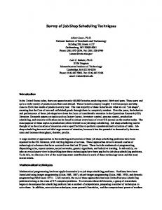
Figure 4. Results as the number of users online increases: Number of serviced users
and since each competing algorithm is capable of actually executing different numbers of jobs, we have used alternative metrics other than makespan and flowtime to compare scheduler performance. Below, the experiments have been performed with the aim of maximizing the trade-off between the number of serviced users by the Cloud –among all users that are connected to the Cloud– and the throughput of jobs that are executed each time a new user connects to the Cloud. The number of executed jobs for each user U in the time i was calculated as NumberJobUi = TotalNumberExecutedJobsi − TotalNumberExecutedJobsi−1 . Irrespective of the metric, in this work we show average results which arises from averaging 10 times the execution of each algorithm. Figures 4, 5 and 6 illustrate the number of serviced users by the Cloud, the number of executed jobs by user and the number of created VMs by each algorithm, respectively. Sub-figures in Figures 4 5 and 6 represent the cases when a constant number of users are joined to Cloud every 60, 90 and 120 seconds. Among all approaches, BE is the algorithm that serves fewer users but executes a number of jobs by user (job rate) greater than Random and ACO. Random serves more users than ACO and BE but with lower job rate. Here, it is important to note that while Random serves as many users may not be fair with the response times for users. The reason behind this is that the Random algorithm assigns randomly the VMs to physical resources, and many of the creations of the VMs requested by users can fail. There are
Users join to the Cloud every 60 seconds 6
Users join to the Cloud every 90 seconds 8
ACO Best Effort Random
7
ACO Best Effort Random
Number of executed jobs (More is better)
Number of executed jobs (More is better)
5
4
3
2
6 5 4 3 2
1 1 0
0 10
20
30
40
50
60
70
80
10
20
30
Number of users online
40
50
60
70
80
Number of users online
Users join to the Cloud every 120 seconds 10
ACO Best Effort Random
Number of executed jobs (More is better)
8
6
4
2
0 10
20
30
40
50
60
70
80
Number of users online
Figure 5. Results as the number of users online increases: Number of executed jobs per user
situations where for a single user Random is able to create only one VM where all jobs of the user are executed. This situation means that the user must wait too long to complete their jobs and thus loses the benefit of running into a Cloud. Finally, ACO performs the best balance with respect to all metrics in question. Table 3 summarizes the position of ACO for each metric with respect BE and Random. ACO algorithm is, on one hand, the algorithm with the best trade-off between the number of serviced users and the number of executed jobs with respect to BE, and on the other hand, ACO offers the best trade-off between the number of executed jobs by user and the number of created VMs with respect to the number of serviced users of Random. These results are encouraging because they indicate that ACO is very close to obtaining the best possible solution but making less use of the network, due to the fact that ACO sends at least 20% fewer network messages than BE, which has an acknowledgeable impact on performance if properly modeled in the simulation. The reason that the schedulers can not serve all users that connect to the Cloud is because the attempt to create VMs fails when the user requests them. The creation of some VMs fails since at the moment a user issues the creation, all physical resources are already fully busy with VMs belonging to other users. Depending on the algorithm and according to the results, some schedulers are able to find to some extent a host with free resources to which at least one VM per user is allocated.
Users join to the Cloud every 60 seconds 120
Users join to the Cloud every 90 seconds
ACO Best Effort Random
140 120 Number of created VMs
100 Number of created VMs
ACO Best Effort Random
80
60
40
100 80 60 40
20
20
0
0 10
20
30
40
50
60
70
80
10
20
30
Number of users online
40
50
60
70
80
Number of users online
Users join to the Cloud every 120 seconds 160
ACO Best Effort Random
Number of created VMs
140 120 100 80 60 40 20 0 10
20
30
40
50
60
70
80
Number of users online
Figure 6. Results as the number of users online increases: Number of created VMs
Serviced Users
Executed Jobs
Created VMs
Random
BE
BE
ACO
ACO
ACO
BE
Random
Random
Table 3. Position of ACO results with respect to BE and Random
Tables 4, 5 and 6 shows the reductions or gains obtained by BE algorithm regarding ACO and Random when a constant number of users join to the Cloud every 60, 90 and 120 seconds, respectively. The gain is calculated considering the number of executed jobs for each group of users u = 10, 20, ..., 80, i.e., %GainUsersu=10,20,30,40,50,60,70,80 = u (ACO&Random)∗100 100 − (numberExecutedJobs . (numberExecutedJobsu (bestE f f ort)) Some observations are that, when 10 users join to the Cloud every 60 seconds the gain of BE with respect to ACO is 6.09% and with respect to Random is 15.22%. This result indicates that ACO is much closer to BE than Random. Moreover, in the worst case – when the number of users is 20 and they are connected to the Cloud every 60 seconds– BE wins to ACO in 12.73% but Random loses in the worst case by 26.57%. The highest gains in terms of number of executed jobs of BE compared to ACO were achieved when users were connected to the Cloud every 90 seconds and reaches 12.80%
Table 4. % Gain of BE regarding ACO and Random. Scheduler
Constant number of users connected each time every 60 seconds 10
20
30
40
50
60
70
80
BE (executed jobs)
4.60
4.95
3.53
3.03
2.76
2.53
2.37
2.23
ACO (executed jobs)
4.32
4.32
3.36
2.99
2.70
2.46
2.07
2.02
Gain BE w.r.t. ACO (0-100%)
6.09
12.73
4.81
1.24
2.03
2.96
12.71
9.27
BE (executed jobs)
4.60
4.95
3.53
3.03
2.76
2.53
2.37
2.23
Random (executed jobs)
3.90
3.64
3.32
2.90
2.68
2.31
2.21
1.87
Gain BE w.r.t. Random (0-100%)
15.22
26.57
5.94
4.30
2.97
9.01
6.99
15.79
Table 5. % Gain of BE regarding ACO and Random. Scheduler
Constant number of users connected each time every 90 seconds 10
20
30
40
50
60
70
80
BE (executed jobs)
6.30
5.90
4.63
4.05
3.60
3.23
2.86
2.63
ACO (executed jobs)
6.05
5.15
4.14
3.88
3.48
2.97
2.90
2.77
Gain BE w.r.t. ACO (0-100%)
3.97
12.80
10.72
4.26
3.33
8.04
-1.40
-5.48
BE (executed jobs)
6.30
5.90
4.63
4.05
3.60
3.23
2.86
2.63
Random (executed jobs)
5.53
4.77
3.89
3.41
3.35
2.92
2.85
2.69
Gain BE w.r.t. Random (0-100%)
12.22
19.15
16.12
15.86
6.89
9.85
0.25
-2.48
Table 6. % Gain of BE regarding ACO and Random. Scheduler
Constant number of users connected each time every 120 seconds 10
20
30
40
50
60
70
80
BE (executed jobs)
7.90
6.95
5.80
4.98
4.36
3.68
3.41
3.21
ACO (executed jobs)
7.72
6.23
5.23
4.48
4.12
3.74
3.46
3.24
Gain BE w.r.t. ACO (0-100%)
2.28
10.36
9.89
10.05
5.55
-1.54
-1.34
-0.86
BE (executed jobs)
7.90
6.95
5.80
4.98
4.36
3.68
3.41
3.21
Random (executed jobs)
7.06
5.59
4.95
4.28
3.77
3.66
3.23
3.15
Gain BE w.r.t Random (0-100%)
10.63
19.57
14.71
14.07
13.62
0.63
5.40
1.95
(when up to 20 users had connected). When users are connected further distanced in time, in our experiments every 120 seconds, the gains percentages of BE decreases. This is sound since adding more users to the environment under test ends up saturating its execution capacity, and thus BE scheduling decisions have less impact on the outcome. This also happens because BE is not an adaptive algorithm like ACO. BE use all available
resources to serve the first users connecting to the Cloud leaving without serving the other. An observation is that in some cases –the cells with negative percentage values in Tables 5 and 6–, ACO wins to BE. These results are very encouraging because it means that ACO, to be an adaptive algorithm, when the number of users increases it achieves a better service to users than BE executing a greater number of jobs. On the other hand, ACO is more fair with the number of users served, and moreover improves when the number of users connected to Cloud every 90 and 120 seconds is larger. In the best case, when users are joined to the Cloud every 120 seconds, the number of serviced users reaches approximately 27. As it has been shown in these experiments, ACO is the algorithm that achieves a better trade-off between the number of serviced users and the executed jobs rate per user. Although that BE is the algorithm that achieves better jobs rate in most tests, small gains were obtained with ACO when users join to the Cloud every 90 and 120 seconds. When joining to the Cloud more users –70 and 80 users– every 90 seconds, the gains were 1.40% and 5.48%, respectively, and when joining to the Cloud 60, 70 and 80 users every 120 seconds, the gains were 1.54%, 1.34% and 0.86%, respectively.
5. Related work The last decade has witnessed an astonishingly amount of research in improving SI techniques, specially ACO [20]. As shown in recent surveys [24,21], these techniques have been applied to distributed job scheduling. However, with regard to scheduling in Cloud environments, very few works can be found to date [17], and moreover, to the best of our knowledge, no effort aimed to job scheduling based on SI for dynamic scientific Clouds where a large number of users are connected to submit their experiments. In this related works, it is important to note that, on one hand, the SI techniques are used to solve the job scheduling problem, i.e., solve how the jobs are assigned to VMs, and do not to solve VM scheduling problem. On the other hand, the objectives to optimize considered by the authors are suitable when the execution of a set of jobs belong to the same user, but when a large number of users make requests to the Cloud another metrics and goals such as those proposed in this work should be considered. Concretely, the works in [1,25] propose ACO-based Cloud schedulers for minimizing makespan and maximizing load balancing, respectively. An interesting aspect of [1] is that it was evaluated using real Cloud platforms (Google App Engine and Microsoft Live Mesh), whereas the other work was evaluated through simulations. However, during the experiments, [1] used only 25 jobs and a Cloud comprising 5 machines, while in [25] despite to be simulated the authors have not provided all the information needed to reproduce their experiments. Interestingly, like our proposal, these two efforts support dynamic resource allocation, i.e., the scheduler does not need to know the details of the jobs to allocate and the available resources. Another relevant approach based on Particle Swarm Optimization (PSO) is proposed in [19]. PSO is another SI technique that mimics the behavior of bird flocks, bee swarms and fish schools. Contrary to [1,25] and our scheduler, the approach is based on static resource allocation, which forces users to feed the scheduler with the estimated running times of jobs on the set of Cloud resources to be used. Besides, [19] is targeted at paid Clouds, i.e. those that charge users for CPU, storage and network usage. As a consequence, the work only minimizes monetary cost, and does not consider other metrics.
Finally, the work in [12] address the problem of job scheduling in Clouds while reducing energy consumption. Indeed, energy consumption has become a crucial problem [13], on one hand because it has started to limit further performance growth due to expensive electricity bills, and on the other hand, by the environmental impact in terms of carbon dioxide (CO2) emissions caused by high energy consumption. This in fact has gave birth to a new field called Green Computing [13]. As such, [12] pays attention to achieve competitive makespan as evidenced by experiments performed via CloudSim [4], which is also used in this paper. It is worth noting that all the surveyed works ignore multiple users, rendering difficult their applicability to execute PSEs in dynamic scientific Cloud environments.
6. Conclusions PSEs is a type of simulation that involves running a large number of independent jobs and typically requires a lot of computing power. These jobs must be efficiently processed in the different computing resources of a parallel environment such as the ones offered by a Cloud. Then, job scheduling in this context plays a fundamental role. Recently, SI-inspired algorithms have received increasing attention in the research community. SI refers to the collective behavior that emerges from a swarm of social insects. Social insect colonies collectively solve complex problems by intelligent methods. These problems are beyond the capabilities of each individual insect, and the cooperation among them is self-organized without any supervision. Through studying social insect colonies behaviors such as ant colonies, researchers have proposed algorithms for combinatorial optimization problems. Moreover, job scheduling in Clouds is also a combinatorial optimization problem, and some SI-inspired schedulers have been proposed. Existing efforts do not address dynamic online environments where multiple users connect to scientific Clouds to execute their PSEs and to the best of our knowledge, no effort aimed at maximizing the number of serviced users in a Cloud and maximizing the number of executed jobs for each user that is joined. Executing a greater number of jobs every time a user is connected means a more agile human processing of PSE job results. Therefore, our new two-level Cloud scheduler pays special attention to this aspect and the total number of user serviced. Simulated experiments performed with the help of the well-established CloudSim toolkit and real PSE job data show that our scheduler can balance better than their competitors the trade-off between the number of serviced users and the job execution rate by user. Moreover, the ACO algorithm is the closest to Best effort with respect to job rate and there are situations where higher gains are achieved by ACO when there are a large number of users connected every 90 to 120 seconds. We believe these are quite encouraging results. Eventually, we will materialize the resulting schedulers on top of a real Cloud platform, such as Emotive Cloud (http://www.emotivecloud.net/) or OpenNebula (http://opennebula.org/), which are designed for extensibility. Lastly, we will consider other Cloud scenarios, for example, with heterogeneous machines. Another issue concerns energy consumption by the scheduler itself. Simpler schedulers (e.g. Random or “Best effort”) require less CPU usage, memory accesses and network transfers compared to more complex policies such as our scheduler. For example, we need to maintain host load information for ants, which requires those resources.
Therefore, when running many jobs, the accumulated resource usage overhead may be arguably significant, resulting in higher demands for energy. Finally, we are extending this work by incorporating a mechanism that, every certain time intervals, retries the creation of all or some of the VMs that failed when the user requested them. Preliminary results show that, compared to the results reported in this paper, our ACO-based scheduler is still the most competitive regarding jobs rate and at the same time improvements the number of serviced users.
Acknowledgements We acknowledge the financial support provided by ANPCyT through grants PAE-PICT 2007-02311, PAE-PICT 2007-02312 and National University of Cuyo project 06/B194. The third author acknowledges her Ph.D. fellowship granted by PRH-UNCuyo Project.
References [1] [2] [3]
[4]
[5]
[6] [7] [8] [9]
[10]
[11]
[12]
[13]
S. Banerjee, I. Mukherjee, and P. Mahanti. Cloud Computing initiative using modified ant colony framework. In World Academy of Science, Engineering and Technology, pages 221–224. WASET, 2009. E. Bonabeau, M. Dorigo, and G. Theraulaz. Swarm Intelligence: From Natural to Artificial Systems. Oxford University Press, 1999. R. Buyya, C. Yeo, S. Venugopal, J. Broberg, and I. Brandic. Cloud computing and emerging IT platforms: Vision, hype, and reality for delivering computing as the 5th utility. Future Generation Computer Systems, 25(6):599–616, 2009. R. Calheiros, R. Ranjan, A. Beloglazov, C. De Rose, and R. Buyya. CloudSim: A toolkit for modeling and simulation of Cloud Computing environments and evaluation of resource provisioning algorithms. Software: Practice & Experience, 41(1):23–50, 2011. C. Careglio, D. Monge, E. Pacini, C. Mateos, A. Mirasso, and C. García Garino. Sensibilidad de resultados del ensayo de tracción simple frente a diferentes tamaños y tipos de imperfecciones. In M. G. E. Dvorkin and M. Storti, editors, Proceedings of II South American Congress on Computational Mechanics (MECOM 2010), Mecánica Computacional, volume XXIX, pages 4181–4197, Buenos Aires, Argentina, 2010. AMCA. ISSN 1666-6070. T. L. Casavant and J. G. Kuhl. A taxonomy of scheduling in general-purpose distributed computing systems. IEEE Transactions on Software Engineering, 14(2):141–154, Feb. 1988. M. Dorigo. Optimization, Learning and Natural Algorithms. Phdthesis, Politecnico di Milano, Italy, Milano, Italy, 1992. C. García Garino, F. Gabaldón, and J. M. Goicolea. Finite element simulation of the simple tension test in metals. Finite Elements in Analysis and Design, 42(13):1187–1197, 2006. C. García Garino, C. Mateos, and E. Pacini. Job scheduling of parametric computational mechanics studies on cloud computing infrastructures. International Advanced Research Workshop on High Performance Computing, Grid and Clouds. Cetraro (Italy), June 2012. C. García Garino, M. Ribero Vairo, S. Andía Fagés, A. Mirasso, and J.-P. Ponthot. Numerical simulation of finite strain viscoplastic problems. Journal of Computational and Applied Mathematics, (0), 2012. doi:10.1016/jcam.2012.10.008. ISSN: 0377-0427. In press. W. Huang, J. Liu, B. Abali, and D. Panda. A case for high performance computing with virtual machines. ´ pages 125–134, In Proceedings of the 20th annual international conference on Supercomputing, ICS 06, New York, NY, USA, 2006. ACM. ISBN: 1-59593-282-8. R. Jeyarani, N. Nagaveni, and R. Vasanth Ram. Design and implementation of adaptive power-aware virtual machine provisioner (APA-VMP) using swarm intelligence. Future Generation Computer Systems, 28(5):811–821, 2012. Y. Liu and H. Zhu. A survey of the research on power management techniques for high-performance systems. Software Practice & Experience, 40(11):943–964, October 2010.
[14] [15] [16]
[17]
[18]
[19]
[20] [21] [22]
[23]
[24] [25]
S. Ludwig and A. Moallem. Swarm intelligence approaches for grid load balancing. Journal of Grid Computing, 9(3):279–301, 2011. C. Mateos, A. Zunino, and M. Campo. On the evaluation of gridification effort and runtime aspects of jgrim applications. Future Generation Computer Systems, 26(6):797 – 819, 2010. C. Mateos, A. Zunino, M. Campo, and R. Trachsel. BYG: An Approach to Just-in-Time Gridification of Conventional Java Applications. In F. Xhafa, editor, Parallel Programming, Models and Applications in Grid and P2P Systems, volume 17, pages 232–260. IOS Press, 2009. ISBN: 978-1-60750-004-9. E. Pacini, C. Mateos, and C. García Garino. Schedulers based on ant colony optimization for parameter sweep experiments in distributed environments. In Dr. Siddhartha Bhattacharyya, Dr. Paramartha Dutta, editor, Handbook of Research on Computational Intelligence for Engineering, Science and Business, volume I, chapter 16, pages 410–447. IGI Global, 2012. ISBN13: 9781466625181. E. Pacini, M. Ribero, C. Mateos, A. Mirasso, and C. García Garino. Simulation on cloud computing infrastructures of parametric studies of nonlinear solids problems. In F.V. Cipolla-Ficarra et al., editor, Advances in New Technologies, Interactive Interfaces and Communicability (ADNTIIC 2011), volume 7547 of LNCS, pages 56–68. Springer-Verlag, 2011. ISBN 978-3-642-34009-3. S. Pandey, L. Wu, S. Guru, and R. Buyya. A particle swarm optimization-based heuristic for scheduling workflow applications in Cloud Computing environments. In International Conference on Advanced Information Networking and Applications, pages 400–407. IEEE Computer Society, 2010. M. Pedemonte, S. Nesmachnow, and H. Cancela. A survey on parallel ant colony optimization. Applied Soft Computing, 11(8):5181–5197, 2011. M. Tinghuai, Y. Qiaoqiao, L. Wenjie, G. Donghai, and L. Sungyoung. Grid task scheduling: Algorithm review. IETE Technical Review, 28(2):158–167, 2011. L. Wang, J. Tao, M. Kunze, A. C. Castellanos, D. Kramer, and W. Karl. Scientific cloud computing: Early definition and experience. In 10th IEEE International Conference on High Performance Computing and Communications, pages 825–830, Washington, DC, USA, 2008. IEEE Computer Society. G. Woeginger. Exact Algorithms for NP-Hard Problems: A Survey. In M. Junger, G. Reinelt, and G. Rinaldi, editors, Combinatorial Optimization - Eureka, You Shrink!, volume 2570 of Lecture Notes in Computer Science, pages 185–207. Springer Berlin/Heidelberg, 2003. F. Xhafa and A. Abraham. Computational models and heuristic methods for Grid scheduling problems. Future Generation Computer Systems, 26(4):608–621, 2010. Z. Zehua and Z. Xuejie. A load balancing mechanism based on ant colony and complex network theory in open Cloud Computing federation. In 2nd International Conference on Industrial Mechatronics and Automation, pages 240–243. IEEE Computer Socienty, 2010.
About the authors Carlos García Garino (http://itic.uncu.edu.ar/lapic/members/) received the Ph.D. degree from Universidad Politécnica de Cataluña, Barcelona, España, in 1993, and the Civil Engineering degree from Universidad Nacional de Buenos Aires, Argentina, in 1978. Currently he is Professor of Facultad de Ingeniería at UNCuyo, and director of Instituto Universitario para las Tecnologías de la Información y las Comunicaciones (ITIC), UNCuyo. His current research interests are Computer Networks, Distributed Computing and Computational Mechanics. Cristian Mateos (http://www.exa.unicen.edu.ar/~cmateos) received a Ph.D. degree in Computer Science from the UNICEN, in 2008, and his M.Sc. in Systems Engineering in 2005. He is a full time Teacher Assistant at the UNICEN and member of the ISISTAN and the CONICET. He is interested in parallel/distributed programming, Grid middlewares and Service-oriented Computing. Elina Pacini received a BSc. in Information Systems Engineering from the UTN-FRM in 2005. She is working on his Ph.D. thesis since 2010 under the supervision of Carlos García Garino and Cristian Mateos. Her thesis topic is Cloud scheduling for parameter sweep experiments based on Swarm Intelligence techniques.