rectangular objects, which are, in office- and museum-like environments, the .... based on projective geometry and the corner points of the rectangular object can ...
Acquiring Models of Rectangular 3D Objects for Robot Maps Derik Schr¨oter and Michael Beetz Technische Universit¨at M¨unchen Boltzmannstr. 3, 85748 Garching b. M¨unchen, Germany schroetdin.tum.de, beetzin.tum.de http://www9.in.tum.de/people/schroetd/Research/ Abstract— State-of-the-art robot mapping approaches are capable of acquiring impressively accurate 2D and 3D models of their environments. To the best of our knowledge few of them can acquire models of task-relevant objects. In this paper, we introduce a novel method for acquiring models of taskrelevant objects from stereo images. The proposed algorithm applies methods from projective geometry and works for rectangular objects, which are, in office- and museum-like environments, the most commonly found subclass of geometric objects. The method is shown to work accurately and for a wide range of viewing angles and distances.
I. I NTRODUCTION Many autonomous mobile service robots use maps, models of their environments, as resources to perform their tasks more reliably and efficiently. A number of software systems and algorithms for the autonomous acquisition of environment maps of office buildings, museums, and other indoor environments have been developed [2], [7], [11], see [12] for an extended overview of state-of-the-art mapping approaches. While most recent mapping algorithms have been designed to acquire very accurate maps [5], [10], [6], little attention has been paid to extend these algorithms to acquire additional information about their environments. Information that makes environment maps more informative for service robot applications include representations of the environment structure, object hypotheses, and characteristics of substructures that affect navigation and exploration. Vision-based aquisition of 3D environment maps has been pioneered by Ayache and Faugeras [1] who built and updated three-dimensional representations based on vision sensors. Kak and his colleagues used semi-automatically acquired 3D models of hallway environments for visionbased navigation, in [4] he gives a recent and comprehensive survey of the respective research area. In this paper we extend an existing robot mapping framework, namely RG mapping (range data based Region and Gateway mapping) [3], by means for automatically acquiring models of rectangular 3D objects. In many indoor environments such as office buildings or museums rectangular objects play key roles. Their importance is depicted in figure 1. Also, many other objects, such as pieces of furniture are composed of rectangular objects. The proposed method for the acquisition of models for rectangular works as follows. The robot explores its operating environment in order to acquire an RG map. During the exploration phase it captures stereo images and
Fig. 1. Rectangular objects in typical office environments. The upper two images show that in office environments many of the task-relevant objects are rectangular or cubic. The lower two images give an illustrative view of the visual recognition of rectangular objects in an image and how rectangular objects are stored in maps.
uses the stereo images to recognize rectangular objects and estimate their 3D position and orientation with respect to its RG map. The 3D models of the objects are then stored in the RG map. Our method advances the state of the art in object acquisition and map building in the following ways. It uses methods from stereo image processing and projective geometry to detect rectangular objects and acquire 3D models for them. Rectangular and cubic objects, which are composed of rectangles, are probably the single most important object classes in many indoor environments, such as office buildings and museums. The method is shown to be impressively accurate and shown to work for a wide range of distances and viewing angles. The remainder of the paper is organized as follows. Section II describes RG mapping, the mapping framework that our object model acquisition method is embedded in. We will then describe the necessary formulas from projective geometry, in particular the method for estimating the plane normal of the rectangle. We conclude with our experimental results, a discussion, and an outline of our next research steps.
region 08
region 06
region 05
region 10
region 02
region 01
The arrows mark identical gateways. Thereby, if the two involved regions are represented within the same coordinate system (CS) the gateway points are numerically identical. Otherwise a CS transformation has to be applied on traversal. region 09
Fig. 2.
region 07
region 04
region 03
RG map of our department floor at TUM IX (Orleanstreet, Munich). Raw data: 761 laser scans, ca. 65000 points.
II. RG M APPING We develop our mechanisms for the acquisition of object models in the context of RG mapping [3]. RG mapping aims at the autonomous acquisition of structured models of indoor environments, in particular office and museum-like environments, where the models contain explicit representations of task-relevant objects. RG maps represent environments as a set of regions connected by gateways. Regions are described compactly using a set of line segments and classified into different categories such as “office-like” or “hallway-like” regions. Regions contain models of objects within the regions, a class label, a compact geometric description, a bounding box, one or two main axes and a list of adjacent gateways, and provide additional information including measures of accuracy and completeness. The gateways represent transitions between regions. In indoor environments several types of gateways can be distinguished, e.g. hallway T/L/X-junctions as well as small passages and changes from a rather narrow hallway into an open room, e.g. a lobby. Gateways are specified by a class label, adjacent regions, traversal directions, crossing-points and gateway-points that can be used for detecting when a gateway is entered and left. Figure 2 shows how an office environment is represented as an RG map. It comprises nine regions, which are connected by gateways of type narrow passage. The regions are visualized through their geometric description, the set of line segments. Among other things, the geometric 2D description is used to predict the laser scan that the robot should receive at a given location within the region. Note that the geometric description contains lines that are outside the region’s bounding box. This is because these lines can be seen through the gateway and used for robot self-localization.
The final components of the maps are the object hypotheses. In the reminder of this paper we show that representations of arbitrary rectangular 3D objects can be automatically acquired. Thereby the 3D position, height and width of the objects are not known in advance.
Hardware - Stereo Camera Head - Laser Range Finder - Drive + Odometry - and others
Gateway Detection
Scan Mapper Scan Matching from Gutmann & Konolige
Stereometry Small Vision System from SRI
Fig. 3.
Reconstruction of 3D Objects e.g. rectangular, cuboid
Region & Gateway Mapping
3D Object reconstruction within the RG Mapping framework
Figure 3 depicts the integration of the reconstruction and stereo modules into the RG mapping system [3]. For clarity reasons, the figure focuses on the vision part and the interaction of those modules with the other RG mapping components. The overall RG mapping and control system also involves modules for collision avoidance, localization and path planning. Also the module denoted as hardware consists of several independent modules for data acquisition (laser, camera, sonar, odometry) as well as synchronization of data and odometry sources and low level drive control. The stereometry module receives two images and calculates the disparity and depth map [9]. For the reconstruction of 3D objects presented in section III one rectified image and the depth map must be provided by the hardware and the stereo module, respectively. The scan mapper module aligns consecutive scans according to the scan matching
algorithms described in [5]. And the gateway detection continuously analyzes laser scans to detect when gateways are present and when they have been passed. The RG mapping module collects this information together with the aligned scans and the reconstructed 3D objects in order to: • structure the 2D information into regions and gateways, • extract a compact 2D description for the regions from the laser range data (set of line segments, bounding box, 2D object hypotheses, main axes etc.), • add the 3D information from the reconstruction module to the 2D description. In the following section we outline how models of rectangular 3D objects can be acquired from image data. III. ACQUIRING MODELS OF RECTANGULAR OBJECTS The acquisition of object models is performed as follows. First, object hypotheses, i.e. quadrangles in R2 , that may be projections of rectangular objects in R3 , are extracted from a single image. Then, the plane normal nP is calculated based on projective geometry and the corner points of the rectangular object can be reconstructed in R3 by ray-planeintersection. This yields the description of the object in the camera coordinate system (CCS). Finally, region-based (or global) registration, e.g. scan matching based on laser range data [5], is applied to transform those object representations into a region based (or global) coordinate frame. In the ideal case the presented algorithm provides perfect reconstruction. In this case ”ideal” means, that no spatial discretization by the sensor and exact depth measurements for single points are assumed. Both is obviously not the case in a real world application, but practical experiments have shown that the approach is robust against such error sources (discretization or quantization, erroneous measurements). Furthermore, false hypotheses are automatically rejected in the step of ray-plane intersection. A. Generating object hypotheses in the image plane Pixels in the image that represent edges are detected by an edge filter, e.g. Sobel, Canny, Deriche etc. The pixels are then concatenated to line segments, and merged together if they lie on the same line and their endpoints are close to each other. Small single line segments are rejected. Based on this set of M line segments, hypotheses are generated by grouping. With grouping we mean to generate N sets of four-line tuple out of all M segmented lines (M>N). The simplest way of forming those four-line tuples is to consider all possible combinations and reject hypotheses, which are not plausible. The following configurations cannot result from a projected 3D rectangle: • 3 or 4 almost parallel lines, • opposite lines with direct intersection, • very large (respectively very small) internal angles (This issue will be discussed in section IV.) These constraints are exploited in the grouping process and reduce the number of explicitly generated four-line tuples. The resulting set of four-line tuples contains our candidates for projections of rectangular 3D objects. Therefore they are processed further.
B. Estimating the plane normal Assuming a rectangular object, which lies in the plane Π, we estimate the plane normal nΠ by the means of projective geometry. In the projective space P n , points P P and lines LP are specified in homogeneous coordinates (of dimension n + 1), in particular for P P , LP � P 2 : P P P P P P P P = (pP 1 , p2 , p3 ) and L = (lP1 , lP 2 , l3 ) p1 p2 R 2 where P � R = (x, y) = ( pP , pP ) 3 3 The cross product of two points in P 2 defines the line in P 2 , which connects those two points. And similarly, the cross product of two lines in P 2 defines the intersection point of those two lines in P 2 . Considering two lines which are parallel in R3 with their projection on the image plane P P P beeing LP 1 and L2 . The intersection of L1 and L2 is called vanishing point PvP . P PvP = LP 1 × L2
(1) 3
Taking all possible sets of parallel lines in R , which lie in the same plane (including rotation, translation and scaling within the plane), results in a set of vanishing points in P 2 , which lie all on the same line in P 2 . This is the vanishing 3 line LP v . Actually, for each plane in R , there exists exactly 2 one vanishing line in P , and the corresponding relationship can be utilized to calculate the plane normal in R3 (see eq. 2). For further detail about projective geometry and the point-line-dualism in P 2 refer to the very well written book by Hartley and Zissermann [8]. Given a calibrated camera with camera matrix C, the plane normal np in R3 is calculated from the vanishing line by: (2) n P = C T · LP v The camera parameters are determined in advance by calibration procedures. Hence, radial distortion can be removed from the images. We assume the principal point (Cx , Cy ) to lie in the center of the camera coordinate system (CCS). That means, it is necessary, to perform a translation by (Cx , Cy ) on the point features extracted from the image, prior to calculating the plane normal. The following camera matrix C results from those considerations and is used to determine the plane normal: f 0.0 0.0 sx C = 0.0 sf 0.0 y 0.0 0.0 1.0 Where f denotes the focal length and (sx , sy ) refer to width and height of a pixel, respectively. Note that (Cx , Cy ) must also be known. The algorithm can be summarized as follows: 1) Transforming the given lines from R2 to P 2 . A line LR is described by two points (P1R , P2R ). We transform the single points from R2 into P 2 and determine the line in P 2 with the cross product: P P = (p1 , p2 , p3 ) = (x − Cx , y − Cy , 1.0) P P LP v = P1 × P2 P P 2) Calculate P1v , P2v for the two sets of opposite lines with eq. 1. P P 3) Calculate the vanishing line LP v = P1v × P2v 4) Calculate the plane normal with eq. 2
C. Ray-Plane Intersection Considering a pinhole camera model, all rays intersect in the camera center P C , which has been chosen to be the origin of the CCS. The original Point P in R3 and the projected point P’ both lie on this line and obviously the following relation ship holds: P CP = P C + λ · P CP 0 → P = λ · P0
(3)
On the other hand, a vector v1 can be constructed, which is orthogonal to nP , i.e.: n P · v 1 = n x · v 1x + n y · v 1y + n z · v 1z = 0 And from there, vector v2 can be determined according to: v2 = n P × v 1 Given one corner point Picr of the rectangular object in R3 we can derive a plane equation P = Picr + µ1 · v1 + µ2 · v2
i � (1...4)
(4)
All other 3D points can then be calculated by ray-plane intersection, i.e. solving the system of linear equations (3,4) for the corner point in R3 . Note the points Pi0 (i = 1..4) � R2 from the image must first be transformed into the CCS. Thereby, the z-coordinate is the focal length. It is also possible to set an arbitrary distance and determine a 3D point by the means of eq. 3. If the given 2D quadrangle is in fact a projection of a 3D rectangle, the reconstruction is correct up to a scale factor. That means, in general it is possible to verify or reject the hypothesis without any depth measurements. D. Discussion The presented reconstruction algorithm is exact, if we neglect discretization in the image sensor and inaccuracies of depth measurements. That means, given a projected 3D rectangle, i.e. a quadrangle in 2D, the plane normal can be calculated accurately. Given the ray-plane intersection, the 3D rectangle can be determined up to scaling and translation along the optical axis. Both parameters are directly correlated. Adding the 3D coordinates of one corner point, defines the rectangular object uniquely. IV. E XPERIMENTAL R ESULTS In this section, we will empirically evaluate the accuracy and robustness of the model acquisition of rectangular objects from stereo. We have stated in the discussion paragraph of the last section that for non-discrete sensors with accurate 3D measurements our method is accurate. In this section we will vary the discretization resolution and apply the reconstruction method to images captured by our B21 robot in order to evaluate the method under realistic conditions and in real settings. To do so, we will first evaluate the influence of pixel discretization on reconstruction robustness and accuracy based on simulation (section IV-A). The use of simulation enables us to make more controlled experiments, in which we can vary the discretization resolution of non-discrete image sensors (which cannot be done with the real imaging
devices) and access ground truth data easily. We will then assess the impact of inaccuracies in 3D measurements based on results that are obtained in experiments with our B21 robot (IV-B). A. Influence of spatial discretization by the image sensor The experimental setting for assessing the impact of discretization in the image sensor on the reconstruction results is the following. We first generate a virtual image sensor for the user specified resolution of the image sensor discretization. We then systematically generate sets of rectangular objects in 3D space, project them into 2D space in order to produce the input data for our virtual sensor. Our 3D reconstruction method is then applied to the output of the virtual sensor and then compared to the real 3D position of the rectangular object. We classify the outcome into three categories: first, the reconstruction failed; second, the reconstruction succeeded but was inaccurate; and third, the reconstruction was accurate.
Fig. 4. Reconstructable (left) and non-reconstructable (right) projections due to spatial discretization in the image sensor
To give you an intuition about which 3D poses can be accurately reconstructed and which ones not, we have visualized both sets in figure 4. In this particular experiment, we have placed a 3D rectangle at z = 1 meter and the camera at z = - 3 meter. Then the rectangle was rotated stepwise in 3D by 36 degree around the z-, x- and y-axis, which gives us a total of 1000 3D poses of the object. The parameters of the virtual camera are set to 766×580 pixels resolution, sx≈sy= 8.3 · 10−3 meter, Cx =391.685, Cy =294.079 and focal length of 0.00369 meter, which are the estimated parameters of the cameras on the robot. The accuracy is defined as the length of the error vector between the reconstructed and the original 3D point. Our results show, that despite the inaccuracies caused by discretization, the algorithm still gives very good result. From some projections reconstruction is not possible. But those cases can clearly be classified, as can be seen later. Figure 4 (left) shows the set of projections, that can accurately be reconstructed. These are 968 of the 1000 poses that are reconstructed with an error of less than 10 centimeters. In the majority of cases the error is substantially smaller. Figure 4 (right) shows the 32 projections which cannot be reconstructed. You can see that these 2D quadrangles are characterized by very large (more than 150 degree) and very small internal angles. We have also performed
this experiment with smaller angle step sizes in order not to miss any other special cases. But there are none. In fact, the percentage of non-reconstructable projections is always about eight percent of the whole considered set. And this is due to the before mentioned special cases of quadrangles. Furthermore, we found that projections with bad reconstruction results are close to the configuration where the reconstruction failed. To get additional evidence for these findings, we have learned rules for predicting whether or not a reconstruction of a rectangular object will be accurate or at least possible. We have trained the decision tree with the angles of 64000 projected objects and whether or not the reconstruction has been successful. The angle α for each of these projections P4 was determined as follows: α = i=1 |αi − π| Where αi denote the internal angles of the quadrangle in R2 . That means we take the deviation of the internal angles to 90 degree as criterion, because we assume from the experiments above, that reconstruction problems result from very large and very small internal angles. The learning algorithm came up with compact rules that predict when the reconstruction will fail and when it will succeed. As a result, two rules have been learned: Rule 1: sum_angle class true [98.2%] (53796 used samples) Rule 3: sum_angle > 314.908 -> class false [79.2%] (3992 used samples)
For interpretation purposes we also consider the average deviation: αmean = α4 Rule 1 says that if α is smaller than 284 degrees the prediction will succeed. This rule has captured more than 80% of the cases and a prediction accuracy of 98%. That means, we have a high probability, that the reconstruction will succeed for αmean < 71 degree, hence for 19 degree < αi < 161 degree. The second rule that predicts failure applies if α is larger than 314 degree with an expected prediction accuracy of about 80%. With the same rational, we can conclude, that αi > 168 degree and αi < 12 degree causes critical cases. We conducted the same experiment for projections with good and bad reconstruction results, where bad refers to errors larger then 5 centimeter. Thereby the cases where the reconstruction would fail have been neglected. In this case, more than two rules have been learned, but the summarized conclusions are the same. In a certain range of angle αi , we have a high probability, that the reconstruction error is smaller than 5 centimeter, and outside of this range the error increases. That means, by limiting the internal angles for the quadrangle hypotheses to be considered, we can not only guarantee with high probability, that the reconstruction will succeed, but also that the error does not exceed a certain upper bound. We conclude from these experiments that the presented algorithm can robustly deal with effects of pixel discretization, and rectangles can be very accurately reconstructed as long as the internal angles of the projection, i.e. the 2D-quadrangle, lie in a certain range around 90 de-
gree (26 < αi < 154). a) Discussion: Even more important than the apparent robustness and accuracy of the reconstruction method is that we can build predictive models for the accuracy and success of applying the method to a given group of lines. This is because the reconstruction step is a step of an autonomous exploration process that the robot performs to acquire a map of its environment. Thus, if the robot detects that a particular reconstruction is not promising it can infer a position from which the reconstruction of the hypothesized object is likely to succeed. B. Influence of inaccurate 3D-measurements We have studied the influence of errors in depth measurements with real world image data. Depth measurements have been generated with the Small Vision System from SRI [9]. As stated above inaccuracies from 3D measurements can be evaluated by the means of scaling errors. Therefore, we have chosen the width and height of the rectangular object as a criterion for quality measures. In all figures (left) the depicted quadrangles (white) are backward projections of the reconstructed 3D rectangles into the image. It can be seen that these back projections fit very well to the image data. The question is, how well does the reconstructed rectangle describe the actual rectangular object.
Fig. 5.
Door frame experiment 1
Very prominent rectangular objects in a variety of indoor environments are door frames. All door frames depicted here (fig. 5, fig. 6) are 210 centimeter high and 101 centimeter wide. Smaller 3D rectangles include for example posters or white boards (fig. 8) as well as computer monitors (fig. 7) in office environments. The noisy depth measurements are depicted on the right in all those figures. Table I summarizes the reconstruction results for the presented examples. It can be seen that the reconstruction for different scenarios and rectangular objects is very accurate. Which leads to the conclusion that the presented approach is very well suited for automatic generation of representations for 3D rectangular objects in indoor environments. The accuracy increases if more than one 3D corner point can be measured and is given to the reconstruction algorithm. Additionally, the results can be verified by projecting the reconstructed rectangle into the image of the second camera. Thereby, the observations (line segments) of that
Fig. 6.
Door frame experiment 2 experiment Door 1 Door 2, LeftFront Door 2, RightFront Door 2, RightBack White board Monitor
original size 210x101 210x101 210x101 210x101 21.4x30.2 27.0x33.8
reconstructed size 207.2x104.3 208.5x105.3 207.9x105.6 192.0x107.8 21.1x30.9 27.5x34.04
TABLE I S UMMARY OF RECONSTRUCTION RESULTS .
The values for original and reconstructed size denote height×width in centimeters.
camera are compared with the projected (reconstructed) 3D rectangle. Also it can be expected, that tracking those 3D object hypotheses over time and merging the corresponding observation will lead to a further increasing of robustness and accuracy.
Fig. 7.
Monitor in office environment
Fig. 8.
White board in a hallway
V. C ONCLUSIONS We presented a novel approach for acquiring models of task-relevant objects. The reconstruction algorithm developed in this paper is robust against discretization in the image sensor and errors from the depth measurements. That
means rectangular 3D objects can robustly and with high accuracy be reconstructed from their 2D projections and one 3D measurement of a corner point of that object. This has been demonstrated by simulation-based and real world experiments on a B21r mobile robot. The main advantages of this approach can be summarized as follows. Objects are explicitly modeled in the environment map without assuming too much model knowledge. The respective object representations can be autonomously acquired with high accuracy. And information from the subsequent steps of the reconstruction algorithm can be utilized to actively control the exploration behavior. Our ongoing research comprises the following threads of development and investigation. We are currently developing a vision- and laser-based robot navigation system that allows our robot to safely explore indoor environments. This navigation system enables us to fully integrate the vision-based object recognition into our Region & Gateway mapping system and to acquire complete maps with object models. Another line of research investigates and develops object recognition algorithms for other categories of objects, in particular cubic objects like tables, closets etc. The accuracy and robustness of the different reconstruction methods will further be improved by methods, which were discussed in subsection III-A and IV-B. R EFERENCES [1] Nicholas Ayache and Olivier Faugeras. Maintaining Representations of the Environment of a Mobile Robot. Int. Journal of Robotics and Automation, 5(6):804–819, 1989. [2] W. Burgard, A.B. Cremers, D. Fox, D. H¨ ahnel, G. Lakemeyer, D. Schulz, W. Steiner, and S. Thrun. Experiences with an interactive museum tour-guide robot. Artificial Intelligence, 114(1-2), 2000. [3] J.-S. Gutmann D. Schr¨ oter, M. Beetz. Rg mapping: Learning compact and structured 2d line maps of indoor environments. In in Proc. to 11th IEEE ROMAN 2002, Berlin/Germany. [4] Kak A.C. DeSouza G.N. Vision for mobile robot navigation. In in IEEE Transactions on Pattern Analysis and Machine Intelligence, volume 24, Feb. 2002. [5] J.-S. Gutmann and K. Konolige. Incremental mapping of large cyclic environments. In Proc. of the IEEE International Symposium on Computational Intelligence in Robotics and Automation (CIRA), 2000. [6] D. Haehnel, W. Burgard, and S. Thrun. Learning Compact 3D Models of Indoor and Outdoor Environments with a Mobile Robot. In The fourth European workshop on advanced mobile robots (EUROBOT), 2001. [7] D. Haehnel, D. Fox, W. Burgard, and S. Thrun. A highly efficient FastSLAM algorithm for generating cyclic maps of large-scale environments from raw laser range measurements. In In Proc. of the Conference on Intelligent Robots and Systems (IROS), 2003. [8] R. I. Hartley and A. Zisserman. Multiple View Geometry in Computer Vision. Cambridge University Press, ISBN: 0521623049, 2000. [9] K. Konolige. Small vision systems: Hardware and implementation. In in Proc. to 8th International Symposium on Robotics Research, Hayama, Japan, October 1997. [10] Y. Liu, R. Emery, D. Chakrabarti, W. Burgard, and S. Thrun. Using EM to learn 3D models with mobile robots. In Proc. of the International Conference on Machine Learning (ICML), 2001. [11] M. Montemerlo, S. Thrun, D. Koller, and B. Wegbreit. FastSLAM: A factored solution to the simultaneous localization and mapping problem. In Proceedings of the AAAI National Conference on Artificial Intelligence, Edmonton, Canada, 2002. AAAI. [12] S. Thrun. Robotic mapping: A survey. In G. Lakemeyer and B. Nebel, editors, Exploring Artificial Intelligence in the New Millenium. Morgan Kaufmann, 2002.