algorithm which gives the approximate medial axis of a domain bounded by simple, closed ... We report the results of our algorithm for tangent con- tinuous cubic .... the traced branches of the medial axis do not interesect each other, thus making our results ... For example if f : R â R is the square function f(x) = x · x, then a.
ACS Algorithms for Complex Shapes with Certified Numerics and Topology
Prototype implementation of certified approximation of the Medial Axis of smooth curves
Sunayana Ghosh
Gert Vegter
ACS Technical Report No.: ACS-TR-36-26-02 Part of deliverable: WP-II/D6 Site: RUG Month: 36
Project co-funded by the European Commission within FP6 (2002–2006) under contract nr. IST-006413
Abstract In this report we give an algorithm to construct an approximate medial axis of a connected domain without any holes, in 2-D, also known as the simply connected domain. The first part of the report concentrates on the algorithm which gives the approximate medial axis of a domain bounded by simple, closed C 3 curve. In the second part of the report we look at a modified version of which looks at domain bounded by splines, which are piecewise C 3 . We report the results of our algorithm for tangent continuous cubic splines which do not have any extremums of the Euclidean curvature at the point of tangency of two splines. Our algorithm uses interval arithmetic to compute the leaf and the branch points. Using simple combinatorial properties of the Medial Axis we guarantee topological correctness of the output.
1
Introduction
In computer vision and pattern recognition the Medial Axis of a curve is an important shape descriptor of the region enclosed by the curve. The Medial Axis is the closure of the set of centers of maximal free disks enclosed in the curve. In other words, a point is on the Medial Axis if its distance to the curve is attained in at least two points on the curve. Although several algorithms exist for the computation of an approximate Medial Axis, to the best of our knowledge none of these methods guarantees correct topology of the output. We present such a method with topological guarantees for sufficiently smooth (C 3 ) connected curves in the plane. Furthermore, we extend this method to incorporate tangent continuous spline curves with the assumption that, no vertices (extremums of the Euclidean curvature) exist at the overlapping points of the splines. In particular we test our algorithm of cubic spline curves. For generic curves points of the Medial Axis are centers of maximal empty disks which are tangent to the curve in two or three points, so the disks are bitangent or tritangent, respectively. A disk is called empty if its interior does not contain points of the curve. The centers of bitangent disks form the one-dimensional branches of the Medial Axis. The centers of tritangent disks are branch points, at which three branches of the Medial Axis meet. If an endpoint of a branch is not a triple point, it is the center of the osculating circle of a vertex of the curve, more precisely, of a point at which the curvature has a local maximum. Such an endpoint is called a leaf-point of the Medial Axis. The corresponding maximal empty disk, centered at this leaf-point, is unitangent, i.e., it shares one point of triple contact with the curve. Related Work. The medial axis transform was first introduced by H. Blum in [1] in 1967 as a description of shape. The mathematical properties of medial axis has been the topic of extensive research. A lot of work in this area deals with the medial axis of domains in the plane. Some of the earlier algorithms to compute the medial axis, considered simple cases like polygons or domains whose boundaries are composed by line segments and circular arcs (Evans et 1
al., [6], Held [7], Kirkpatrick [9], Lee [10], Preparata [12], Yap [15]). Emiris et al., in [5] consider the problem of computation of Voronoi diagrams of a set of ellipses in the plane. This work is of interest in the computation of medial axis of planar domains bounded by elliptic arcs. Some researchers began to study the curve/point bisector problem. The most important discovery in this area is that the bisector of two curves can be considered as the envelope of a one parameter family of curve/point bisectors where the point moves on the second curve [13, 14]. In [3], in 1997, Choi, Choi and Moon proved that if a plane domain has a finite number of boundary curves each of which has a finite number of real analytic pieces, then the medial axis is a connected geometric graph in R2 with finitely many vertices and edges. They also introduced a very important notion of the decomposition of the domain, while assuming it to be multi-connected. We use this result of domain decomposition in our implementation as well. In [4], in 2004, Degen used higher order geometric objects locally associated with the boundary curves. Degen assumed that the curve is simply closed and of differentiability class C 3 . Furthermore a predictor/corrector algorithm was given in [4] to compute the approximate branches of the medial axis. Although this technique is numerically efficient, it does not guarantee topology, in the sense, that no topological guarantee is given to show that two adjacent branches of the medial axis do not intersect. In [2], Cao and Liu discuss the generating theory of the medial axis. They investigate the relations of position mapping, scale transform and differential invariants between the curved boundaries and the medial axis. Based on this model they give a tracing algorithm for the computation of the medial axis. Overview. Our algorithm uses interval arithmetic to compute the endpoints and branch points, and to trace the one-dimensional branches connecting these points. Using simple combinatorial properties of the Medial Axis we guarantee topological correctness of the output. The use of interval arithmetic guarantees that the endpoints and branch points are correct, i.e., the algorithm computes a set of non-intersecting boxes, one for each endpoint and one for each branch point. Moreover, two different branches connecting two of these points are guaranteed to be disjoint. The input of our algorithm is a spline curve consisting of finitely many smooth arcs, which together form a C 3 curve or form a C 2 curve, which is piecewise C 3 . The basic steps of our algorithm is to find all the leaf and branch points of the medial axis. Then we perform the domain decomposition as described in [3] by Choi, Choi and Moon. To perform the domain decomposition, we use an algorithm to generate the topology of the medial axis from its leaf and branch points. We describe this algorithm in detail in Section 3. After performing the domain decomposition we use the corrector algorithm as described by Degen in [4] for finding the discrete set of regular points on the medial axis. Regular points are centers of medial circles which are tangent to the curve at exactly two distinct points. Regular points lie on a brach of a medial axis connecting a leaf and a branch point or two branch points.
2
In Section 2 we give a brief overview of the interval arithmetic theory, that we use in our algorithm. Section 3 gives our medial axis generation algorithm in detail. The results of our implementation are given in Section 4, this section is divided into two subsections, one containing examples for single parametrization case and the other containing examples for planar boundaries made up of splines. In the concluding section we discuss the results of our implementation. Remark 1 The corrector algorithm given by Degen in [4] does not give any topological guarantees on the output. To avoid the intersection of the adjacent branches of the medial axis of any curve, we still need to improve our algorithm so as to be able to give topological guarantees on the output. In our experiments however we consider an optimal error bound and use interval methods, so that the traced branches of the medial axis do not interesect each other, thus making our results topologically correct. We need to improve our algorithm such that the tolerance is changed on the fly giving us topological guarantees on the output.
2
Interval Arithmetic
In our algorithm we rely heavily on interval arithmetic to find all the zeros of the derivative of the Euclidean curvature, which we need to find all the leaf points (i.e., end points) of the medial axis. We also use interval arithmetic to solve for all the branch points of the medial axis. For a brief discussion on interval arithmetic we refer to [11]. Suppose we are given a function F : R → R, to find all the roots of this function we can use interval arithmetic. If the function is strictly positive over a given interval, this interval clearly contains no roots. If the function values at the endpoints of an interval have opposite signs, and the function is strictly increasing, we can be sure that the interval contains exactly one root. It is therefore sufficient to check whether the derivative over that interval is strictly positive. By isolating the roots in disjoint intervals we have determined the ‘topology’ of the zero set. Moreover, in higher dimensions interval arithmetic is an important tool to guarantee correct topology.
2.1
Interval Analysis
One way to prevent rounding errors due to finite precision numbers is to use interval arithmetic. Instead of numbers, intervals containing the exact solution are computed. An inclusion function 2f for a function f : Rm → Rn computes for each m-dimensional interval I(i.e., an m-box) and n-dimensional interval 2f (I) such that x ∈ I ⇒ f (x) ∈ 2f (I). An inclusion function is convergent if width(I) → 0 ⇒ width(2f (I)) → 0, where the width of an interval is the largest width of I. 3
For example if f : R → R is the square function f (x) = x · x, then a convergent function is given by ¤ ½ £ 2 , b2 ), max(a2 , b2 ) , if a · b < 0 min(a £ ¤ 2f ([a, b]) = 0, max(a2 , b2 ) , if a · b ≥ 0
Inclusion functions exist for the basic operators and functions. To compute an inclusion function it is often sufficient to replace the standard number type (e.g. double) by an interval type. Therefore, in practice almost all functions have convergent inclusion functions, which can easily be computed. Interval arithmetic can be implemented using demand driven precision.
2.2
Interval Newton Method
For precision small intervals around the required value are used. Another use of interval arithmetic is to compute function values over larger intervals. If for a real valued function F = 0 and a box I we have 0 ∈ / 2F (I), we can be certain that I contains no part of the surface generated by F . This observation can be extended to the Interval Newton Method, that isolates all roots of a function f : Rn → Rn in a box I. The first part of the algorithm recursively subdivides the box, discarding parts of space containing no roots. If the boxes are ‘small enough’ a Newton method refines the solutions and guarantees that all roots are found. Determining when a box is small enough influences the speed of the algorithm, but has no effect on the guarantee to find all solutions. For the Newton step we solve f (x) + J(I)(z − x) = 0, where x is the centre of I, J is the Jacobian matrix of f and J(I) is the interval matrix of J over the interval I, resulting in an interval Y containing all roots z of f . This interval can be used to refine I. Also, if Y ⊂ I there is a unique root of f in I.
3
Medial axis algorithm
In this section we describe in detail the algorithm that we use to compute an approximate medial axis of a simple, connected closed plane curve, which is C 3 and given by a single parametrization. Suppose that α : I → R2 is such a curve, the first step is to find all the leaf points of the medial axis of the domain bounded by α. Since the medial axis has a tree structure, leaf points are defined to be the points which have degree one in the graph. In the next step we compute all the bifurcation points or branch points of the medial axis. Since we consider α to be a generic curve, we have that the branch points have degree 3. The branch points together with the leaf points help in determining the topology of the medial axis, thus the next step of our algorithm concerns with the generation of topology of the medial axis. After we have determined the topology of the medial axis of the given domain, we perform the domain
4
decomposition, as described in [3]. The final step is to find a discrete set of regular points
3.1
Leaf point generation function
In this section we discuss the auxiliary functions that we require to compute all the leaf points of a given parametric curve. The leaf points as we know are the maxima of the Eucldiean curvature function. Before giving the auxiliary functions we use in the generation of the leaf points we state the following lemma, which is used in our algorithm. Lemma 3.1 (Orientation of tangents.) Given a simple, connected, closed curve α : I → R2 , the orientation of a tangent at any point on the curve is always in the anti clockwise direction. The auxiliary functions that we need are the following: 1. AllVerticesOfCurve() The inputs to this function are : • der curvature : the derivative of the curvature • SearchInterval : the starting and ending point of the curve. • Tolerance : The error bound for computing the intervals for the zeros of the derivative of the Euclidean curvature. The output of this function are all the vertices, i.e., all the zeros of the derivative of the curvature function. 2. OsculatingCircle() The input to this function is a vertex point and the output are the center and radius of the osculating circle at the vertex point. 3. CenterLeft() The inputs to this function are : • parameter value of the vertex point and • center of the osculating circle corresponding to the vertex point. This function is a boolean function giving True if the center of the osculating circle lies to the left of the tangent otherwise it gives False. 4. DistanceNearestPoint() The inputs to this function are: • center of an osculating circle, • der dist- derivative of the distance function computing by using a point and the parametric form of the curve, • SearchInterval: the starting and ending point of the parameter interval of the curve. 5
• Tolerance : the error bound for computing the intervals of the zeros of der dist. This function outputs a positive real number which is the distance of the nearest point on the curve from a given center of an osculating circle. 5. ValidCircle() This function is a boolean function, with the following inputs: • radius of an osculating circle and • distance to the nearest point from the center of this osculating circle to the curve. The output is True if the radius is smaller than the distance to the nearest point and False otherwise. Thus the algorithm for generation of leaf points is given by : Let VertexLst = AllVerticesOfCurve() For (it == VertexLst.begin(); it ! = VertexLst.end(); it++ ) { real temp = *it; vector centrad = OsculatingCircle(temp) vector center (2); real radius; center[0] = centrad[0]; center[1] = centrad[1]; radius = centrad[2]; If (CenterLeft(temp, center)) real dist = DistanceNearestPoint(center, der dist, SearchInterval, Tolerance); If (ValidCircle(dist, radius)) leafPointsLst.push back(temp,center,radius) } Return[leafPointsLst] Thus the list leafPointsLst contains all the leaf points of the given curve α.
3.2
Branch point generation function
In this section we present the algorithm for generation of branch points. The central idea of this algorithm summarized in Lemma 3.2 uses the fact that if a curve has three or more leaf points, then there is a bifurcation point between a pair of adjacent leaf points. We also use the tree structure of the medial axis, giving us that if there are n leaf points then there are exactly n − 2 bifurcation points, for a generic simple, connected, closed curve. This property helps us in the termination of our algorithm as well. Lemma 3.2 is a consequence of the domain decomposition theorem described in [3] by Choi, Choi and Moon. Lemma 3.2 Location of branch points Given a simple, connected, closed curve α : I → R2 , if the total number of leaf points is greater than or equal 6
to 3, then there exists branch point between every two consecutive leaf points. Where leaf points are defined to be consecutive if and only if their parameter values are consecutive on the parameter interval of the curve. Given a curve α, to compute the bifurcation points, we first need to find all the parameter values (t1 , t2 t3 ) where the circle is tangent to the curve at α(t1 ), α(t2 ) and α(t3 ). If we denote the centers of such circles by (cx, cy), we have ||(cx, cy) − α(t1 )|| = ||(cx, cy) − α(t2 )|| (1) ||(cx, cy) − α(t1 )|| = ||(cx, cy) − α(t3 )||.
(2)
Moreover, the tangency conditions gives us that hα′ (t1 ), (cx, cy) − α(t1 )i = 0,
(3)
hα′ (t2 ), (cx, cy) − α(t2 )i = 0
(4)
hα′ (t3 ), (cx, cy) − α(t3 )i = 0.
(5)
and Now from equations (1) and (2) we can express (cx, cy) a functions of (t1 , t2 , t3 ), (cx, cy) = (c1 (t1 , t2 , t3 ), c2 (t1 , t2 , t3 )).
(6)
Therefore from equations (3), (4), (5) and (6), we reduce to the following three equations, in three unknowns (t1 , t2 , t3 ). f1 (t1 , t2 , t3 ) = hα′ (t1 ), (c1 (t1 , t2 , t3 ), c2 (t1 , t2 , t3 )) − α(t1 )i = 0,
(7)
f2 (t1 , t2 , t3 ) = hα′ (t2 ), (c1 (t1 , t2 , t3 ), c2 (t1 , t2 , t3 )) − α(t2 )i = 0
(8)
f3 (t1 , t2 , t3 ) = hα′ (t3 ), (c1 (t1 , t2 , t3 ), c2 (t1 , t2 , t3 )) − α(t3 )i = 0.
(9)
and To find all the branch points, we first need to compute all the zeros of the function F : I × I × I → R3 , where F (t1 , t2 , t3 ) = (f1 (t1 , t2 , t3 ), f2 (t1 , t2 , t3 ), f3 (t1 , t2 , t3 )). Now for computing all the branch points we need to solve the system of equations (7), (8) and (9). The auxiliary functions needed for this are described below. 1. PruningBifurcationFunction() The inputs to this function are : • the function F (t1 , t2 , t3 ), • SearchIntervalVector, this is a vector of three intervals in which t1 , t2 and t3 respectively lie. • Tolerance, the error bound in which the three intervals are divided for getting the zeros of the function F (t1 , t2 , t3 ). 7
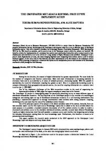
This function outputs a list of all distinct parameter values (t1 , t2 , t3 ) for which there exists a tritangent circle, which is tangent to α(t1 ), α(t2 ) and α(t3 ). 2. CircleCentreVector() The input to this function is a triple (t1 , t2 , t3 ). The function computes the center of the tritangent circle passing through α(t1 ), α(t2 ) and α(t3 ) and its radius. The output given by this function is a vector of reals containing (t1 , t2 , t3 , α(t1 ), α(t2 ), α(t3 ), center, radius). 3. DistanceNearestPoint() The inputs to this function are: • center of a tritangent circle, • der dist- derivative of the distance function computing by using a point and the parametric form of the curve, • SearchInterval: the starting and ending point of the parameter interval of the curve. • Tolerance : the error bound for computing the intervals of the zeros of der dist. This function outputs a real number which is the distance of the center of the tritangent circle from the nearest point on the given curve α. 4. ValidCircle() This function is a boolean function, with the following inputs: • radius of a tritangent circle and • distance to the nearest point from the center of this tritangent circle to the curve. This function outputs True if the radius of the tritangent circle is less than or equal to the distance to the nearest point and False otherwise. 5. CentreIn() This function is a boolean function and the inputs to this function are: • the triple of parameter values (t1 , t2 , t3 ) and • center of the tritangent circle passing through α(t1 ), α(t2 ) and α(t3 ). This function outputs True if the center of the tritangent circle lies to the left of the tangents at α(t1 ), α(t2 ) and α(t3 ) and False otherwise. Figure 1 motivates the function CentreIn(), it shows that for a simple, closed, connected curve in R2 , with a positive orientation, the center of a branching circle, lies to the left of tangents at any for the three points at which the branching circle is tangent to the curve. The algorithm for branch point generation is given by :
8
Figure 1: Every branch point, lies to the left of all tangent lines. Let TripleLst = PruningBifurcationFunction(); For (it == TripleLst.begin(); it ! = TripleLst.end(); it++ ) { vector temp = *it; vector circvec = CircleCenterVector(temp) vector center = (circvec[9],circvec[10]) ; real radius = circvec[11]; real dist = DistanceNearestPoint(center, der dist, SearchInterval, Tolerance); If (ValidCircle(dist, radius)) If (CenterIn(temp,center)) branchPointsLst.push back(temp,center,radius); } Return[branchPointsLst] Hence the list branchPointsLst contains all the branch points of the medial axis of the domain bounded by the given curve α.
3.3
Topology of the medial axis
In the section we outline the main concept of the algorithm behind generating the topology of the medial axis of a given domain Ω, given its leaf and branch points. After finding the leaf points and the branch points, we put all the points in a list alongwith the corresponding parameter values. We see that a leaf point is present once, and a branch point is present thrice, due to three distinct parameter values associated to a branch point. We elaborate this by looking at the example illustrated by Figure 2 From the Figure 2 we see that the parameter values corresponding to the leaf points are given by the list leaf point parameters = {t0 , t3 , t5 , t8 }. Moreover, the parameter values associated with branch points are given by the list branch point parameters = {t1 , t2 , t4 , t6 , t7 , t9 }. Now after sorting the list of all the parameter values, we get the topology list, given by topology lst = {t1 , t2 , · · · , t9 }. Associated to each parameter value is a point on the medial axis, the table below shows this correspondence. From Table 1 we see that two consecutive medial axis points, gives an edge of the medial tree. Where medial tree is tree structure giving the topology of the medial axis. The vertices of the medial tree the leaf and branch points of the 9
t3
t0
t2
t1
t4
t9
t7
t6
t5
t8
Figure 2: Example showing the parameter values corresponding to leaf and branch points param value maxis pts
t0 m0
t1 m1
t2 m2
t3 m3
t4 m2
t5 m4
t6 m2
t7 m1
t8 m5
t9 m1
Table 1: Table giving the parameter values and its corresponding leaf or branch point.
medial axis. The edges of the medial tree help us in generating the parameter intervals required for the tracing algorithm for tracing an approximation of the branches of the medial axis.
4
Implementation Results
The algorithm described so far assumes that the simply connected domain Ω in R2 is bounded by a simple, connected, closed curve given by a single parametrization. We implemented the algorithm for such curves. Moreover we extended the algorithm for spline curves. Our implementation deals with any cubic spline curve which is curvature continuous, or tangent continuous with the assumption that no extremums of the Euclidean curvature exist at the join points. Although our implementation deals with cubic splines only for the time being it can easily be adjusted for any kind of splines with the same assumptions as in the cubic spline case. We implemented our algorithm in C++ using the interval arithmetic library C-XSC1 , for computing the leaf and branch points of the medial axis. We refer to [8] for detailed report on the C-XSC libraries. The tables below show the results on a AMD Athlon(tm) processor with 1.7 GB memory, running Kernel Linux 2.6.22-14-generic. We used the C-XSC 2.2.2 version and GNU C++ compiler gcc 3.4 in all our implementations.
4.1
Results for curves given by single parametrization
In this section we give the results of our implementation for curves given with single parametrization. 1
http://www.xsc.de
10
1. For the curve α : [0, 2 π] → R2 , given by α(t) = ( 13 cos(t) − 81 sin(t), sin(t) − 31 cos(2 t)). Figure 3 gives the result of tracing an approximation of the branches of the medial axis after having found its topology.
Figure 3: Trace of the approximate medial axis
2. Given curve α : [0, 2 π] → R2 , with the parametrization α(t) = (2 cos(t) −
1 6
cos(5 t), sin(t) −
1 6
sin(5 t)).
Figure 4: Trace of the approximate medial axis
3. Let us consider the curve α : [0, 2 π] → R2 , given by the parametrization, α(t) = (7 cos(t) − 2 cos(6 t), 10 sin(t) −
1 3
sin(6 t)).
4. Given a curve α : [0, 2 π] → R2 , with the parametrization, α(t) = (200 cos(t) − 20 cos(20 t), 400 sin(t) − sin(20 t)), the trace of its medial axis is given by Figure 6. In Table 2 we look at the time required for implementing two parts of the algorithm for the curves given by single. The first part called topology combines the computation time for leaf and branch points, together with the time taken to compute the topology of the medial axis. The second part of the implementation, denoted by tracing in the table, is the time taken by the corrector 11
Figure 5: Discretized medial axis
Figure 6: Approximate medial axis
12
algorithm to compute some regular points on the medial axis. Remark 2 We see in the table that the total time for the output for curve 3 is much less than that of curve 2, although the leaf and branch points of curve 3 are more than curve 2. This is due to the fact that the leaf points and branch points in curve 3 are more uniformly distributed over the parameter interval than in case of curve 2. The computation time for curve 2 can be reduced by improving the algorithm where the tolerance is computed on the fly depending upon the distribution of leaf and branch points. curves curve curve curve curve
1 2 3 4
ε 1e−7 1e−5 1e−5 1e−3
Topology Time 37 s 5 min, 12 s 22 s 1 hr, 40 min 13 s
ε 1e−1 1e−2 1e−2 5e−3
Trace Time 7s 1 min, 59 s 39 s 3 min, 33 s
Total Time 44 s 7 min, 11 s 1 min, 1 s 1 hr, 43 min, 46 s.
Table 2: The timing results for curves with single parametrization
4.2
Results of implementation in the spline case
In this section we report some of the results of the implementation of our algorithm in the cubic spline case. In the examples that we give, we list the spline in an anticlockwise order such that they form the boundary of a simply connected domain Ω. Remark 3 To speed up our implementation in the cubic spline case, we use a property of cubic splines. Since each cubic spline can have at most one convex vertex, we have that, a branch point of the medial axis of a closed curve composed of cubic splines would correspond to three distinct cubic splines. 1. Consider the cubic splines α1 (t), · · · α5 (t) : [0, 1] → R2 , Figure 7 shows the approximation of the medial axis of the region bounded by the spline curves. 2. Consider the cubic splines α1 (t), · · · α6 (t) : [0, 1] → R2 , Figure 8 illustrates the approximation of the medial axis of the domain bounded by the spline curves. Table 3 gives the timing result for cubic spline curves shown in Figures 7 and 8 respectively.
5
Conclusion
We compute several examples to test our algorithm. The algorithm is robust, the bottleneck of our algorithm being the computation time taken by the Interval Newton method. We tested our algorithm with two interval arithmetic 13
Figure 7: Approximation of the medial axis of the y-curve
Figure 8: Approximation of the medial axis of the 3-petal curve
14
curves y-curve 3-petal curve
ε 1e−3 1e−3
Topology Time 5 min, 12 s 12 min, 49 s
Trace ε Time −2 1e 0s 1e−2 0 s
Total Time 5 min, 12 s 12 min, 49 s.
Table 3: The timing results for cubic spline curves
libraries C-XSC and ALIAS for the timing results and in all the cases we considered C-XSC gave better timing. Although there are methods presents in ALIAS which can probably reduce the computation time by using their Gradient Method, but in the spline case the expressions for computing the branch points become huge and creates problem with memory when one uses the Gradient of the functions as well. We think that the timing results can be improved upon with some changes in our algorithm together with improvement in the present interval arithmetic libraries. Our algorithm although implemented for cubic splines, can be generalized to other splines as well without changing its logic. Furthermore, to improve the computation time of our implementation for polynomial spline curves, we could use libraries like SYNAPS to compute the roots exactly without using Interval Newton Method. Our algorithm presently although can be used directly for trigonometric splines. Acknowledgements We would like to thank Dr. Simon Plantinga for many helpful discussions about the algorithm and interval arithmetic libraries.
References [1] H. Blum. A Transformation for Extracting New Descriptors of Shape. In Weiant Wathen-Dunn, editor, Models for the Perception of Speech and Visual Form, pages 362–380. MIT Press, Cambridge, 1967. [2] L. Cao and J. Liu. Computation of medial axis and offset curves of curved boundaries in planar domain. Computer Aided Design, 40:465–475, 2008. [3] H. I. Choi, S. W. Choi, and H. P. Moon. Mathematical theory of medial axis transform. Pacific Journal of Mathematics, 181(1):57–87, 1997. [4] W. L. F. Degen. Exploiting curvatures to compute the medial axis for domains with smooth boundary. Comput. Aided Geom. Design, 21(7):641– 660, 2004. [5] I. Z. Emiris, E. P. Tsigaridas, and G. M. Tzoumas. The predicates for the voronoi diagram of ellipses. In Proceedings of the twenty-second annual symposium on Computational geometry, pages 227–236, 2006. [6] G. Evans, A. Middleditch, and N. Miles. Stable computation of the 2d medial axis transform. Internat. J. Comput. Geom. Appl., 8:577–598, 1998. 15
[7] M. Held. On the computational geometry of pocket machining. SpringerVerlag New York, Inc., New York, NY, USA, 1991. [8] W. Hofschuster and W. Kr¨amer. C-XSC 2.0: A C++ Library for Extended Scientific Computing. In Numerical Software with Result Verification, pages 15–35, 2003. [9] D. G. Kirkpatrick. Efficient computation of continuous skeletons. In Proceedings of the 20th Annual IEEE Symposium on Foundations of Computer Science, pages 18–27, 1979. [10] D.T. Lee. Medial axis transformation of a planar shape. PAMI, 4(4):363– 369, July 1982. [11] S. Plantinga. Certified Algorithms for Implicit Surfaces. PhD thesis, University of Groningen, 2007. [12] F. P. Preparata. The medial axis of a simple polygon. Berlin/Heidelberg, 1977.
Springer
[13] R. Ramamurthy and R. T. Farouki. Voronoi diagram and medial axis algorithm for planar domains with curved boundaries. I. Theoretical foundations. J. Comput. Appl. Math., 102(1):119–141, 1999. [14] R. Ramamurthy and R. T. Farouki. Voronoi diagram and medial axis algorithm for planar domains with curved boundaries. II. Detailed algorithm description. J. Comput. Appl. Math., 102(2):253–277, 1999. [15] C. K. Yap. An o (n log n) algorithm for the voronoi diagram of a set of simple curve segments. Discrete & Computational Geometry, 2:365–393, 1987.
16