May 7, 2014 - [34] R. H. Rand, Lecture notes on nonlinear vibrations, ... Holmes, Nonlinear Oscillations, Dynamical Systems, and Bifurcations of Vector Fields, ...
Activating membranes Ananyo Maitra1∗ , Pragya Srivastava2∗† , Madan Rao2,3 and Sriram Ramaswamy4, Indian Institute of Science, Bangalore 560012, India Raman Research Institute, C.V. Raman Avenue, Bangalore 560 080, India 3 National Centre for Biological Sciences (TIFR), Bellary Road, Bangalore 560 065, India 4 TIFR Centre for Interdisciplinary Sciences, Hyderabad 500075, India (Dated: May 9, 2014)
arXiv:1311.5055v2 [physics.bio-ph] 7 May 2014
2
We present a general dynamical theory of a membrane coupled to an actin cortex containing polymerizing filaments with active stresses and currents, and demonstrate that active membrane dynamics [Phys. Rev. Lett 84, 3494 (2000)] and spontaneous shape oscillations emerge from this description. We also consider membrane instabilities and patterns induced by the presence of filaments with polar orientational correlations in the tangent plane of the membrane. The dynamical features we predict should be seen in a variety of cellular contexts involving the dynamics of the membrane-cytoskeleton composite and cytoskeletal extracts coupled to synthetic vesicles.
The plasma membrane of a living cell displays striking dynamical structures in the form of growing tubules, ruffles, ridges, and spontaneously generated waves [1–3]. The generality of these observations prompts us to search for a minimal physical description, independent of system-specific detail, unlike [4, 5]. We show that the essential mechanism lies in the interaction of the membrane with the cytoskeleton, driven by molecular motors and ATP, which can be viewed as a fluid containing orientable, self-driven filaments [6]. Our work is significantly different from a recent paper on membrane waves driven by actin and myosin [7], as we explain in the paper. Our predictions are general, and testable in extracts and artificial settings as well. Our main results: (i) Active membrane dynamics [8–10] emerges naturally from a complete hydrodynamic theory of a membrane forced by a fluid containing orientable motile elements carrying active stresses. The membrane acquires a tension from the intrinsic stresses on the filaments and a sustained normal velocity from their nonequilibrium directed motion. (ii) Within a mode-truncated description, we find an instability to a spontaneously oscillating state. (iii) Including an in-plane polar orientation field in the membrane gives rise to height bands just past the onset of 1/2 spontaneous alignment, travelling instabilities deep in the ordered phase, with growth rate ∼ qx qy , where x is the direction of mean ordering of the filaments, for small in-plane wavevector (qx , qy ), and possibly tubules or ridges in a regime where the polarization focuses onto points or lines. We now construct the dynamics of a fluid membrane coupled to a bulk solvent [11, 13] containing active orientable particles [14] described by a vector order parameter P(r) and a nematic order parameter Q(r), as functions of 3-dimensional position r. The membrane conformation R(~u) is parametrized by ~u = (u1 , u2 ), where ~u is a two dimensional position vector labelling points in the membrane. The local membrane velocity is denoted by Vm (~u, t). If we impose that all surface points labelled by ~u retain their coordinates (i.e. we use a convected coordinate system [15, 16]), Vm ≡ ∂t R. We will work with this choice in the present paper. In [17] we present the general equations for our model. We denote by ψ the “signed” concentration of a species living on or closely associated to the membrane (Fig. 1). That is, each particle of this species has a vectorial orientation, whose axis is taken to lie along the membrane normal, and is counted as + (−) for parallel (antiparallel) alignment. ψ could represent [8] actin polymerization nucleators, asymmetric membrane proteins or ion channels, or an internal state coupling to local curvature [18]. We denote by c the concentration of polar filaments restricted to the immediate vicinity of the membrane. In the cellular context, this represents tangential actin, whose presence has been persuasively argued for in recent studies on membrane composition and trafficking [19]. In the absence of R flow andR activity, the system relaxes to equilibrium governed by a free-energy functional F [P, Q, R, ψ, c] = d3 r(fb + u fm ) with contributions fb from the cytoplasm and fm at the membrane. Here R R ... ≡ d2 ug 1/2 δ(r − R)..., g being the determinant of the membrane metric. fb = (a1 /2)P 2 + (a2 /2)Q : Q controls u the relaxation of the order parameter fields in the bulk. The contributions from the degrees of freedom associated with the membrane are contained in fm = fc + fR + fR−c + fop . Here fc describes the cost of concentration fluctuations of both the in-plane polar filaments and the signed species, and fR = (κ/2)(Tr K)2 penalizes deformations of the membrane, where K is the curvature tensor [20]. fR−c = Υ(c)ψTr K couples the signed density field and the local mean curvature [9]. Lastly, fop = wQu : NN − Λψpn − w2 pn Tr K + ac p~t 2 +αcDu · p~t + κp ψK : (Du p~t ) + κt ψ p~t p~t : K
(1)
is the free-energy associated with orientational order at the membrane: Pu (~u) = P(r = R(~u)) and Qu (~u) = Q(r =
2
FIG. 1: Schematic diagram of a membrane in an active fluid. The membrane is depicted in Monge gauge: R = (x, y, h(x, y, t)) where h(x, y, t) is the height above points (x, y) on a reference plane. The ‘signed’ species ψ is represented by circles with dots (crosses) denoting parallel (antiparallel) alignment with respect to the outward membrane normal N. Dashed arrows on the membrane are the in-plane polar filaments, whose concentration is c, and continuous arrows denote the bulk active orientable fluid.
R(~u)), parametrised by ~u. Du is the covariant derivative on the membrane [15] and N(~u) is the membrane normal. We decompose Pu into its normal component pn = Pu · N and the tangent plane vector p~t = eu · Pu , where the projector eu ≡ (e1 (~u), e2 (~u)) = (∂u1 R, ∂u2 R). The local polarity ψ of the membrane favours one direction of P through Λ, while w, depending on its sign, softly anchors the filaments parallel or perpendicular to the membrane [21]. w2 , κp and κt couple orientation to curvature [22], and ac controls the orientational free energy of membrane-associated tangential polar filaments (hereafter, “horizontal filaments”). The coefficient α governs local spontaneous splay in response to polar filament concentration[23, 24]. In the presence of active processes, the membrane, treated as a permeable fluid film [20], has a local velocity Vm = [V + v0 P + ζ∇ · (PP)]|r=R − µp g −1/2
δF δR
(2)
where V is the three dimensional hydrodynamic velocity. The second and third terms in the square bracket (2), forbidden in a passive system, arise as follows [6]: free energy is dissipated at a rate R∆µ, where R is the reaction rate and ∆µ the chemical potential difference between the fuel (e.g., ATP) and its reaction products. Let us treat Vm and R as fluxes [25, 26], with corresponding forces δF/δR and ∆µ. To first order in gradients, P and ∇ · (PP), measuring local polarity, contribute terms of the form ζ1 P·δF/δR and ζ2 ∇·(PP)·δF/δR to R, where the independent kinetic coefficients ζ1 and ζ2 vanish for an impermeable membrane, as does µp . The symmetry of dissipative Onsager coefficients then implies terms ζ1 ∆µP ≡ v0 P and ζ2 ∆µ∇ · (PP) ≡ ζ∇ · (PP) in the Vm equation. In the cellular context v0 is the scale of the drift speed of the membrane arising from filament polymerization [27]. The signed density field ψ has a dynamics given by Dt ψ = −Du · J~ − k2 ψ + k1
(3)
where Dt is the covariant time derivative, and k1 , k2 are rates of association and dissociation to the membrane. The current � � �� δF J~ = J~0 ≡ −ψeu · ∂t R − D ψDu g −1/2 , (4) δψ contains drift and diffusion; the diffusivity D can include R active contributions. The Stokesian hydrodynamic Rvelocity field V(r) = r0 H(r − r0 ) · F(r0 ), where H(r0 ) is the Oseen tensor [28]. The force density F(r, t) = ∇ · σ Q + u δF/δR, where the order parameter stress [29] σ Q has an active contribution of the form ζQ Q [30, 31]. ˙ = λ0 S − ΓQ δF/δQ, where S is ˙ = −Γp δF/δP and Q The order parameters have standard equations of motion [6] P
3 the symmetrised velocity gradient tensor. The local dynamics of the membrane on scales small compared to the whole cell can be understood in the Monge gauge (Fig. 1), R = (x, h(x, t)), g = 1 + (∇⊥ h)2 and N = g −1/2 (−∇⊥ h, 1), where h(x) is the height of the membrane above a point x on the reference plane. We first concentrate on the coupled dynamics of h and ψ in an isotropic bulk phase with negligible c. On long time-scales the order parameters relax to values governed by their coupling to the membrane which, to lowest order in gradients, are Pu = ψ
Qu =
Λ N, a1
(5a)
ΓQ λ0 w S|r=R − (NN − I/3). a2 a2
(5b)
Using these expressions for P and Q in (2), (3) and (4) leads to the coupled equations
∂t h = g 1/2 [˜ v ψ − µp
δF ]− δh
Z q
eiq⊥ ·x
1 δF 2 (γact q⊥ hq + ) 4˜ η q⊥ δh
∂t ψ = v˜∇⊥ · (g −1/2 ψ 2 ∇⊥ h) + D∇⊥ · [ψ∇⊥ (g −1/2
δF )] − k2 ψ + k1 δψ
(6a)
(6b)
in which the active stress contributes a tension γact = −ζQ w/a2 (see [21] for a one-dimensional analogue) and, as in [32], a modified viscosity η˜ = η + (−λ0 a2 + ζQ )ΓQ λ0 /a2 . We have not included the effects of the active term with the coefficient ζ defined in (2). The lowest order term it contribues to the height equation is ∇2⊥ h, i.e. an active non-hydrodynamic tension. Its more crucial consequences are examined later on in the paper Note that the active modification of the hydrodynamic tension is missing in [10], where the force dipoles are taken to be situated at the reference rather than the actual location of the membrane. Local polarity leads to the propulsion of the membrane at a rate ψ˜ v = ψv0 Λ/a1 . F in (6a) and (6b) is the original free-energy functional with P and Q eliminated in favour of ψ and h via (5a) and (5b) respectively. The first term on the right-hand side in (6b) arises kinematically, due to the change of density of an in-membrane species resulting from a change in the conformation of the fluid film[20]. Setting k1 and k2 to zero to specialise to the case of a zero mean conserved species, eqns. (6a) and (6b) take precisely the form presented [9] on general grounds for an active membrane [33]. This establishes one of our main results: a membrane in an active fluid is an active membrane, propelled by polar activity – polymerization, in the context of actomyosin – with a tension from contractility. Equations (2) - (6) with suitable boundary conditions can be applied to cell membranes or reconstituted systems. The terms proportional to v˜ in (6) constitute an excitatory-inhibitory pair which, we now show, leads to sustained spontaneous oscillations in a regime of parameter space. We work in one dimension, retaining only the smallest wavenumber and only one nonlinear term: ∇⊥ · (ψ 2 ∇⊥ h) in (6b). The resulting coupled ODEs [17] upon re-scaling and defining new constants describe a generalized Van der Pol oscillator with a linear damping and cubic nonlinearities: ˙ 2 + s4 φ3 = 0 φ¨ + φ + s1 φ˙ + s2 φ2 φ˙ + s3 φ(φ)
(7)
which has been shown [34] to have a limit cycle if sgn(s1 s2 ) = −1. We provide further details regarding the mode truncation and present a representative phase portrait in the supplement [17]. Note that wave-like dispersion relations as in [7, 35] are distinct from the experimentally observed membrane waves [2, 3], which are not a response to an external perturbation, but are self-generated, in a manner consistent with our findings from the truncated model. Moreover, the wave-speed in our theory is set solely by the normal drift speed, not by free-energy couplings. Our analysis of (6) suggests an explanation for the experimentally observed waves [2, 3] on the lamellipodium [36] of a crawling or spreading cell, whose leading edge should be viewed as an actively moving one-dimensional membrane. We expect similar waves on the surface of self-propelled drops [37] e.g., in parameter regimes corresponding to the instability discussed in [9], which arises here if v˜Υ > 0. In the case we present here and in [17] actin polymerization, not contractility, is the proximate cause of the membrane waves [3]. Note: even without permeability, a local normal velocity at the membrane, proportional to |q⊥ |ψq , which can be shown to arise from an active contractile stress, can generate spontaneous waves with dispersion ω 2 ∼ q 3 [10, 17]. Now we examine another case of importance to cell biology, in which a distinct population of filaments, lying in
4 the vicinity of the membrane and disposed parallel to it, are present at sufficient concentration for their dynamics to be slow and therefore relevant on the timescale of interest to this work. This is motivated by experimental studies [19] of the nanoclustering of cell-surface molecules, whose anomalous statistical properties are naturally accounted for as arising from active transport mediated by a new class of “horizontal actin filaments”. We study the effect of such tangential active orientable filaments on membrane fluctuations, and make predictions which can be tested in future experiments. For this, we introduce a separate dynamical equation for the polar order parameter Pu at the membrane [20]: Dt Pu − (eu · ∂t R) · Du Pu + vp p~t · Du Pu = −g −1/2 Γp δF/δPu
(8)
where vp is the self-propulsion velocity [38]. In the following treatment, for simplicity, we replace hydrodynamic damping by local friction with respect to a fixed background medium. We assume the horizontal filaments are close to an ordering transition but take the normal component pn to relax rapidly. To the lowest order in gradients, (5a) implies pn = (Λ/a1 )ψ. The equation for the tangential component is 1 δF Dt p~t − eu · [(eu · ∂t R) · Du Pu ] + vp eu · (p~t · Du Pu ) = − √ Γp eu · + (Dt eu ) · Pu , g δPu
(9)
Conservation of horizontal filaments implies Dt c = −Du · (c~vc ) + Dc Du · [cDu (g −1/2
δF )], δc
~vc = −eu · ∂t R + v1 p~t .
(10a)
(10b)
The membrane conformation is given by (2), while the current of ψ in (3) is modified to J~ = J~0 + vψ p~t . v1 and vψ are active polar velocity parameters, independent of each other and of vp in (8). Eqs. (2), (3), (9) and (10) are a formally complete description of the dynamics of a membrane endowed with inplane polar orientational order and signed species coupled to active ‘horizontal’ and ‘vertical’ filaments. A complete exploration of the range of behaviors of this system requires a numerical study. We limit ourselves here to a linear stability analysis about the isotropic and in-plane ordered states in a steadily moving membrane which is flat on average. This is the regime in which dynamics of ψ is fast and relaxes to a steady state value ψ0 = k1 /k2 , (3). As k2−1 ∼ 0.1 − 1s [39] our assumption is justified if we are looking at the dynamics on timescales greater than 1s. We re-scale our equations so that ψ0 = 1. The coupled equations of the height field h, the in-plane component of the polar order parameter p and concentration c, to leading order in gradients, are
∂t h = v˜(c) +
ζ ∇⊥ · [Λ(c)p] + µp [Σ∇2⊥ h − κ∇4⊥ h + ∇2⊥ Υ(c) − κp ∇2⊥ ∇⊥ · p − κt ∇⊥ ∇⊥ : pp], a1
∂t p = −vp p · ∇⊥ p +
v˜(c)v0 ˜ + κp ∇⊥ ∇2⊥ h + α∇⊥ c − κt p · ∇⊥ ∇⊥ h] + Dp ∇2⊥ p ∇⊥ Λ(c) + Γp [−Ap a1 ∂t c = ∇⊥ · [c(v1 p + v˜(c)∇⊥ h)] + Dc ∇2⊥ c,
(11a)
(11b)
(11c)
where ∇2⊥ Υ(c) arises from the free energy contribution fR−c . Σ in (11a) is an active tension [9], arising, for R example, via an interplay of the active polymerization and the polar anchoring modelled by the free-energy cost − u w2 pn Tr K in (1). This coupling generates a term of the form ∇2⊥ h in the pn equation and, therefore, because of propulsion, an effective tension in the h equation. (11b) was obtained by projecting (9) onto the reference horizontal, with A˜ = (ac + a1 ). The term with coefficient Dp arises from the Frank elasticity of the polar filaments. Note the absence of a term proportional to ∇⊥ h in (11b), a consequence of three-dimensional rotation invariance [11]. The propulsive velocity v˜ in (11) is taken to depend only on c as ψ has been set to a constant value. We turn next to some original instability mechanisms emerging from (11). ˜ p is then deep in the isotropic phase, and can thus be eliminated in favour First consider the case of large positive A.
5 of h and c on timescales long compared to its finite relaxation time. The resulting equations are then those of [9], with ˜ The complete problem, including the dynamics of p, is characterized by two a modified diffusivity Dc → Dc + αv1 /A. eigenmodes with relaxation rates ∼ q 0 and two of order ∼ q 2 , unaffected to leading order in q by the coupling ∇⊥ ∇2⊥ h in the p equation. A large enough negative α leads to an instability with aggregation of c and modulation of h. This picture is borne out by a linear stability analysis in which the dynamics of p is retained [17], revealing an eigenvalue of order q 2 that changes sign for sufficiently large negative αv1 . The projection of the corresponding eigenvector onto h grows with increasing v˜. The underlying process involves the focusing of p and hence the concentration, leading, through the v˜(c) term in (11a), to growth of the height field. Whether the focusing of p takes the form of asters or walls, leading respectively to height modulations in the form of tubules or ridges, requires a numerical calculation. If both A˜ and α are negative, an extrapolation of the results of [24] would suggest the formation of ordered modulations of h. In flocking models [40], just past the onset of the ordered phase of p, the coupled dynamics of c and p gives rise, ˜ to a state with travelling bands of concentration [41]. In the present context where through the c dependence of A, the dynamics takes place on a membrane this should be accompanied, through v˜(c) in (11a), by a one-dimensional fore-aft asymmetric modulation of the membrane height. The coupled dynamics of p and h with c fixed shows a distinct class of modes and instabilities deep in the regime 1/2 where p is ordered. For vp = 0 there is a travelling instability with relaxation rate of transverse fluctuations ∼ qy qx , 2 if the ordering direction is taken along x. As vp is increased this crosses over to ∼ qy [17]. Note, despite the similarity of form with the mode structure of [12], that the detailed mechanisms are different. To summarize: we have shown that the equations of motion for an active membrane [9] emerge from the dynamics of an ordinary fluid membrane coupled to a medium with active, motile filaments. We find that the resulting equations display spontaneous sustained oscillations driven by the active motion of the membrane normal to itself which are the natural explanation of membrane waves [2, 3]. In addition, when polar “horizontal filaments” [19] are included, the coupled dynamics of their concentration and orientation and the membrane height leads to instabilities towards oneor two-dimensional modulations, as well as travelling undulations. Deep in the orientationally ordered phase of the filaments we find propagating instabilities with singularly anisotropic dependence on wavevector. Ongoing numerical studies of the long-time dynamics emerging from these instabilities find a varied range of behaviors including stable tubules and spatiotemporal chaos [42]. Meanwhile, we look forward to tests of our predictions in actomyosin extracts with ATP and actin nucleators in contact with model lipid membranes.
Acknowledgments
AM and SR thank Jean-Fran¸cois Joanny for useful discussions in the early stages of the work. AM, PS and MR thank TCIS, TIFR Hyderabad for hospitality, and SR acknowledges a J.C. Bose fellowship. MR acknowledges a grant from Simons Foundation. ∗ Equal contributors † Present address: Physics department, Syracuse University, Syracuse, NY-13244, USA
[1] J. Allard and A. Mogilner, Curr. Op. Cell Bio. 25, 1 (2012). [2] C. H. Chen, F. C. Tsai, C. C. Wang, C. H. Lee, Phys Rev Lett. 103, 238101 (2009). [3] H. G. D¨ obereiner, B. J. Dubin-Thaler, J. M. Hofman, H. S. Xenias, T. N. Sims, G. Giannone, M. L. Dustin, C. H. Wiggins, M. P. Sheetz, Phys Rev Lett. 97, 038102 (2006). [4] K. Doubrovinski, K. Kruse, Phys. Rev. Lett. 107, 25 (2011). [5] A. Gholami, M. Enculescu, Martin Falcke, New J. Phys. 14, 115002 (2012). [6] M. C. Marchetti, J. F. Joanny, S. Ramaswamy, T. B. Liverpool, J. Prost, M. Rao and R. A. Simha, Rev. Mod. Phys. 85, 1143 (2013). [7] R. Shlomovitz, N.S. Gov, Phys. Rev. Lett. 98, 168103 (2007). [8] J. Prost and R. Bruinsma, Europhys. Lett. 33, 321 (1996); S. Ramaswamy, J. Toner, and J. Prost, Pramana 53, 237 (1999); S. Ramaswamy and M. Rao, C. R. Acad. Sci. Paris, S´erie IV 2, 817 (2001). [9] S. Ramaswamy, J. Toner, and J. Prost, Phys. Rev. Lett. 84, 3494 (2000). [10] J-B. Manneville, P. Bassereau, S. Ramaswamy, J. Prost, Phys. Rev. E 64, 021908 (2001). [11] No substrate is present to provide a fixed reference horizontal, unlike in [12]. [12] S. Sankararaman, S. Ramaswamy, Phys. Rev. Lett. 102, 118107 (2009). [13] Our boundary conditions and geometry differ from those of N. Sarkar, A. Basu, Eur. Phys. J. E 35, 115 (2012), ibid. 36, 8 (2013).
6 [14] We ignore the fluctuations of the concentration of the filaments in the bulk fluid. [15] R. Aris, Vectors, Tensors and the Basic Equations of Fluid Mechanics, Dover, USA (1989). [16] D. Hu, P. Zhang, Phys. Rev. E 75, 041605 (2007). [17] Supplementary material [18] H.-Y. Chen, Phys. Rev. Lett. 92, 168101 (2004). [19] D. Goswami, K. Gowrishankar, S. Bilgrami, S. Ghosh, R. Raghupathy, R. Chadda, R. Vishwakarma, M. Rao, and S. Mayor, Cell 135, 1085 (2008); K. Gowrishankar, S. Ghosh, S. Saha, Ruma, C., S. Mayor, M. Rao, Cell 149, 1353 (2012). [20] W. Cai, T. C. Lubensky, Phys. Rev. E 52, 4251 (1995). [21] N Kikuchi, A Ehrlicher, D Koch, J A Kaes, S Ramaswamy, M Rao, Proc. Natl. Acad. Sci. 106, 19776 (2009). [22] T. Powers and P. Nelson, J. Phys. II 5, 1671 (1995). [23] W. Kung, M. C. Marchetti and K. Saunders, Phys. Rev. E 73, 31708 (2006); R. C. Sarasij, S. Mayor, and M. Rao Biophys. J. 92, 3140 (2007). [24] K. Gowrishankar and M. Rao, arXiv:1201.3938 (2012). [25] S. R. de Groot, P. Mazur, Non-Equilibrium Thermodynamics (Dover Books on Physics). [26] F. J¨ ulicher, K. Kruse, J. Prost and J.-F. Joanny, Phys. Rep. 449, 3 (2007). [27] C. Sykes, J. Prost, and J.F. Joanny, in Actin-based Motility: Cellular, Molecular and Physical Aspects, Carlier, MarieFrance (Ed.), Springer, New York (2010). [28] J. Happel, H. Brenner, Low Reynolds number hydrodynamics: with special applications to particulate media (Springer). [29] P. G. de Gennes, J. Prost, The Physics of Liquid Crystals (second edition), Clarendon, Oxford (1993). [30] Other active terms, bilinear in P, are present but do not matter in the subsequent analysis. [31] There can be no monopole term in the force density because of momentum conservation. Such a term is introduced in [7], but its presence is thereafter rendered innocuous once the authors replace hydrodynamic damping by local friction. [32] Y. Hatwalne, S. Ramaswamy, M. Rao and R. A. Simha, Phys Rev Lett 92, 118101 (2004). [33] Activity can also renormalise the bending rigidity through the interplay of the lowest order polar active term in the stress, R ∇P + (∇P)T , and an allowed free energy coupling, u w2 ∇P : NN. [34] R. H. Rand, Lecture notes on nonlinear vibrations, http://ecommons.cornell.edu/handle/1813/79; J. Guckenheimer and P. Holmes, Nonlinear Oscillations, Dynamical Systems, and Bifurcations of Vector Fields, Springer-Verlag, New York (1983). [35] N. S. Gov, A. Gopinathan Biophys. J. 90, 454 (2006). [36] J. V. Small, T. Stradal, E. Vignal, K. Rottner, Trends Cell Biol. 12, 112 (2002). [37] E. Tjhung, D. Marenduzzo, and M. E. Cates, Proc. Natl. Acad. Sci. 109, 12381 (2012). [38] We ignore other possible terms at this order in gradients and fields [40] which do not play a significant role here. [39] T. D. Pollard, G. G. Borisy, Cell 112, 453 (2003). [40] J Toner, Y Tu Phys. Rev. Lett. 75, 4326 (1995); J. Toner, Y. Tu, Phys. Rev. E 58, 4828 (1998); J. Toner, Y. Tu and S. Ramaswamy, Ann. Phys. 318, 170 (2005). [41] E. Bertin, M. Droz, G. Gr´egoire, Phys. Rev. E 74, 022101 (2006); H. Chat´e, F. Ginelli, G. Gr´egoire, Guillaume and F. Raynaud, Phys. Rev. E 77, 046113 (2008); E. Bertin, M. Droz, G. Gr´egoire, J. Phys. A: Math. Theor. 42, 445001 (2009); S. Mishra, A. Baskaran, M. C. Marchetti, Phys. Rev. E 81, 061916 (2010). [42] A. Pande, A. Maitra, S. Ramaswamy, R. Pandit, to be submitted; A. Pande, Ph D thesis, Indian Institute of Science (2000).
7 Activating Membranes; A. Maitra et al. : Supplementary Material
In this supplementary, we provide (i) intermediate steps for derivation of the Eqn. (7) in the main text, starting from the equations describing active membrane (Eqn.(6) in the main text) along with the phase portrait showing the limit cycle, (ii) explanation of the oscillatory state in an impermeable membrane and (iii) expressions and plots of dispersion relations for a membrane with an in-plane polar order parameter.
A.
Derivation of the membrane equations
In this section we present the full time-dependent reparametrisation invariant equations for our model. Let ρ be the mass density of the membrane. It follows an equation of motion Dt ρ + Du · (ρ~v ) = 0
(12)
Vm = ~v · eu + ∂t R
(13)
where ~v is the membrane velocity field.
where contraction on the two-dimensional index of eu is used here to “lift” ~v to three dimensions. In general, the mobility relating of the membrane with respect to the fluid is anisotropic with the friction being different normal and tangential to the membrane. In (2) of the main paper we looked at the special case of an isotropic mobility. The general expression corresponding to (2) of the main paper is ˜ · (PP)|r=R − µ˜p g −1/2 Vm = V|r=R + M · [˜ v0 P|r=R + ζ∇
δF ] δR
(14)
where M is an anisotropic mobility. With this formulation one can consider various cases for the membrane-bulk fluid interaction like no-slip in the tangential direction or no-penetration in the normal one. For instance, no-slip condition can be imposed as eu · Vm = eu · V|r=R , i.e. the tangential friction is infinite. In this case, ~v = eu · V|r=R − eu · ∂t R. As in [5], (14) can be transformed into an equation for normal fluctuations of the membrane ∂t R · N and conservation law for density using (12) to eliminate ~v . The dynamical equation for ψ is � � �� u u −1/2 δF Dt ψ = Du · (ψe · ∂t R) − Du · (ψe · V|r=R ) + DDu · ψDu g (15) δψ When the tangential filaments are also included, the equation is modified to � �� � δF Dt ψ = vψ Du · (ψ~ pt ) + Du · (ψeu · ∂t R) + DDu · ψDu g −1/2 δψ
(16)
˙ ⊥ h because of When these equations are expressed in Monge gauge, the current of ψ has a term proportional to ψ h∇ metric fluctuations, which gives rise to the kinematic term in eq. (6b) of the main paper. The dynamical equation for the concentration of tangential filaments � � �� δF Dt c = v1 Du · (c~ pt ) + Du · (ceu · ∂t R) + Dc Du · cDu g −1/2 . (17) δc The polarisation vector follows the equation Dt Pu − (eu · ∂t R) · Du Pu + vp p~t · Du Pu = −g −1/2 Γp δF/δPu This constitutes a complete set of equations for our model.
(18)
8 B.
Full expressions for the order parameter equations and the hydrodynamic stress stensor
Consider a suspension of active particles in a fluid. The particle phase velocity vp in such systems is given by vp = ζ1 P + ζ2 ∇ · Q + v + ...
(19)
where v is the centre of mass velocity, and ζ1 and ζ2 are arbitrary activity parameters. The ellipsis denotes the higher order contributions to vp arising from the particle phase stress. The three-dimensional polar order parameter has the following equation of motion [1] δF ∂t Pi = −vjp ∂j Pi − λpijk ∂k vjp + λ˜p ∂j ∂j vip − ΓP ij δPj
(20)
λpijk describes alignment of the polarisation vector with gradients in velocity. A polarisation vector can also reorient to point along the gradient of strain-rate through the term with coeffcient λ˜p . λpijk =
1−λ T Pi Pj Pk T T (δij Pk + δik Pj + δjk Pi ) + λ 2 P2
(21)
with T δij = δij −
Pi Pj P2
(22)
and ΓP ij = Γp δij + Γ1 Pi Pj + Γ2 (∂i Pj + ∂j Pi )
(23)
to second order in gradients and fields. The apolar order parameter is governed by the following dynamical equation [2]: ∂t Qij =
−vkp ∂k Qij
+
λijkl ∂l vkp
−
ΓQ ijkl
�
δF δQkl
�ST (24)
We define AST to be the symmetrised traceless part of any tensor A . λijkl =
2 1 λ0 (δik δjl + δjk δil − δij δkl ) + (δik Qjl − δil Qjk + δjk Qil − δjl Qik ) 2 3 2 λ1 4 + (δik Qjl + δjk Qil + δjl Qik + δil Qjk − δij Qkl ) + λ2 Qij Qkl 2 3
(25)
and ΓQ ijkl =
ΓQ (δik δjl + δil δjk + δjl δik + δjk δil ). 4
(26)
We define the strain rate tensor as Sij = 1/2(∂i vj + ∂j vi ) − 1/3∇ · vδij . The order parameter equations presented in the main paper are lowest order in gradients and fields versions of these when there is no global orientational order. The description retaining both P and Q merits some comment. In the phase in which P globally orders along a certain direction, obviously Q has a steady state value Qij ∝ Pi Pj − (1/3)δij P 2 . The fluctuation equation that one writes down for Q is for deviations away from this state. It is not completely determined by the fluctuations of the P. Moreover, the polar and apolar order may develop independently, e.g., in the sequence isotropic → apolar → polar, in a system in which the individual orientable particles were polar. Also, the presence of a signed species in the membrane can promote local polar ordering even in the parameter regime in which bulk apolar ordering is preferred. Lastly, we neglect terms of the form Pi Pj in the Qij equation of motion, and Qij Pj in the Pi equation, which do not affect our conclusions in any essential way as we are expanding about a bulk isotropic fluid. We will now explicitly write down the full order-parameter stress tensor σ Q for our model. The active contribution is σaQ = ζQ Q + ζP PP + ζ˜P [(∇P + (∇P)T ]
(27)
9 The activity parameters ζQ , ζP and ζ˜P are functions of local concentration of the filaments. There can also be active contributions to the pressure. However, such terms do not play any role in our model due to incompressibility. The passive contributions to the order-parametr stress to polar and apolar order parameter are, respectively � � δF δF ∂f p δF Q p ˜ − λijk + λ ∂i + ∂j (28) σpolar = ∂i Pk ∂(∂j Pk ) δPk δPj δPi
Q σapolar = −(∂i Qkl )
� �ST ∂f δF − λklij ∂ (∂j Qkl ) δQkl
(29)
From the above expression of the order parameter stress we see that in the disordered phase the only relevant active contribution is through ζQ . C.
Derivation of equation (7) from equation (6)
Eqn. (6) of the main text in one dimension, if one ignores all non-linearities except ∇⊥ · (ψ 2 ∇⊥ h) in (6b), is Z 1 2 4 2 eiqx x ∂t h = v˜ψ + Σ∂x h − µp κ∂x h − µp κ0 ∂x ψ − γact qx2 h (30a) 4˜ η qx qx ∂t ψ = v˜∂x (ψ 2 ∂x h) + D∂x2 ψ − κ0 ∂x4 h − k2 ψ + k1
(30b)
The presence of the Σ term will be argued for later in the paper. These equations with Neumann boundary conditions in an interval of length π, retaining only the smallest wavenumber (q = 1), read
Here, m1 = v˜ + µp κ0 , m2 = Σ + µp κ +
d h1 = m1 ψ1 − m2 h1 dt
(31)
d ψ1 = −m3 (ψ1 ψ1 h1 ) − m4 ψ1 − m5 h1 . dt
(32)
γact 4η ;
m3 = v˜; m4 = D; and m5 = κ0 . These equations have eigenvalues
−(m2 + m4 ) [(m2 − m4 )2 − 2m1 m5 ]1/2 ± 2 2
(33)
We can combine (31) and (32) into one second order differential equation, which upon defining φ = (m5 + m2 m4 )h p and τ = (m5 + m2 m4 )t, yields ˙ 2 + s4 φ3 = 0 φ¨ + φ + s1 φ˙ + s2 φ2 φ˙ + s3 φ(φ)
(34)
where an overdot denotes a derivative with respect to τ . This is a generalised Van der Pol oscillator [3] with a linear damping and cubic nonlinearities, with new constants related to mi as follows: s1 = √
s2 =
m2 + m4 m5 + m2 m4
(35)
2m3 m2 m1 (m5 + m2 m4 )5/2
(36)
m3 (m5 + m2 m4 )2
(37)
s3 =
10
FIG. 2: A representative phase portrait showing a stable limit cycle. The chosen parameter values are s1 = −1, s2 = 2.5, s3 = 0.5, and s4 = 1. The limit-cycle is formed through a supercritical Hopf bifurcation. [4]
s4 =
m3 m22 m1 (m5 + m2 m4 )3
(38)
We present a representative phase portrait in Fig. 2for this equation which shows a limit cycle. Note that this analysis is independent (except for the value of m2 ) of whether the membrane fluctuates in a fluid or with respect to a fixed background medium. The main difference between the two cases is the absence, in the second case, of a damping term linear in wavevector. In a mode-truncated description, this detail does not change the conclusion about the presence of an oscillatory state.
D.
The h − ψ excitatory-inhibitory coupling in an impermeable membrane
The coupled eqs. (2) and (3) of the main text, in Monge gauge, imply that ∂t ψ will have a term proportional to ∇⊥ · (ψvn ∇⊥ h) due to kinematic reasons, where vn ≡ Vm · N. In an impermeable membrane, with no-slip in the tangential directions Vm = V|r=R
(39)
where V(r) = r0 H(r − r0 ) · ∇ · σ(r0 ), with σ being the hydrodynamic stress tensor. The lowest order polar active term in σ is ζp [∇P + (∇P)T ]. Integrating out P using eq. (5a) of the main text, we obtain Z 1 ζp Λ 2 vn = − eiq⊥ ·x q ψq (40) 4˜ η q⊥ a1 ⊥ q R
from the polar stress. Thus, the kinematic term in the dynamical equation for ψ is Z 1 ζp Λ ∇⊥ · (ψ∇⊥ h eiq⊥ ·x |q⊥ |ψq ). 4˜ η q⊥ a1 q⊥
(41)
Let us assume the system is in a noisy stationary state, either as a result of intability and chaos or because of the presence of thermal or chemical noise. We can then replace the pair of ψ fields by their pair correlation in a kind of Hartree approximation. Thus, (41) becomes Z 1 ζp Λ ∇⊥ · (∇⊥ h ei(q⊥ +k)·x |q⊥ | < ψk ψq >) (42) 4˜ η q⊥ a1 q⊥ ,k R Defining < ψk ψq >= Gq δ(q⊥ + k), we see that the integral in (42) reduces to q |q⊥ |Gq . Thus, as long as Gq is not qR highly singular as q⊥ → 0, we obtain waves with dispersion ω 2 ∼ q 3 and speed ζp Λ/(4˜ η q⊥ a1 ) q |q⊥ |Gq . Note that the presence of the active polar stress is not a neccessary requirement for an active impermeable membrane to oscillate. If we consider an allowed free energy coupling ψQt : K, where Qt = eu eu : Q with eu defined below eqn
11
FIG. 3: Plot of the real part of the largest eigenvalue as a function of |q| for α = −3.1 (blue continuous line), and α = −2.1 (red dashed line). All other parameter values are 1
(1) of the main text, and integrate out Qt to obtain Z Qt ∼
ψK,
(43)
u
we find Z vn ∼ − q
eiq⊥ ·x
1 2 q ψq 4˜ η q⊥ ⊥
(44)
because of the active apolar stress. The argument presented in the previous paragraph, for spontaneously generated waves on the membrane, then follows through.
E.
Dispersion relations for coupled dynamics of p and h
Eqns.(11) in main text describe the coupled dynamics of membrane shape and concentration and polar orientation of horizontal actin filaments. Here we discuss the linear stability of this system. For A˜ > 0, i.e. when the orientation correlations of the polar filaments decay exponentially with distance, there are two modes with eigenvalues ∼ q 0 and two with eigenvalues ∼ q 2 , unaffected, to leading order in wave-numbers, by the ∇⊥ ∇2⊥ h coupling in p. The absence of a linear coupling of h to p, at lower order in gradients, is ultimately a consequence of three-dimensional rotation invariance. Defining φ = ∇⊥ · p, the system of linearised equations in the isotropic phase is −Σq 2 v˜ ζΛ0 /a1 h h v q 2 −Dc q 2 v1 c , ∂t c = −˜ (45) φ φ 0 −αq 2 −Γp A˜ where Λ0 = Λ(c0 ), c0 being the mean concentration of the polar filaments. The eigenvalues, Ω, of this set of equations are the solution of the equation Ω3 + m1 Ω2 + m2 Ω + m3 = 0, m1 = (Σ + Dc )q 2 + Γp A˜ ˜ 2 + v˜2 q 2 + αv1 q 2 + Dc Σq 4 m2 = (Σ + Dc )Γp Aq
(46)
12 ˜ 2 + Dc ΣΓp Aq ˜ 4 + Σαv1 q 4 − ζΛ0 v˜α/a1 q 4 . m3 = v˜2 Γp Aq with a general solution whose complicated form is not particularly enlightening. However, if other parameters are held fixed, we see that the eigenvalue with the maximum real part becomes positve as αv1 becomes large and negative (Fig. 3). The corresponding eigenvector has a large projection on h, which increases with increasing value of v˜. The instability can be easily understood if the φ field is integrated out: it arises from the effective diffusivity in the c equation becoming negative, and the resulting unbounded growth in local concentration promoting modulation of the membrane height. We now provide the expressions of the eigenvalues of the stability matrix. We will perturb about a state with a q ˜
ˆ ≡ p0 x ˆ, where β is the coefficient of the P 4 term in the free energy. The transverse fluctuations of mean p0 = A βx the order parameter, py , and the height field fluctuations are hydrodynamically slow in this phase. The general mode structure is quite complicated, with eigenvalues
Ω1,2 =
1 [−ivp p0 qx − (µp Σ + Dp )q 2 − κµp q 4 ] 2 1 ± [−b4 qx2 + b3 qx2 qy2 + b2 q 2 qy2 + b1 q 4 − b6 q 4 qy2 − b5 q 6 + b7 q 8 + i(b8 qx q 2 + b9 qx qy2 − b10 qx q 4 )]1/2 2
(47)
with the coefficients bi defined as b1 = (Dp − µp Σ)2 b2 = 4Γ−1 p κp ζΛ0 /a1 2 2 b3 = 4Γ−1 p µp κt p0
b4 = vp2 p20 b5 = 2κ(Dp − µp Σ) 2 b6 = 4Γ−1 p µp κp
b7 = κ2 µ2p b8 = 2vp p0 (Dp − µp Σ) b9 = 4Γ−1 p κt p0 ζΛ0 /a1 b10 = 2κµp vp p0 The mode structure for small wavevectors transverse to the ordering direction (i.e qx = 0, qy → 0) is
Ω1,2
" # 2 2Γ−1 1 1 p µp κp − κ(Dp − µp Σ) 2 −1 1/2 2 κµp ± qy4 (48) = − [(µp Σ+Dp )±[(Dp −µp Σ) +4Γp κp ζΛ0 /a1 ] ]qy − 1/2 2 2 [(Dp − µp Σ)2 + 4Γ−1 p κp ζΛ0 /a1 ]
We observe that these modes become propagative if ζ is large and negative. For ζ > 0 the ordered state becomes unstable even with a stabilising tension. We plot a stability diagram for this mode in Fig. 4
13
FIG. 4: Stability diagram for transverse fluctuations of a homogeneously polarized phase. I : stable membrane, II : decaying waves, III : oscillatory instabilitiy and IV : instability with ∼ q 2 dispersion.
The mode structure for wavevectors along the ordering direction is 1 Ω1 = −ivp p0 qx − (Dp + µp Σ)qx2 2
(49a)
1 Ω2 = − (Dp + µp Σ)qx2 2
(49b)
1/2
Now we examine the instability with the growth rate qx qy as mentioned in the main text. This instability which arises from the combination of activity ζ and curvature coupling κt [see equations (11) of main text], is best seen in the limit of immotile particles i.e. vp = 0. In this limit, the mode structure, to leading order in wavevectors, is ! 1 + i sgn(ζΛ0 κt qx ) 4κt Γ−1 p p0 ζΛ0 √ Ω1,2 = ± qx1/2 qy (50) a1 2 Since Ω1,2 have real and imaginary parts, the mode displaying the instability travels in a direction governed by sgn(ζΛ0 κt ). If the particles are slightly motile, i.e. with vp which is smaller than the other velocity scales in the problem, the mode structure, to leading order in gradients and vp is Ω1 = 2
κt ζΛ0 2 q Γp vp a1 y
Ω2 = −ivp p0 qx − 2
κt ζΛ0 2 q Γp vp a1 y
(51a)
(51b)
We see that the instability is weakened with increasing motility, another feature in common with [6].
[1] W. Kung, M. C. Marchetti and K. Saunders, Phys. Rev. E 73, 31708 (2006). [2] H. Stark, T. C. Lubensky, Phys. Rev. E 67, 061709 (2003). [3] R. H. Rand, Lecture notes on nonlinear vibrations, http://ecommons.cornell.edu/handle/1813/79; J. Guckenheimer and P. Holmes, Nonlinear Oscillations, Dynamical Systems, and Bifurcations of Vector Fields, Springer-Verlag, New York (1983). [4] This figure was created using pplane 8 developed by John C. Polking. http://math.rice.edu/ dfield/dfpp.html. [5] W .Cai, T. C. Lubensky, Phys. Rev. E 52, 4251 (1995). [6] S. Sankararaman, S. Ramaswamy, Phys. Rev. Lett. 102, 118107 (2009).