To appear in Proceedings Computer Vision and Pattern Recognition, IEEE Computer Society Press, June 2005. Abstract. We present a new constraint-based ...
To appear in Proceedings Computer Vision and Pattern Recognition, IEEE Computer Society Press, June 2005
Active Contours Using a Constraint-Based Implicit Representation Bryan S. Morse1 , Weiming Liu1 , Terry S. Yoo2 , Kalpathi Subramanian3 1
2
Department of Computer Science, Brigham Young University Office of High Performance Computing and Communications, National Library of Medicine 3 Department of Computer Science, The University of North Carolina at Charlotte Abstract
We present a new constraint-based implicit active contour, which shares desirable properties of both parametric and implicit active contours. Like parametric approaches, their representation is compact and can be manipulated interactively. Like other implicit approaches, they can naturally adapt to non-simple topologies. Unlike implicit approaches using level-set methods, representation of the contour does not require a dense mesh. Instead, it is based on specified on-curve and off-curve constraints, which are interpolated using radial basis functions. These constraints are evolved according to specified forces drawn from the relevant literature of both parametric and implicit approaches. This new type of active contour is demonstrated through synthetic images, photographs, and medical images with both simple and non-simple topologies. For complex input, this approach produces results comparable to those of level set or parameterized finite-element active models, but with a compact analytic representation. As with other active contours they can also be used for tracking, especially for multiple objects that split or merge.
1. Introduction Active contour models (also known as deformable contours or snakes) have been used prominently throughout computer vision since their introduction [9]. These models are iteratively updated according to various forces designed to seek out object/region boundaries while maintaining smoothness of the fitted contour, as shown in Figure 1. In this way, active contours provide a robust tool for image segmentation: the boundary-seeking portion of the model (external energy) provides the segmentation while the smoothness-preserving portion (internal energy) regularizes noisy data and handles missing or low-confidence sections of the contour. Interactively controlled forces may also be introduced to allow the user to guide the segmentation. This robustness has made active contours particularly popular for medical imaging applications, as surveyed
Figure 1: A constraint-based implicit active contour used to segment the multiple disjoint parts of a vertebrae crosssection. Although initialized as a single encompassing circle, the active contour changes its topology naturally to adapt to the disjoint parts. The green points denote the evolving constraints, and the red curves are the evolving contours defined by those constraints.1 in [14]. Active contour models have also proven useful for object tracking, both for medical imaging and other applications, because of their ability to update their position and shape as the segmented object moves. For many problem domains it is necessary for an active contour to be able to adapt to non-simple topologies (as in Figure 1). This includes situations where a single object has holes and it is necessary for the active contour to wrap to both the interior and exterior contours of the object; or it might include situations where a single structure branches as it is tracked through 2-D slices of a volumetric image, causing two disjoint structures that need to be tracked in subsequent slices. Without this ability to split (or, going the other way, to merge), only one branch could be tracked. Most implementations of active contours use parametric models, splines or other interpolants defined by a sequence (2-D) or mesh (3-D) of control points. Because of their reliance on a parametric representation, simple implementations of active contours cannot adapt to non-simple topologies. Multiple active contours can be used to segment 1 This and other figures in this paper use color to convey the different components of the active contour. If these are not distinguishable in the printed copy, please refer to the PDF copy of this paper if available.
non-simple topologies, but the topology must be known and fixed. A topologically-adaptive variation of active contours known as T-snakes [13, 15] addresses this problem by selectively splitting or merging active contours periodically, then allowing them to continue to relax towards a solution. This approach is effective, but the topology changes only through periodic testing and reparameterization, not as a natural part of the representation. Because of the parametric nature of the representation, though, T-snakes are able to make use of existing techniques from the parametric snake literature, including user control. Another approach to segmenting non-simple topologies is to use an implicit representation. Implicit contours or surfaces are defined as a level set (usually the zero set) of an embedding function whose domain is the space in which the contour or surface is represented (usually the image plane or volume). Because there is no explicit parameterization, implicit representations can have arbitrarily complex topologies while still using a topologically simple embedding function. Implicit active contours [3, 4, 10, 21, 30, 31] can thus segment and track topologically non-simple objects. Implicit active contour implementations typically represent the embedding function using a dense mesh of values, often corresponding to the image’s own pixel grid. These are then updated iteratively using level-set methods [20, 21, 22, 24, 25] so as to cause the zero set (the curve or surface) to move as desired. The PDEs (forces) driving the movement of the implicit curve or surface generally correspond to the traditional energy terms in parametric approaches. (See [35] for a comparison of the two approaches.) As the embedding function changes according to these PDEs, the topology of the implicitly represented active curve or surface can change naturally without being explicitly tested or changed. Unlike T-snakes, this topological adaptation occurs as a normal part of the active contour’s iteration. However, implicit active contours using dense meshes (even those using narrow-band [1, 12], fast marching methods [25], or sparse-field methods [32]) require storage and calculation for a large number of points. We propose a new form of implicit active contour that uses a sparse, compact representation like parametric approaches but has the ability to adapt to complex topologies like other implicit approaches. This is based on a relatively new form of implicit contour representation that uses pointbased constraints (analogous to control points) to define and control the curve or surface [2, 6, 7, 17, 19, 23, 26, 28, 29]. We call this new model a constraint-based implicit active contour. In some ways it shares similarities with the particle-based approach of [27] but evolves according to surface rather than particle particles. Like other implicit active contours, there is no finite-element representation, so it can easily adapt to non-simple or changing topologies.
Like parametric active contours, though, the representation is compact.
2. Constraint-Based Implicit Representations Implicit curves or surfaces need not be represented by dense representations. One can use sparse primitives (usually “blobby” or medial structures), which provide a much more compact representation but don’t allow the same degree of control directly over the curve or surface. One can also use algebraic surfaces, but these quickly become too complicated for complex surfaces unless one subdivides the surface into patches. Since the mid-90s, a number of techniques have emerged using scattered data interpolation techniques (most commonly radial basis functions or RBFs) to interpolate implicit curves, surfaces, or hypersurfaces from scattered points and some number of additional off-curve constraints [2, 6, 7, 17, 19, 23, 26, 28, 29]. Since the constraints are directly on the curve, these techniques give a much greater degree of control than the sum-of-primitives approach; and since they use only a scattered set of constraints, they are much more compact representations than dense meshes. These techniques have gone by various names in the literature, including variational implicit surfaces when constructed as a variational problem, implicit surfaces that interpolate, etc. We prefer the term constraintbased implicit curve or surface due to the reliance on scattered surface constraint points. These constraint-based methods basically take the same approach: known points on the curve define points where the implicit curve’s embedding function should have a value of zero, known off-curve constraints define points where the embedding function has nonzero values, and these (point,value) targets are then interpolated using scattered data interpolation. Though they differ in various ways (the interpolation used, the means of defining the off-curve constraints, and the tolerance of fitting the points), they all share this key idea: rather than explicitly interpolating the curve or surface, they interpolate the embedding function that implicitly defines it. An example of this is shown in Figure 2. Zero-valued constraints define the curve and nonzero-valued constraints are uniformly distributed around the perimeter of the image. The scattered (point,value) pairs constraining the implicit curve or surface are then interpolated using radial basis functions (RBFs) as follows.2 We begin with a set of constraints (ci , hi ) such that hi = 0 for all ci on the curve and hi = 1 for all ci known to 2 We follow
most closely the general approach outlined in [29] and used in [17], [6], and related works. The description of the process here is intentionally brief, and we encourage the interested reader to consult these more detailed descriptions.
Eq. 2 thus defines a system of equations for solving for the weights in Eq. 1, which can now be used as an embedding function implicitly defining a smooth curve passing through the known constraints. Constraint-based implicit curves or surfaces have already demonstrated themselves to be valuable for shape modeling [29], shape interpolation [28], surface reconstruction [2, 6], and medical imaging [36].
3. Constraint-Based Implicit Active Contours We propose that constraint-based implicit curves or surfaces also provide an implicit representation suitable for implicit active contours. This representation is much more compact than previous dense-mesh or volumetric approaches. It can be stored using only the constraint points and the results of solving for the weights in Eq. 2, and the embedding function implicitly defining the curve or surface can be reconstituted analytically using Eq. 1.
3.1. Basic Formulation
Figure 2: A constraint-based implicit active contour. As the constraints defining the contour evolve towards the object boundaries (top), the contour separates into two parts, occurring naturally as part of its underlying implicit representation (bottom). For visualization, we here show the absolute value of that embedding function, which may best be interpreted as an approximate distance field. lie away from the curve. We then interpolate an embedding function f from these constraints such that ∀i : f (ci ) = hi . We can obtain this interpolation using an RBF φ(r) by defining the embedding function f as a weighted sum of these basis functions centered at each of the constraint positions, plus possibly an additional polynomial p (required for some basis functions): φ(x) =
n X
di φ(kx − ci k) + p(x)
(1)
i=1
where ci is the position of the constraint and di is the weight of the radial basis function positioned at that point. To solve for the set of weights di that satisfy the known constraints f (ci ) = hi , we substitute each constraint (ci , hi ) into Eq. 1: φ(ci ) =
n X j=1
dj φ(kci − cj k) + p(x) = hi
(2)
As with all active contour algorithms, we initialize the active contour based on an initial estimate of the object’s shape and position. This could be based on an anatomical atlas, the results of segmenting a previous slice or frame, or simply a standard starting point such as a simple circle. We place along an approximate initial curve a number of zero-valued constraints as described in Section 2. We also place along the image border a number of nonzero-valued constraints to define the exterior of the object. (These points could be placed arbitrarily distant from the center of the image, but we have chosen to include them in the image so that they may be better visualized.) We then solve the system of equations required for the RBF interpolation (Eq. 2) in order to build the embedding function φ that implicitly defines our initial active contour. We then adjust our curve constraints according to a number of energy functionals designed to move the contour towards the desired solution. (The nonzero constraints remain as a bounding box or circle around the object and are not updated.) A similar approach to evolving constraint-based implicit surfaces can also be found in [18]. For the basic implementation, we use an external image force Fimage , an internal smoothing force Finternal , a balloon force Fballoon , and an internal constraint repulsion force Frepulse . Together, these forces drive the evolution of the constraints: ∂ ∂t ci
= + + +
wimage winternal wballoon wrepulse
Fimage (ci ) Finternal (ci ) Fballoon (ci ) Frepulse (ci )
(3)
The weights of these forces (wimage , winternal , wballoon , and wrepulse , respectively) may be adjusted to control the relative importance of each component. Another approach, rather than using separate external image and balloon forces to drive motion, borrows a technique from the level-set implicit snake literature [3]. This approach uses a balloon force to externally drive the motion, the internal force to induce smoothness, and a boundary potential “stopping function”: ∂ ∂t ci
= +
g(ci ) [winternal Finternal (ci ) + wballoon Fballoon (ci )] wrepulse Frepulse (ci ) (4) where the stopping function g(ci ) is a function of the image boundary potential ranging in value from 1 (no external force, let the balloon and internal forces drive the motion) to 0 (on a boundary, stop). These individual forces are defined as follows, specifically as in Eq. 5 through Eq. 9. Image Energy Force As in parametric active contour models, we define an image boundary potential function P (x) that is low for points with high boundary-like properties. We then define one of the terms driving the motion of the constraints as the negative gradient of this potential: Fimage = − ∇P Moving the constraints only along the normal to the implicit curve (as effectively done by level-set based implicit active contour algorithms) gives a more effective constraint motion. Denoting the curve’s normal as N=
∇φ k∇φk
this becomes
We also measure the curvature of the active contour by using differential geometry to calculate the curvature ∇φ κ = div |∇φ| of the level set passing through each constraint along the curve. We then explicitly move each constraint in the direction of the curve’s local normal at a rate proportional to the negative of the local curvature: Finternal = − κ N
(6)
Balloon Force Balloon forces can be used to make the active contour work like a balloon: expanding when inside the shape boundaries and shrinking when outside the shape boundaries in the normal direction of the curve [5, 3, 16]. The motion due to the balloon force Fballoon (ci ) at constraint i can be expressed as Fballoon (ci ) = F (I(ci )) N (ci )
(7)
For images whose shape regions have different intensity from the background and can be segmented using a simple threshold T , F (I(c)) is simply ±1 depending on whether the image intensity I(c) is above or below threshold. For more complex distributions of intensities in the image, we can use information about the region intensity statistics [8]. Assuming that the shape regions have intensity mean µ and standard deviation σ, and k is a useradjustable constant, F (I(c)) can be designed as � +1 if |I(c) − µ| ≤ kσ, (8) F (I(c)) = −1 otherwise The constraint-based implicit representation makes it easy to determine the statistics of the enclosed region(s), because the embedding function acts as a characteristic object-membership function for all pixels in the image. Constraint Repulsion Force
Fimage = − (∇P · N ) N
(5)
We can use any of the external energy functionals in the existing literature for parametric snakes and have implemented such variants as gradient vector flow [34]. Internal Energy Force For the internal energy term, we borrow not from parametric active contours but from their implicit counterparts. Implicit active contours use differential geometry and the derivatives of the embedding function to calculate the curvature of the level set representing the curve. Using levelset methods, the embedding function is then adjusted so as to reduce the curvature of the implicitly represented curve (mean curvature flow).
To encourage uniform distribution of the constraints along a contour, we add an additional motion term that acts to push constraint points apart and leads to roughly uniform spacing [33]. We model this energy term after electrostatic potential between charged particles. If we think of on-curve constraints as unit positive charged particles and ignore momentum, the combined repulsive force on the ith constraint due to other constraints is X ci − cj Frepulse (ci ) = kci − cj k3 j6=i
Since the repulsive force becomes unstable as the distance between the points becomes very small, we can also approximate this using a Gaussian-based function of the distance as in [33].
To avoid this repulsive force acting as a secondary ballooning force, we constrain the effect of the repulsion to be only in the tangent to the curve (N⊥ ). To avoid interaction between disjoint curves once the topology changes, we also weight the repulsive force between two points by the similarity between the normals at those points: Frepulse (ci ) =
where wij =
1 2
– X» (ci − cj ) · N (c ) N⊥ (ci ) wij ⊥ i kci − cj k3 j6=i
(9)
[1 + (N (ci ) · N (cj ))].
3.2 Implementation We implement the basic constraint-based implicit active contour algorithm as follows: 1. Preprocess the original image by blurring with a Gaussian to reduce noise, make edges cleaner, and increase the capture range for the active contour. 2. Select a set of initial constraints around the shape of interest. This may be done by having the user supply an initial estimate of the contour; or they may be drawn from a prior model of the shape or from a previous slice or frame. 3. Construct an embedding function from these constraints using thin-plate spline radial basis functions and the methods described in Section 2. Generally it is better to select constraints near the desired boundaries, which then require fewer iterations to find the final boundaries. However, our model also allows the user to select constraints farther away from the boundaries. 4. Evolve the constraints according to Eq. 3 or Eq. 4 for 5–10 time steps. During this process, we use the same embedding function because it changes little. 5. Reconstruct the embedding function from the changed constraints after each set of 5–10 time steps using an incremental solver (an iterative solver that uses the previous solution as a starting point). 6. Stop evolving when the active contour reaches object boundaries and converges. At no time during the algorithm do we need to extract the contour from its implicit representation or to otherwise use any form of finite-element, spline, or other explicit representation. (In our implementation we do so only to provide visualization of the intermediate steps of the evolution.) A direct solver can be used for Step 5, but using an incremental solver takes advantage of the RBF weights calculated for the previous embedding function, usually converging to the new solution within only a few iterations. 1 We use a base time step of ∆t0 = max(winternal ,wballoon ) . We then conservatively select a time step so as to limit the motion of a single constraint to be no more than one pixel: 0 . ∆t = max kc∆t +∆t −ct k i
i
i
3.3. Enhancements Inserting and Deleting Constraints Many snake implementations insert additional constraints as the curve expands. Although we have no explicit parameterization, we can likewise insert or delete constraints by recognizing when a constraint becomes too far from or too close to nearby constraints [33]. This pairwise constraint-to-constraint distance calculation requires no additional computation because it is already part of the RBF calculations. If the minimum distance from one constraint to all other constraints exceeds a predetermined threshold, we split that constraint into two new constraints placed at a small offset in the curve’s tangent direction from the original. If the minimum distance becomes too small, we merge those constraints. This is useful in avoiding instabilities in the repulsive forces when collapsing to a small object. User Interaction As with the original snake implementation [9], we can also introduce “springs”: user-defined forces to pull a specific constraint (ci ) towards a goal (a): Fspring = (a − ci )p for some exponent p, or to push them all away from that point (“volcanos”): Fvolcano =
1 3
ka − ci k
[(ci − a) · N (ci )] N (ci )
See Figure 7 for an example of the application of user interaction to snake evolution. Automatic Constraint Addition In some cases, the user may wish to indicate that the snake is missing a significant part of the object (or because of the topological flexibility, a disjoint part). This can be accomplished by adding new constraints, which can be placed automatically by finding points in the image where both the object boundary likelihood and the distance from the current snake is high. Using the negative of the boundary potential −P (x) and recognizing that the embedding function can serve as a pseudo-distance field, we can define this as the point that maximizes −P (x) |φ(x)|. In our implementation, we found that a pseudo-distance field is better created by non-zero constraints placed at a fixed offset from the zero-valued constraints [2]. Since we do not do this during normal snake evolution, we do so only when asked to automatically add new constraints.
4. Results Figures 3–4 show results for simple synthetic images in order to demonstrate how constraint-based implicit snakes work. Figure 3 shows a single contour adapting to multiple disjoint objects, and Figure 4 shows several initial contours merging to segment the separate interior and exterior boundaries of a hollow shape. Figure 1 and Figures 5–8 show the use of constraintbased implicit active contours to segment various types of medical images. Figure 1 shows how the contour can change topology to adapt to multiple disjoint pieces of an object. Figures 5–7 show how even in situations with simple topology, constraint-based implicit active contours perform in ways comparable to both parametric or level-set based methods. Figure 7 also demonstrates user interaction to direct the contour away from an interfering nearby boundary. Figure 8 shows a complex branching (though topologically simple) shape, which can be segmented using a single constraint-based implicit active contour through the use of automatic point insertion as the contour grows. Finally, Figures 9–10 show how constraint-based implicit snakes can be used to track objects in video sequences. In each, the result for one frame is used as the initial estimate for the following frame. In particular, Figure 10 demonstrates tracking multiple objects as they merge and later separate.
Figure 3: Synthetic image with one initial contour and six disjoint targets. As the contour evolves, it breaks naturally into multiple disjoint curves.
5. Conclusion We have presented a new approach to topology-adaptive active contours using a constraint-based implicit representation. Like parametric active contours, the representation uses only a sparse number of points on the contour. Like other implicit active contours, topological changes happen naturally as part of their implicit representation. These new constraint-based implicit active contours thus combine the best features of both implicit approaches (naturally topology-adaptive) and parametric approaches (compact representations, user interaction). Examples have been shown for simple synthetic images, photographs, medical images, and video sequences. These examples show that in cases of simple topology, constraintbased implicit active contours perform in ways comparable to either parametric or level-set based approaches. In cases with more complex topologies, constraint-based implicit active contours adapt naturally to the topology in ways comparable to level-set based methods or T-snakes. However, the representation requires neither the dense mesh required for level-set methods nor the ACID node structure required for T-snakes. The representation is compact and can be analytically defined by simply listing the (unordered) constraints that evolve to localize the object.
Figure 4: Six initial contours merging to form two contours, one each for the interior and exterior boundaries.
Figure 5: Segmentation of the left-ventricular chamber of the heart (LV) in an ultrasound image.
Figure 6: Segmentation of a tumor in a slice of an MRI using a constraint-based implicit active contour.
Figure 9: Using constraint-based implicit active contours to track a car in a traffic sequence. As is commonly done, the active contour for each frame was initialized using the results of the previous frame. Figure 7: Segmentation of the corpus callosum. A userdefined “spring” (indicated with a red dot for the anchor) is placed interactively to correctively pull the contour away from a nearby boundary.
Figure 8: Segmentation of a blood vessel with complex branching structure. Although initialized with a small circle in the interior of the vessel, the active contour expands to segment the entire structure. As the contour expands, additional constraints are inserted automatically even though there is no parameterization or even ordering of the points.
Figure 10: Constraint-based implicit active contour tracking multiple objects through a synthetic motion sequence (top-to-bottom, left-to-right). As the objects approach each other and combine, their respective active contours merge implicitly. As the objects later separate again, their respective active contours also implicitly separate.
Acknowledgments We would like to thank Lauralea Otis, David Chen, and Tom Sederberg for their help with this work. We would also like to thank Greg Turk, James O’Brien, Quynh Dinh, Ross Whitaker, and John Hart for their useful discussions regarding implicit surface modeling.
References [1] D. Adalsteinsson and J. Sethian. A fast level set method for propagating interfaces. J. Computational Physics, 118:269–277, 1995. [2] J. C. Carr, T. J. Mitchell, R. K. Beatson, J. B. Cherrie, W. R. Fright, B. C. McCallum, and T. R. Evans. Reconstruction and representation of 3D objects with radial basis. In SIGGRAPH 2001 Proceedings, Annual Conference Series. ACM SIGGRAPH, ACM Press, August 2001. [3] V. Caselles, F. Catt´e, B. Coll, and F. Dibos. A geometric model for active contours in image processing. Numerische Mathematik, 66(1), 1993. [4] V. Caselles, R. Kimmel, and G. Sapiro. Geodesic active contours. In In Proc. Fifth International Conf. on Computer Vision (ICCV’95), pages 694–699, Los Alamitos, CA, June 1995. IEEE Computer Society Press. [5] L. D. Cohen. On active contour models and balloons. CVGIP: Image Understanding, 56(2):242–263, 1991. [6] H. Dinh, G. Turk, and G. Slabaugh. Reconstructing surfaces by volumetric regularization using radial basis functions. IEEE Transactions on Pattern Analysis and Machine Intelligence, October 2002. [7] H. Q. Dinh, G. Turk, and G. Slabaugh. Reconstructing surfaces using anisotropic basis functions. In Proceedings Eighth International Conference on Computer Vision (ICCV 2001), 2001. [8] J. Ivins and J. Porrill. Statistical snakes: Active region models. In Proceedings Fifth British Machine Vision Conference (BMVC’04), pages 377–386, 1994. [9] M. Kass, A. Witkin, and D. Terzopoulos. Snakes: active contour models. International Journal of Computer Vision, 1(4):321–331, 1987. [10] S. Kichenassamy, A. Kumar, P. Older, A. Tannenbaum, and A. Yezzi. Gradient flows and geometric active contour models. In In Proc. Fifth International Conf. on Computer Vision (ICCV’95), pages 810–815, Los Alamitos, CA, June 1995. IEEE Computer Society Press.
[17] B. S. Morse, T. S. Yoo, D. T. Chen, P. Rheingans, and K. R. Subramanian. Interpolating implicit surfaces from scattered surface data using compactly supported radial basis functions. In Proceedings Shape Modeling International, 2001. [18] M. Mullan, R. Whitaker, and J. Hart. Procedural level sets. Presented at the NSF/DARPA CARGO meeting, May 2004. [19] Y. Ohtake, A. Belyaev, M. Alexa, G. Turk, and H.-P. Seidel. Multilevel partition of unity implicits. In Proceedings 2003 SIGGRAPH, Annual Conference Series. ACM SIGGRAPH, ACM Press, 2003. [20] S. Osher and R. Fedkiw. Level-Set Methods and Dynamic Implicit Surfaces. Springer-Verlag New York, Inc., 2003. [21] S. Osher and N. Paragios. Geometric Level Set Methods in Imaging, Vision, and Graphics. Springer-Verlag New York, Inc., 2003. [22] S. Osher and J. A. Sethian. Fronts propogating with curvature dependent speed: Algorithms based on Hamilton-Jacobi formulation. J. Comput. Phys., 79:12–49, 1988. [23] V. V. Savchenko, A. A. Pasko, O. G. Okunev, and T. L. Kunii. Function representation of solids reconstructed from scattered surface points and contours. Computer Graphics Forum, 14(4):181– 188, 1995. [24] J. A. Sethian. Level Set Methods. Cambridge University Press, 1996. [25] J. A. Sethian. Level Set Methods and Fast Marching Methods. Cambridge University Press, 1999. [26] C. Shen, J. F. O’Brien, and J. R. Shewchuk. Interpolating and approximating implicit surfaces from polygon soup. In Proceedings 2004 SIGGRAPH, Annual Conference Series. ACM SIGGRAPH, ACM Press, 2004. [27] R. Szeliski, D. Tonnesen, and D. Terzopoulos. Modeling surfaces of arbitrary topology with dynamic particles. In Proceedings Computer Vision and Pattern Recognition (CVPR). IEEE Computer Society Press, 1993. [28] G. Turk and J. F. O’Brien. Shape transformation using variational implicit surfaces. In SIGGRAPH ’99 Proceedings, Annual Conference Series. ACM SIGGRAPH, ACM Press, 1999. [29] G. Turk and J. F. O’Brien. Modelling with implicit surfaces that interpolate. ACM Transactions on Graphics, 21(4):855–873, October 2002. [30] J. Weickert and G. K¨uhne. Fast methods for implicit active contour models. In S. Osher and N. Paragios, editors, Geometric Level Set Methods in Imaging, Vision, and Graphics, pages 43–77. SpringerVerlag New York, Inc., NY: New York, 2003. [31] R. Whitaker. Volumetric deformable models: active blobs. In R. Robb, editor, Visualization in Biomedical Computing, pages 122– 134, November 1994.
[11] W. Liu. Constraint-based implicit snakes using thin-plate spline radial basis functions. Master’s thesis, Brigham Young University, April 2004.
[32] R. T. Whitaker. A level-set approach to 3D reconstruction from range data. International Journel of Comp. Vision, 10(3):203–231, 1998.
[12] R. Malladi, J. Sethian, and B. C. Vemuri. Shape modeling with front propogation: a level-set approach. IEEE Transactions on Pattern Analysis and Machine Intelligence, 17(2):158–175, Feb. 1995.
[33] A. P. Witkin and P. S. Heckbert. Using particles to sample and control implicit surfaces. Computer Graphics, 28(Annual Conference Series):269–277, 1994.
[13] T. McInerney and D. Terzopoulos. Topologically adaptable snakes. In Proceedings Fifth International Conference on Computer Vision, pages 840–845. IEEE Computer Society Press, June 1995.
[34] C. Xu and J. L. Prince. Snakes, shapes, and gradient vector flow. IEEE Trans. on Image processing, 7(3):359–369, 1998.
[14] T. McInerney and D. Terzopoulos. Deformable models in medical image analysis: a survey. Medical Imaging Analysis, 1(2), 1996. [15] T. McInerney and D. Terzopoulos. Topologically adaptive deformable surfaces for medical image volume segmentation. IEEE Trans. Medical Imaging, 20:100–111, 1996. [16] T. McInerney and D. Terzopoulos. T-snakes: Topology adaptive snakes. Medical Image Analysis, 4:73–91, 2000.
[35] C. Xu, A. Yezzi, and J. Prince. A summary of geometric level-set analogues for a general class of parametric active contour and surface models. In Proc. of 1st IEEE Workshop on Variational and Level Set Methods in Computer Vision, pages 104–111, July 2001. [36] T. S. Yoo, B. S. Morse, K. R. Subramanian, P. Rheingans, and M. J. Ackerman. Anatomic modeling from unstructured samples using variational implicit surfaces. In Proceedings of Medicine Meets Virtual Reality (MMVR 2001), Jan. 2001.