with supervised learning with genetic programming but, to the best of our .... C functions from the current generation (Geni) with highest. Wf . The role of the ...
Active Learning Genetic Programming for Record Deduplication Junio de Freitas, Gisele L. Pappa, Altigran S. da Silva, Marcos A. Gonc¸alves, Edleno Moura, Adriano Veloso, Alberto H. F. Laender, Mois´es G. de Carvalho Abstract— The great majority of genetic programming (GP) algorithms that deal with the classification problem follow a supervised approach, i.e., they consider that all fitness cases available to evaluate their models are labeled. However, in certain application domains, a lot of human effort is required to label training data, and methods following a semi-supervised approach might be more appropriate. This is because they significantly reduce the time required for data labeling while maintaining acceptable accuracy rates. This paper presents the Active Learning GP (AGP), a semi-supervised GP, and instantiates it for the data deduplication problem. AGP uses an active learning approach in which a committee of multi-attribute functions votes for classifying record pairs as duplicates or not. When the committee majority voting is not enough to predict the class of the data pairs, a user is called to solve the conflict. The method was applied to three datasets and compared to two other deduplication methods. Results show that AGP guarantees the quality of the deduplication while reducing the number of labeled examples needed.
I. I NTRODUCTION The great majority of genetic programming algorithms that deal with the classification problem follow a supervised approach [1], i.e., they consider that all fitness cases (examples) available to evaluate their models are labeled. However, in certain applications, such as data deduplication, spam detection, and text and protein classification, a lot of human effort is required to label the training data [2]. In scenarios like the aforementioned, methods following a semi-supervised approach might be more appropriate, as they reduce significantly the time required for data labeling while maintaining acceptable accuracy rates. Semi-supervised methods work with a combination of labeled and unlabeled data, and can be used both in the contexts of classification and clustering [3]. Here we focus on semi-supervised methods for classification. Many methods following this approach have been previously proposed, including self-training [4] and co-training [5]. Nonetheless, we are not aware of any classification method based on genetic programming following a semi-supervised approach, although genetic semi-supervised clustering methods have already been proposed [6]. Among the most prominent methods of semi-supervised learning are those based on active learning [7]. While a passive learner obtain all the data labels at once, an active learner chooses for which examples it would like to see the labels [8]. Hence, in active learning the learner does not work Junio de Freitas, Altigran S. da Silva and Edleno Moura are with the Computer Science Department, Federal University of Amazonas - Brazil (email: {jusf,edleno,alti}@dcc.ufam.edu.br). Gisele L. Pappa, Marcos A. Gonc¸alves, Adriano Veloso, Alberto H. F. Laender are with the Computer Science Department, Federal University of Minas Gerais - Brazil (email: {glpappa,mgoncalv,adrianov,laender,moises}@dcc.ufmg.br).
with a static training set. Instead, it actively selects from a set of unlabeled data those instances that, when labeled by a user, will bring the highest information gain. This approach usually reduces the need for training data since the learner is able to choose a few very informative instances when needed, and effectively learn from them. The concepts of active learning were previously incorporated to genetic programming (GP) algorithms [9] following supervised approaches. Nevertheless, the role of active learning in GP was a different one: to reduce the size of the training set and, consequently, the time required to evaluate GP solutions, improving GPs computational cost. Methods such as (hierarchical) random and dynamic subset selection [9], [10] showed that, in a supervised context, they can speed up the time to evolve a model without affecting the models performance. In contrast with the methods previously mentioned, the method proposed in this paper follows a semi-supervised approach based on active learning to help reducing the cost of labeling examples while evolving classification models with genetic programming. The proposed active learning GP, from now on referred as AGP, works with a committee of individuals that decides which examples should be sent to the user to label. It also implements a reinforcement learning approach, which helps evaluating the confidence of committee members in their classifications. AGP was tailored to solve a challenging database problem: data deduplication. The main goal of data deduplication is to identify different records in a database referring to the same real-world entity. This problem was chosen because, given the size of the repositories involved (in the order of millions of records), the process of labeling data can be extremely expensive or even unpractical. Furthermore, in some cases it is hard even for humans to decide if two records are replicas or not in the absence of enough information. Usually, methods for data deduplication work in three distinct phases [11]: (1) generation of pairs of candidate records for comparison, which can, in the worst case, mean all possible pairs in the database, (2) calculation of some type of similarity between each pair based on their attributes, (3) classification of the pairs as replicas or not, depending on the similarity value found or a model learnt from data. In this paper, GP is used to explore the vast space of existing similarity functions between records fields (or attributes), which can be created using many different combinations of weighted single-attribute similarity functions. At the same time that the method is capable of identifying the most relevant evidence, maximizing performance and potentially diminishing processing time, it also takes advantage of active
learning to reduce the user effort in labeling data records. One of the main motivations to use GP for the deduplication task is the way it explores the large search space of possible record-level similarity functions generated as the combination of several single-attribute similarity functions defined a priori [12] or not [13]. Moreover, in contrast with methods such as decision trees, which incrementally select one attribute at a time to compose a decision model, GPs consider attribute interaction [12], [14]. AGP was tested in three datasets, the first containing researchers’ personal data records, the second citation data extracted from Citeseer, and the third information regarding restaurants in the USA. They were compared with a supervised GP approach proposed in [12] and the semi-supervised active learning approach proposed in [2]. The results showed that AGP obtains better values of F-measure than the other methods, while needing less rounds of active learning. AGP also showed to be stable and consistent. The more the number of active learning rounds, the better the results were. The remainder of this paper is organized as follows. Sections II introduces the concepts of active learning and Section III discusses related work. Section IV introduces AGP and instantiates it for the data deduplication problem, and Section V shows experimental results. Finally, Section VI draws conclusions and describes future research directions. II. ACTIVE L EARNING Active learning (AL) [7] is a type of data sampling technique where, instead of selecting a subset of random examples to train a classifier, a subset of the most informative examples are selected. The great challenge here is on how to choose a criterion to select these examples. Bilenko [15] identifies three types of active learning methods according to their goals. The first, named uncertainty sampling, identifies the examples the learner is less certain about its predictions. The second, which is used in this work, and was named query-by-committee, uses a committee of learners and the disagreement between committee members as a measure of training examples informativeness. The third selects examples which, when labeled, lead to the greatest reduction in error by minimizing prediction variance. In semi-supervised learning, where there is usually a large set of unlabeled and only a small set of labeled examples, active learning has been used to select from the set of unlabeled examples the most informative ones. These examples are then given to a user to label them and added to the set of labeled training examples. As previously mentioned, active learning has been used with supervised learning with genetic programming but, to the best of our knowledge, this is the first time it has been combined with a semi-supervised learning approach. The next section reviews some works that use AL in a supervised context. III. R ELATED W ORK This section is divided into two main parts. The first part reviews works of genetic programming in which active
learning was previously used to reduce the size of the training set and, consequently, the time required to evaluate GP solutions, improving GPs computational cost. The second part describes a few methods for data deduplication, focusing on GP-based and active learning methods. Active learning was previously combined with GPs following supervised approaches [9] and used as a data sampling technique. The main difference between these active learning algorithms is the way they select the examples which will be part of a training set. [10], for instance, proposed the historical (HSS) and the dynamic (DSS) subset selection methods. HSS selects fitness cases that are not correctly solved by the best individual of the population over a small number of generations to be part of the subset sample in the following generations. DSS, in contrast, associates a degree of difficulty and an age to each fitness case, and assumes that the GP should focus on fitness cases that are usually misclassified, and that there is a benefit in looking at fitness cases that were not used for many generations. The difficulty of a fitness case increases when an individual is not able to correctly classify it. Samples are selected according to a rank of fitness cases, generated by a weighted function of difficulty and age. [16] extended the DSS method to take into account the topology of the fitness space, creating relationships between fitness cases. The relation between two fitness cases is strengthened if a single individual of the population can solve both fitness cases. By exploring this topology the methods selects dynamically smaller and more suitable sample sets. Many other variations of the DSS method were derived, including the hierarchical DSS [9]. However, it is important to emphasize that this paper has a completely different goal when compared to the methods just described: while they aim to reduce the time spent on fitness evaluations, the problem addressed here is how to select instances to be labeled by a semi-supervised GP algorithm. As the proposed method is being instantiated in a data deduplication problem, it is important to overview previous GP methods used for data deduplication as well as methods that use active learning for data deduplication. In [12], de Carvalho et al. presented the first method based on GP for the data deduplication task. In their work, GP is used to find record-level similarity functions that combine single-attribute similarity functions, aiming to improve the identification of duplicate records and, at the same time, avoiding errors. This method was latter generalized in [13]. While in [12] single-attribute similarity functions are selected a priori by the user, in [12] the single-attribute functions are also selected by the GP. The method proposed here represents its individuals in the same way as in [12] and [13], but while these methods follow a supervised approach, assuming that all labels of fitness cases are known beforehand, the method presented here knows only the labels of a few examples in the training set, as detailed in Section IV. Both [2] and [17], on the other hand, used active learning together with semi-supervised approaches to reduce the num-
Algorithm 1: GP(pairs) 1 Let DB be the set of records to deduplicate; 2 Let sim be a record similarity function;
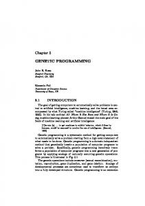
Fig. 1. function
Example of an AGP individual representing a multi-attribute
ber of pairs labeled during the training phase. The two proposed systems, named Alias and Active Atlas, respectively, obtain better results than the traditional approaches for data deduplication, which are usually based on supervised [18] or unsupervised [19] methods, while requiring minimal user intervention. Active Atlas was created to deal with data coming from different Web sources. Experimental results show that the active learning reduced the number of labeled trained data in two orders of magnitude, without losing any quality in the results. The system uses a committee of decision trees, in which pairs that generate maximum disagreement are sent to the user to label. Alias follows these same principles, but was conceived as a pure data deduplication tool. The results obtained by these methods encourage the development of semi-supervised approaches, as the one presented here. IV. ACTIVE L EARNING GP As most of the traditional deduplication methods that use learning for identifying replicas, AGP also works in three phases: (1) Generates all possible pairs of candidate records for comparison, exhaustively or through blocking techniques. (2) Calculates a similarity metric between each pair based on their attributes. In this phase, each attribute is manually associated with a well-known distance metric according to its type (i.e., numerical, short or long string). Details about these metrics are given in Section V. (3) Uses the similarity of each pair to learn how to deduplicate. This section focuses on phase 3, where a semi-supervised approach based on genetic programming and active and reinforcement learning finds a committee (set) of multiattribute functions that classifies a pair as a duplicate or not. Note that, although we focus on the data deduplication problem, the method proposed here can be easily adapted to any other application domain where labeling examples is an important and expensive process. Next, Section IV-A shows the individual representation used by AGP and Section IVB gives a general overview of the system, which is then described in detail in Sections IV-C to IV-E. A. Individual In the problem of data deduplication, each individual represents a similarity function between records. The trees that represent the similarity functions are generated using the four basic mathematical operators. The terminals are random
3 4 5 6 7 8 9 10 11 12 13 14 15 16 17 18
/* Preprocessing Generate a set of pairs P = p1 . . . pn from DB; Compute sim(p) for each pair p ∈ P ; R ← rank P according to sim(p) values ; Let T be the top k pairs in R ; Let B be the bottom k pairs in R ; User labels each pair p ∈ T ∪ B with Lp ∈ {T, F} ; Compute a weight WP for each p ∈ P ; /* Evolution Process Gen0 ← Generate m functions ; Evaluate(Gen0 ,T ∪ B); Compute a weight Wf for each function f ∈ Gen0 ; Com0 ← ∅; for i = 0 to a predefined number of generations do Comi ← top C functions in Geni ; /* Active Learning foreach pair p ∈ P do Comi labels p with Lp ∈ {T, F, D} ; if Lp = D then User labels p with L′ p ∈ {T, F} /*
Reinforcement
19 Update WP for each p ∈ P ; 20 Geni+1 ← Crossover&Mutation(Geni − Comi ); 21 Geni+1 ← Geni+1 ∪ Comi ; 22 Evaluate(Geni+1 , P ); 23 Compute Wf for each function f ∈ Geni+1 ; 24 Comi ← top C functions in Geni ; 25 foreach pair p ∈ P do 26 Comi labels p with Lp ∈ {T, F }
*/
*/
*/
*/
integers from 1 to 9, and the values of similarity between each attribute present in the database. Fig. 1 shows an example of a similarity function. The expression can be extracted by the tree in an infix manner. The tree in Fig. 1 represents the expression Reg Leven + (Reg tf idf /3) + Y ear IntM , where Reg Leven, Reg tf idf , and Y ear Intm represent the similarities between the register using the Leveinstein and tfidf measures, and the year using the IntMatch [2] measure, respectively. B. Process Overview Alg. 1 summarizes the AGP method proposed here to learn multi-attribute functions that classify pairs of records as duplicates or not. Initially, a Preprocessing step (Lines 3–9) generates a set P of pairs of records from a database DB being deduplicated. Typically, not all possible pairs from DB are in P since some blocking strategy might be used for pruning unlikely pairs. Next, a similarity function sim is deployed for estimating the similarity between records in each pair from P . This is a simple function that deploys predefined similarity functions for each attribute and sums the similarity values obtained. A rank R is then built over pairs p in P according to the values of sim(p). Finally, the algorithm takes T ⊂ P and B ⊂ P , which are respectively the top-k and the bottom-k pairs in R, and asks a user to label pairs in T and B as true (T) or false (F) pairs. The rationale behind this approach is to show to the user some pairs that are certainly duplicates (and hence are very similar, and are at the top of the ranking) and others that are certainly not (and are at
the bottom of the ranking). We notice in our experiments that T ∪ B corresponds to less than 1% of the pairs in the dataset. The preprocessing step ends in Line 9, in which a pair weight Wp is associated to each p ∈ P . This weight will be used throughout the process to indicate the confidence in the evaluation of a pair of records as duplicates or not, where the evaluation can be done by a user or a committee of functions, as detailed later in this section. Thus, based on the user’s judgment, those pairs in T ∪ B labeled with T receive Wp = 1 and those labeled with F receive Wp = −1. These values correspond to the maximum confidence for duplicates and non-duplicates, respectively. All others pairs in P receive Wp = 0. As the process goes on, these weights will move towards one of the maximum values. In Line 10, a set of individuals (record similarity functions) is generated, which corresponds to the first generation (Gen0 ) of the GP evolution. These functions undergo an evaluation process using only the labeled examples in T ∪B, i.e., they are used to classify them as duplicates or not according to a pre-defined threshold set as a percentage of the function maximum value (Line 12). Each individual in the population is associated with a function weight Wf (Line 12), which is proportional to how correctly each function evaluated the pairs in T ∪ B. This weight plays an important role in AGP since it is used as a fitness function. Subsequent generations are evolved on the Loop 14–23. In Line 15, a committee of functions is generate by taking the C functions from the current generation (Geni ) with highest Wf . The role of the committee in our approach is to choose which record pairs will be presented to the user to be labeled at each AGP generation. At this point (Lines 16–18), the committee is used to classify all examples in the dataset (labeled or not), where a majority voting process decides the pairs of labels (see Section IV-D for details on the active learning phase). In the case of a disagreement (Lp = D) that results from a tie, the user is called to classify the example. This step is followed by a reinforcement learning phase, implemented to exploit the relationships between the functions and the pairs they correctly classify. First, pair weights (Wp ) are updated to reflect the evaluation performed in Lines 16–18. For user-labeled pairs, weights are assigned as explained before (Line 9). For pairs labeled by the committee, weights are assigned based on the voting of the functions in the committee, also considering the weights of these functions (Wf ). In Lines 20 and 21, a new generation of functions (Geni+1 ) is created. While functions in the current committee are simply passed by elitism to this new generation (Line 21), the remaining functions undergo crossover and mutation operations (Line 20). As before, newly evolved functions evaluate pairs in P (Line 22). This time, however, function weights Wf are assigned based on how correctly each function evaluated the whole set of pairs P , considering the pair weights Wp . The reinforcement learning strategy we use involves the computation of Wf and Wp and is detailed in Section IV-E.
P1 P2 P3
F1 T T T
F2 F T T
Fig. 2.
F3 F T F
F4 F F F
Committee F T D
User T
The voting process
The evolution process stops when a maximum number of generations is reached. In this case, a new committee is created (Line 24) for labeling all pairs (Lines 25 and 26). Algorithm 2: EvaluateF(Generationi , Committei , Pairs) 1 foreach f in Generationi but not in Committei do 2 foreach p in Pairs do 3 Mp ← label(f,p) ; 4 switch (Lp , Mp ) do 5 case (+,+): Wf ← Wf + Wp ; 6 case (−,+): Wf ← Wf − Wp ;
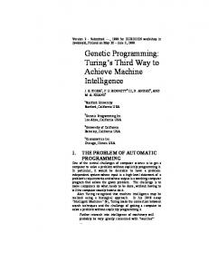
C. Evaluation of the Functions As previously explained, each individual in AGP represents a function used to classify the data pairs as duplicates or not. The fitness of each function is defined by a weight Wf and is a positive real number. The Wf of a function is defined according to the weights Wp of each record pair in the dataset. Recall that the values of the pair weights vary according to the classifications they receive from the committee. If the committee classifies a pair as duplicate (non-duplicate), the weight value of the pair is updated to be biased towards 1(-1). In the first generation (Line 12, Alg.1), Wf is set according to the value of the sum of the weights of the pairs (Wp ) correctly classified by the function as true, minus the sum of the weights of the labeled true pairs classified by the function as false. For this, labels assigned by the user to the pairs in T ∪ B are used as the ground truth. From the second generation until the last, function weights are computed similarly, with two differences: first, all pairs are considered; then the ground truth is taken either from the committee or from the user, when the committee disagrees (Line 23, Alg.1). Note that the weights of the functions that are members of the committee are not updated here, but during the reinforcement learning phase. Alg. 2 illustrates the process just described. As observed in lines 5-6, a function is only rewarded or penalized when classifying examples that are duplicates according to the user or the committee. D. Committee Voting and Active Learning The active learning process we deploy consists in using the committee to select which examples should be sent to the user to label. These examples are chosen according to the results of a voting process. The voting process is rather simple and based on the majority vote of the committee. Fig. 2 shows an example where four functions are used to classify three pairs. Note that, for pairs P 1 and P 2, the committee majority vote decides
the class of the example. Nevertheless, in P 3 there is a tie (disagreement) and the user is called to label the example. An important parameter of the system is the number C of members in the committee. In theory, the greater the number of individuals in the committee, the more they will disagree. This is true for the first generations, where the committees are very naive and tend to disagree in a high number of pairs. However, as the functions are evolved, the number of disagreements decrease and, consequently, the number of user interactions also decrease. Preliminary experiments showed that C is usually a small number. In the experiments reported here, for instance, the committee size was set to 20. However, to make sure the number of user interactions remain small, the method also works with a parameter that sets the maximum number of user interactions allowed per generation. Note that, during the voting process, we cannot guarantee that all the functions that are in the committee are good functions. Therefore, we want to associate a confidence to the committee vote. By itself, the committee does not have the authority to evaluate itself. Hence, the only way to do that is to compare its votes using a definitive source, such as the user labeled examples. In this way, votes of committee members that agree with the user have more value than the votes of those that only agree with the committee. Looking at Fig. 2, for instance, we can see that when classifying P 1 and P 2, F 2 and F 4 agree with the committee, and have the same confidence. However, when the user classifies P 3, only F 2 agrees with him/her. Hence, its confidence should be greater than the one in F 4. This shows the importance of the user in the learning process, and is considered during the reinforcement learning phase, described in the next section. E. Reinforcement Learning The idea of reinforcement learning introduced here was inspired on the HITS algorithm [20], used to calculate webpages relevance. In [20], a graph describes the relationships between a set of relevant authoritative pages and a set of hub pages. In the same way, here we describe the relationships between the functions in the committee and the pairs they correctly classify as duplicates. Given the pair weights and the function weights, in the reinforcement learning phase we assume that good functions are those that identify duplicates (giving them more weight), and that duplicates tend to be correctly identified by good functions. Hence, after each voting process, the pair weights are updated, followed by the function weights. The pair weight update method takes into account the result of the voting process. If in the previous voting a pair was labeled by the user, its weight is set to -1 (if non-duplicate) or 1 (if duplicate). Otherwise, it is updated according to C C ∑ ∑ Wf (T ) −
Wp = i=1
Wf (F ) i=1
where Wf (T) and Wf (F) are the function weights of the committee members that classified the pairs as duplicates
TABLE I F EATURES OF THE THREE DATASETS USED IN THE EXPERIMENTS Pesqsint Alias Restaurant Records 1000 254 864 Pairs 499,500 32,131 372,816 Duplicated Pairs 361 169 112 Attributes 6 6 5 Similarity Thresh. 0.7 0.5 0.8
or not, respectively. This value is normalized in the interval [-1,1]. The function weight of the committee members, in contrast, is given by the sum of the weights of the pairs (wp ) classified as true by the member minus the sum of the wp of the pairs classified as false by the committee member but as true by the final committee vote. When calculating the function weights, if the pair being considered is labeled, its weight is multiplied by a constant, which will reward or penalize the member for correctly (or incorrectly) classifying the pair. V. E XPERIMENTS This section reports the experiments run to test AGP, and is divided in four main parts. Section V-A describes the three datasets used to test the system, and Section V-B explains how the AGP parameters were chosen. Sections V-C and VD report the results obtained when comparing AGP with two other methods previously proposed in the literature, the GPbased method proposed in [12] (hereafter referred as GP) and ALIAS [2] (see Section III for more details), respectively. A. Datasets Experiments were performed with three datasets usually used for assessing data deduplication methods, namely Pesqsint, Alias, and Restaurant. Table I summarizes the main characteristics of these datasets. Note that, for each field in each dataset, we have to associate it with a similarity measure, which is used to calculate the distance between two pairs of records, determining if they are duplicates or not. Also, for each dataset, we need a similarity threshold, which decides if a pair is a duplicate or not according to the similarity function found by the GP. Pesqsint [12] is a synthetic dataset containing researchers’ personal data, and was created using the Data Set Generator Program (DSGP) available in Febrl [21]. This dataset has six fields, which were associated with the following similarity measures: NYSIIS for given name, DMetaphone for surnames, Jaro-Winkler for addresses, character-wise field comparison with a maximum number of errors (different characters) tolerance for locality names, geographical distance for postcodes, and age difference with error tolerance for age. Alias [2] is a collection of scientific articles extracted from Citeseer. Its six fields are associated with up to four different similarity measures, as follows: String-abrev, Levenstein and Jaccard for authors, Levenstein, Jaccard, SAME-TIT and tfidf for title, Intmatch for year, SAME-PAG and Keydiff for page, n-gram and Jaro-Winkler for author-title, and n-gram, Levenstein, Jaccard and tf-idf for record.
0.9
0.8
F−measure
Finally, Restaurant [17] contains data about American restaurants, including name, address, number, city and type. The following similarity measures were associated with each attribute: Jaro-Winkler and NAME-JWC with name, Soft tfidf and n-gram with address, Levenstein with city, Jaccard with number, and n-gram with type. The definitions and implementations of all these measures can be found in [12].
0.7
B. Genetic Programming Parameters The results reported in this paper use parameter configurations defined empirically during preliminary experiments. The only parameter for which we show its variations are shown is the number of generations. This is because the number of user interactions per generation and how it reflects on the accuracy of the system is crucial. Except for this variation, we run both AGP and GP with 80 individuals, and crossover and mutation rates of 0.98 and 0.02, respectively. For AGP, two extra parameters were necessary: the committee size and the maximum number of questions the committee could ask the user per generation. The former was set to 20 and the latter was set to 1 or 100, as explained next. According to the number of questions the committee could ask to the user, AGP can run in two different modes: committee-driven and generation-driven. The committeedriven mode is the one described in Section IV, where the committee is allowed to ask the user as many question as it finds necessary, as long as they do not exceed a maximum limit of questions. This is the way AGP is run when compared to the GP proposed in [12]. The generationdriven mode, in contrast, restricts the number of questions to one per generation. This restriction was imposed to allow a proper comparison between AGP and ALIAS. The reason for it is that, in the original version of ALIAS, the user is allowed to label exactly one pair of examples per round of active learning. C. AGP versus GP This section shows the results obtained when comparing the AGP system run in the committee-driven mode with the GP [12]. All the results reported from now on are an average over 20 genetic programming runs and were evaluated according to the quality of the deduplication (given by the F-measure) as well as the number of labeled examples the methods needed to find a good function. Recall that the F-measure is the weighted harmonic mean of precision and recall, and is given by F −measure =
2 × precision × recall . precision + recall
Precision is given by the number of duplicated pairs correctly identified divided by the number of pairs identified as duplicates. Recall is given by the number of pairs identified as duplicates over the total number of existing duplicated pairs. Before we present our results, it is important to emphasize that the GP obtained results are comparable to those obtained by state of the art deduplication algorithms. However, recall that GP follows a supervised approach, i.e. all the examples
0.6
Alias−AGP Pesqsint−AGP Restaurant−AGP Alias−GP Pesqsint−GP Restaurant−GP
0.5 1
2
3
Fig. 3.
4
5
6
Generation
7
8
9
10
11
12
Comparing the AGP with GP
used during the training process have to be labeled. AGP, in contrast, depends on the user to provide this information. In the preliminary experiments we run to compare AGP with GP, we trained the GP with all the available training data. Hence, for the dataset Pesqsint, for instance, all the 499,500 available pairs were used by GP to create a deduplication function. In the case of AGP, it initially had access to only two pairs previously labeled by the user. This number of available pairs increased as the evolutionary process went on and new pairs were labeled by the user during the active learning process without any restrictions. In these first experiments, both algorithms showed to be competitive in terms of deduplication quality. However, an analysis of the number of pairs labeled by the user during the AGP learning showed that this number was much smaller than the total number of labeled pairs available to GP. Taking into account that labeling pairs is a very expensive procedure, in a second experiment we reduced the number of pairs given to GP, so that it could use a maximum number of 100 pairs per generation (the same number of pairs an AGP user is allowed to label). The motivation for it was to find out if GP could also work with fewer examples while maintaining the quality of the deduplication. The results obtained by the AGP and GP regarding f-measure and the number of labeled pairs are presented in Fig. 3 and Table II. Fig. 3 shows the results of F-measure obtained by the best committee evolved by AGP (average over 20 runs) and the best individual evolved by GP when varying their number of generations from 1 to 10 (being the initial population considered as population 0). Note that usually GPs are left to evolve for many generations. However, preliminary experiments showed that, for the deduplication problem, both GP and AGP find very good individuals or committees with only few generations. According to a two-tailed paired t-test, the results obtained by AGP are statistically better than the results obtained by GP for Pesqsint and Restaurant with 99% confidence, and equivalent to those obtained by GP for Alias. Observe also that AGP finds a good solution to the problem in less generations than GP for Pesqsint and Restaurant. Table II shows the number of examples used by GP and
TABLE II R ESULTS OBTAINED
WHEN COMPARING THE
1.0
AGP
WITH THE
GP
IN
0.9 0.8
TERMS OF NUMBER OF LABELED EXAMPLES
Generations 0 1 2 3 4 5 6 7 8 9 10
GP 100 200 300 400 500 600 700 800 900 1000 1100
F−measure Alias
0.7
# of Labeled Examples PESQSINT Alias Restaurant 2 2 2 115.15 74 100.65 128.75 99.9 103.65 132.95 120.55 114.65 141.55 128.2 123.95 148.3 141.9 125.95 151.95 148.25 126.6 159.6 153.2 126.95 162.6 158.7 127.9 166.5 162.25 128.25 169.9 165.85 128.25
0.6 0.5 0.4 0.3 0.2 AGP Alias
0.1
0
10
20
30
40
50
60
70
80
90
100
Rounds of Active Learning
(a) Alias dataset
0.9
Committee Members (REG TFIDF*3)+REG LEVEN AT NGRAM+REG LEVEN+REG LEVEN (REG TFIDF/3)*PAG IGUAL REG NGRAM*ANO INTM 2-REG LEVEN+AT NGRAM REG LEVEN*ANO INTM ANO INTM*(REG LEVEN+REG LEVEN) REG LEVEN*ANO INTM ANO INTM*REG LEVEN REG LEVEN*ANO INTM AT NGRAM*ANO INTM REG LEVEN+AT NGRAM AT NGRAM+(REG TFIDF/3)+REG LEVEN REG LEVEN+REG LEVEN+REG TFIDF AT NGRAM+REG LEVEN AT NGRAM+REG TFIDF AT NGRAM+REG LEVEN REG TFIDF+AT NGRAM AT NGRAM+REG LEVEN REG TFIDF+REG NGRAM
Fig. 4.
F−measure Restaurant
0.8
0.7
0.6
AGP Alias
0.5
AGP Committee Members 0
10
20
30
40
50
60
Rounds of Active Learning
70
80
90
100
(b) Restaurant dataset 1.0
0.9
F−measure Pesqsint
AGP for executions with different numbers of generations. Note that, for GP, the number of available examples increases by 100 at each generation. For the AGP, in contrast, two examples are given in generation 0 and, from there on, a maximum number of 100 examples can be labeled per generation. Observe, however, that from these 100 available examples, the number of actually labeled ones will vary according to the number of calls made to the user to untie a committee voting process. Table II shows that, in the worst case scenario, AGP labeled around 170 examples out of the 1100 permitted (100 examples × 11 generations) for the dataset Pesqsint. In this same run, GP relied on the 1100 examples. In sum, Table II shows that AGP will never need as many labeled examples as the ones available for GP. The experiments also showed that, as evolution goes on, a smaller number of calls to the user is made and this number becomes stable after a few generations. From all the runs performed by AGP and GP, we selected to report here the best committee found by AGP, as showed in Fig. 4, and the best individual found by GP for the dataset Alias. The AGP committee in Fig. 4 obtained an Fmeasure of 0.973 and used only 211 labeled examples. The best deduplication function found by GP, in contrast, was REG LEV EN + REG JACC + AT N GRAM , with an F-measure of 0.913 and 1100 labeled examples. While the GP function uses three different attributes in the evolved function, all together the 20 functions of the committee involve seven different attributes. Note that attribute REG JACC, used by GP, does not appear in the AGP committee. Also observe the current version of AGP allows the committee to have one or more copies of a good individual. This is equivalent to adding more weight to a vote of a very good individual. However, further studies on this matter are left for future work. Finally, when we compare AGP and GP in terms of perfor-
0.8
0.7
0.6
0.5 AGP Alias
0.4
0.3 0
10
20
30
40
50
60
Rounds of Active Learning
70
80
90
100
(c) Pesqsint dataset Fig. 5.
Comparing AGP and Alias with 100 active learning rounds
mance, we observe that AGP is slower than GP. The reason for that is AGP uses all the unlabeled examples while evaluating the evolved functions, while GP uses only the labeled pairs (which, in our experiments, correspond to a maximum of 10% of the total dataset). For this reason, GP runs for the dataset Pesqsint in 0.125 seconds, while AGP runs in 56.26 seconds. However, this problem can be easily solved by using some blocking technique to discard the pairs that are certainly not duplicates, or adding a transductive learning approach to the current method, as explained in Section VI. D. AGP versus ALIAS This section presents the results obtained when comparing the proposed AGP with ALIAS. This comparison is interesting as ALIAS uses an active learning procedure to select the instances that will be labeled by the user, but instead of using a genetic programming algorithm to learn a multi-attribute function, it uses either a decision tree, a Naive Bayes or an SVM algorithm. In the experiments showed in this section, AGP is compared with ALIAS using
decision trees, once in [2] the authors showed this method finds the best F-measure overall. The experiments reported here followed the generationdriven approach. This is because ALIAS works with the concept of active learning round, where one pair is labeled per round and the total number of learning rounds corresponds to the total number of labeled pairs. Hence, each round of active learning corresponds to a generation of AGP where one labeled example was made available to the system. Fig. 5 shows the graphs for the three datasets of the number of active learning rounds (x-axis) against the F-measure(y-axis). The graphs show that, for the three datasets, the AGP curve dominates the ALIAS curve. We can also observe that the learning process of AGP is much faster than the learning process of ALIAS, as the first solutions found by AGP are much better than those found by ALIAS (apart from the first ones found for the dataset Restaurant) and, as more rounds are executed, the AGP curve becomes stable much faster than the ALIAS curve. Although AGP has lower F-measure than ALIAS in the first round for the dataset Restaurant, the graph shows us that, after the first round, ALIAS loses all its stability, improving or degrading its F-measure until it reaches active learning round 45. At the end of the 100 active learning rounds, AGP obtains statistically significant better results than those obtained by ALIAS according to a paired t-test with 99% confidence. For the Alias dataset, which was the one in which ALIAS was originally tested, AGP best and worst F-measures are 96.8% and 36.6%, while for ALIAS they are 94.7% and 0%. More importantly, the AGP curve is more stable, with the F-measure dropping in only few situations. The ALIAS curve, in contrast, can drop significantly after new labeled examples are added to the training set (as observed in rounds 59 and 60). VI. C ONCLUSIONS AND F UTURE W ORK This paper introduced an active learning genetic programming algorithm, named AGP, and instantiated it for the task of record deduplication. The method follows a semi-supervised approach and uses the principles of active and reinforcement learning to evolve a committee of multiattribute functions. The system requires the assistance of an user when the committee members do not reach a decision of whether the record pair represents a duplicate or not. At the end of the evolution process, the best committee is used to identify replicas. The proposed method was tested in three datasets and compared to two other deduplication methods previously proposed in the literature, namely the supervised genetic programming method proposed in [12] and the semi-supervised active learning method proposed in [2]. The results show that the quality of the deduplication produced by AGP is as high as the quality of the results obtained by the other two methods. However, AGP needs less user intervention during the training process and is stable and consistent. As future work, we intend to add to AGP some transductive learning principles, so that examples classified by the
committee with a confidence higher than a threshold can be automatically considered as ground truth and excluded from the unlabeled training set. This modification would reduce the runtime of AGP, as fewer examples would have to be evaluated by the evolved functions at each generation. The application of AGP to other classification problems in which labeling data is expensive, such as text classification, will also be studied. ACKNOWLEDGMENT This work was partially supported by CAPES, CNPq, FAPEMIG, Santander, and INWeb. R EFERENCES [1] W. Banzhaf, P. Nordin, R. Keller, and F. Francone, GP – An Introduction; On the Automatic Evolution of Computer Programs and its Applications. Morgan Kaufmann, Jan. 1998. [2] S. Sarawagi and A. Bhamidipaty, “Interactive deduplication using active learning,” in Proc. of the 8th ACM SIGKDD, 2002, pp. 269–278. [3] O. Chapelle, A. Zien, and B. Sch¨olkopf, Semi-supervised learning. MIT Press, 2006. [4] C. Rosenberg, M. Hebert, and H. Schneiderman, “Semi-supervised self-training of object detection models,” in Proc. of the 7th IEEE Workshop on Application of Computer Vision, 2005, pp. 29–36. [5] A. Blum and T. Mitchell, “Combining labeled and unlabeled data with co-training,” in Proc. of the 11th Annual Conf. on Computational Learning Theory, 1998, pp. 92–100. [6] Y. Hong, S. Kwong, H. Xiong, and Q. Ren, “Genetic-guided semisupervised clustering algorithm with instance-level constraints,” in GECCO ’08: Proceedings of the 10th Annual Conf. on Genetic and Evolutionary Computation, 2008, pp. 1381–1388. [7] D. A. Cohn, L. Atlas, and R. Ladner, “Improving generalization with active learning,” Mach. Learning, vol. 15, no. 2, pp. 201–221, 1994. [8] A. Beygelzimer, S. Dasgupta, and J. Langford, “Importance weighted active learning,” in ICML ’09: Proc. of the 26th Annual Int. Conf. on Machine Learning. New York, NY, USA: ACM, 2009, pp. 49–56. [9] C. R., L. P., and H. M.I., “Scaling genetic programming to large datasets using hierarchical dynamic subset selection,” IEEE Trans Syst Man Cybern B Cybern., vol. 37, no. 4, pp. 1065–1073, 2007. [10] C. Gathercole and P. Ross, “Dynamic training subset selection for supervised learning in genetic programming,” in Proc. of the Int. Conf. on Evolutionary Computation, London, UK, 1994, pp. 312–321. [11] L. Jin, C. Li, and S. Mehrotra, “Efficient record linkage in large data sets,” in Proc. of the 8th Int. Conf. on Database Systems for Advanced Applications, 2003, pp. 137–148. [12] M. G. de Carvalho, M. A. Gonc¸alves, A. H. F. Laender, and A. S. da Silva, “Learning to deduplicate,” in Proc. of the 6th ACM/IEEE-CS Joint Conference on Digital Libraries, 2006, pp. 41–50. [13] M. G. Carvalho, A. H. F. Laender, M. A. Gonc¸alves, and A. S. da Silva, “Replica identification using genetic programming,” in Proc. of the ACM Symposium on Applied computing, 2008, pp. 1801–1806. [14] A. A. Freitas, Data Mining and Knowledge Discovery with Evolutionary Algorithms. Springer-Verlag, 2002. [15] M. Bilenko, “Learnable similarity functions and their application to record linkage and clustering,” Ph.D. dissertation, University of Texas at Austin, 2006. [16] C. W. G. Lasarczyk, P. W. G. Dittrich, and W. W. G. Banzhaf, “Dynamic subset selection based on a fitness case topology,” Evol. Comput., vol. 12, no. 2, pp. 223–242, 2004. [17] S. Tejada, C. A. Knoblock, and S. Minton, “Learning domainindependent string transformation weights for high accuracy object identification,” in Proc. of the 8th ACM SIGKDD, 2002, pp. 350–359. [18] M. Bilenko and R. J. Mooney, “Adaptive duplicate detection using learnable string similarity measures,” in Proc. of the 9th Int. Conf. on Knowledge Discovery and Data Mining, 2003, pp. 39–48. [19] L. Gu and R. Baxter, “Decision models for record linkage,” in Data Mining, 2006, pp. 146–160. [20] J. M. Kleinberg, “Authoritative sources in a hyperlinked environment,” J. ACM, vol. 46, no. 5, pp. 604–632, 1999. [21] T. F. Christen, P.; Churches, Febrl Freely extensible biomedical record linkage, http://sourceforge.net/projects/febrl.