topic is a good strategy in selecting the data to label, con- sidering that labeling data is ... a supervised learning algorithm to train a classifier on . The selection engine ..... ent proportions between the numbers of face and non-face images in the ...
Active Learning Using Pre-clustering
Hieu T. Nguyen TAT @ SCIENCE . UVA . NL Arnold Smeulders SMEULDERS @ SCIENCE . UVA . NL Intelligent Sensory Information Systems, University of Amsterdam, Faculty of Science, Kruislaan 403, NL-1098 SJ, Amsterdam, The Netherlands
Abstract The paper is concerned with two-class active learning. While the common approach for collecting data in active learning is to select samples close to the classification boundary, better performance can be achieved by taking into account the prior data distribution. The main contribution of the paper is a formal framework that incorporates clustering into active learning. The algorithm first constructs a classifier on the set of the cluster representatives, and then propagates the classification decision to the other samples via a local noise model. The proposed model allows to select the most representative samples as well as to avoid repeatedly labeling samples in the same cluster. During the active learning process, the clustering is adjusted using the coarse-to-fine strategy in order to balance between the advantage of large clusters and the accuracy of the data representation. The results of experiments in image databases show a better performance of our algorithm compared to the current methods.
1. Introduction In recent years, research interest has been attracted to semisupervised learning or learning in the condition that only a small initial amount of data is labeled while the majority of the data remain unlabeled. While many methods focus to improve the supervised learning by using the information from unlabeled data (Seeger, 2001), another important topic is a good strategy in selecting the data to label, considering that labeling data is a time-consuming job. The topic is known as active learning (Lewis & Gale, 1994). Consider the problem of learning a binary classifier on a � ���� � � � ���� � . Let partially labeled database
��
Appearing in Proceedings of the International Conference on Machine Learning, Banff, Canada, 2004. Copyright 2004 by the first author.
� be the labeled set in which every sample is given a la�� � � � � �. The active learning bel � � � � �, and
system comprises two parts: a learning engine and a selection engine. At every iteration the learning engine uses � a supervised learning algorithm to train a classifier on . � The selection engine then selects a sample from and requests a human expert to label the sample before passing it to the learning engine. The major goal is to achieve a good classifier as best as possible within a reasonable number of calls for labeling by human help.
Current methods on active learning can be characterized by their base learning algorithms which include probabilistic naive Bayes (Nigam et al., 2000; Roy & McCallum, 2001), combination of naive Bayes and logistic regression (Lewis & Gale, 1994), and the Support Vector Machine (SVM) (Campbell et al., 2000; Tong & Koller, 2001; Schohn & Cohn, 2000). The naive Bayes classifier suffers from two problems. First, the classifier assumes the independence between the component features of �. This assumption is often violated. The second problem is that naive Bayes is a generative model for which training relies on the estimation of the likelihood ������. This estimation is inaccurate in the case of active learning since the training data are not randomly collected. The paper focuses on discriminative models including logistic regression and SVM. These models aim to estimate the posterior probability ��� ���. They are less sensitive to the way the training data is collected, and hence, are more suitable for active learning. A more theoretical consideration is given in (Zhang & Oles, 2000). It is crucial to choose the most “valuable” training samples. Many methods choose the most uncertain samples which are closest to the current classification boundary. We name this approach the closest-to-boundary criterion. This simple and intuitive criterion performs well in some applications (Lewis & Gale, 1994; Tong & Chang, 2001; Schohn & Cohn, 2000; Campbell et al., 2000). Some other criteria have been proposed specifically for SVM. In (Campbell et al., 2000), it is proposed to select the sample that yields the largest decrease of the margin between the two classes. The method of (Tong & Koller, 2001) selects the
sample that halves the permitted region of the SVM parameters in the parameter space. Both (Campbell et al., 2000) and (Tong & Koller, 2001) need to predict the values of the SVM parameters for every possible case where a candidate sample might be added to the training set. Since it is hard to do this efficiently, the references finally resort to the closest-to-boundary criterion. The closest-to-boundary methods ignore the prior data distribution which can be useful for active learning. In (Cohn et al., 1996), it is suggested to select samples that minimize the expected future classification error:
�� � ������ ��� ������ � �� � (1) �� � where ���� is� the true label of � and �� � �� is the classifier ��� output. � � denotes the expectation over ��� ���. Due to
the complexity of the integral, the direct implementation of eq. (1) is usually difficult. However, it shows that the data uncertainty should be weighted with the prior density ����. If ���� is uniform or unknown, the expectation under the integral is the contribution by a sample into the classification error. The expectation can then be used to measure the value of the sample in the condition that the computation of the integral is complex. Under the assumption that the current classification boundary is good, it is easy to show that the error expectation is maximal for the samples lying on the classification boundary, see section 3.3. When ���� is known and non-uniform, the information about the distribution can be used to select better data. In this paper ���� is obtained via clustering which can be done offline without the interaction with human. The clustering information is then useful for active learning in two ways. First, the representative samples located in center of clusters are more important than the other, and should be selected first in labeling. Secondly, samples in the same cluster are likely to have the same label, (Seeger, 2001; Chapelle et al., 2002). This assumption should be used to accelerate active learning by reducing the number of labeling samples from the same cluster. The idea to combine clustering and active learning has appeared in previous work. In (McCallum & Nigam, 1998), a naive Bayes classifier is trained over both labeled and unlabeled data using an EM algorithm. Under the condition that the overwhelming majority of the data is unlabeled, that training algorithm amounts to clustering the data set, and the role of the labeled data is for initialization only. Clustering information also contributes to the selection where an uncertainty measure is weighted with the density of the sample. The referenced approach does not match, however, the objective of this paper to combine clustering with a discriminative model. Several other active learning schemes also weigh the uncertainty with the data density (Zhang & Chen, 2002; Tang et al., 2002). Some
methods put more emphasis on the sample representativeness by selecting cluster centers from a set of most interesting samples. In the representative sampling by (Xu et al., 2003), the algorithm uses the k-means algorithm to cluster the samples lying within the margin of a SVM classifier trained on the current labeled set. The samples at cluster centers are then selected for human labeling. The method of (Shen & Zhai, 2003) has a similar idea, but applies the kmedoid algorithm for the top relevant samples. In general, heuristic methods have been proposed to balance between the uncertainty and the representativeness of the selected sample. They encourage the selection of cluster centers. However, no measure has been taken to avoid repeatedly labeling samples in same cluster. In addition, there are important questions that remain open, namely, how to adapt the classification model for a training set that contains only cluster centers? and, how to classify samples that are disputed by several clusters? This paper presents a solution for these issues using a mathematical model that explicitly takes clustering into account. The organization of the paper is as follows. Section 2 describes the incorporation of the clustering information into the data model, and provides the theoretical framework for the data classification. Section 3 presents our active learning algorithm. Section 4 shows the results of the algorithm for the classification of images in test databases.
2. Probabilistic framework 2.1. Data model In the standard classification, data generation is described by the joint distribution ���� �� of the data � and the class � � � label � � � � �. The clustering information is explicitly incorporated by introducing the hidden cluster la�� bel � � � � �� � �, where � is the number of clusters in the data. indicates that the sample belongs to the -th cluster. Assume that all information about the class label � is already encoded in the cluster label . This implies that once is known, � and � are independent. The joint distribution is written as:
���� � � � � ��� ��� ����� ��� � � ��� � ����� ��� �
(2) The simple Bayesian belief net representing the model is cluster label k y class label
x data
Figure 1. The Bayesian net for the data model.
depicted in Figure 1.
Before giving the specific form for the three distributions in eq. (2) we remark that a similar scheme has been proposed for the passive semi-supervised learning (Miller & Uyar, 1996; Seeger, 2001). The conceptual difference, however, between their approach and ours is in the definition of ��� � �. In the references, ��� � � is defined within individual clusters. As a consequence, the estimation of the parameters of ��� � � can be unreliable due to insufficient labeled data in a cluster. In our model, ��� � � is defined for all clusters with the same parameters. We use logistic regression for ��� � �:
��� � � � �
� � �� ����� �� ���
(3)
Here, �� is a representative of the -th cluster which is determined via clustering. � � � and � � � are the logistic regression parameters. In essence, ��� � � is the label model for a representative subset of the database. In the ideal case where data is well clustered, once all the parameters of ��� � � are determined, one could use this probability to determine the label of the cluster representatives, and then assign the same label to the remaining samples in the cluster. In practice, however, clustering can be inaccurate and we will have problems with classification of samples at border between the clusters. To achieve better classification for those samples, we use a soft cluster membership which allows a sample to be connected to more than one clusters (representatives) with a probability. The noise distribution ���� � is then used to propagate information of label � from the representatives into the remaining majority of the data, see Figure 2. We use the isotropic Gaussian model:
� ���� � � �� � �� �
��
�� � � � � � �� � �
(4)
�
where is the variance assumed to be the same for all clusters. representatives classifier for the representatives +
+
�
In the presented method, the parameters ��, �, ��and � are estimated from the data. The scale parameter is given initially. It can be changed during active learning when a different clustering setting is needed. 2.2. Data classification
Given the above model, one calculates ��� ���, the posterior probability of label of a sample as follows: � � ��� ��� � ���� ��� � ��� � ���� ��� � ��� ���
where �� ���
(5)
� ���� ��� ������.
Data are then classified using the Bayes decision rule:
� � �� �� � �� �
� ���� ��� ��� � ��� � ����� ��� ���
if ��� otherwise
(6) � � �� denote the current estimates of the parameters. where � Observe from eq. (5) that the classification decision is a weighted combination of the classification decision for the representatives. Well clustered samples will be assigned the same label as the nearest representative. Samples disputed by several clusters, on the other hand, will be assigned the label of the cluster, which has the highest confidence. Note that the weights �� ��� are fixed unless the data are re-clustered whereas ��� � � is updated upon the arrival of new training data.
3. Description of algorithm The parameters of the model proposed in section 2.1 are estimated via likelihood maximization. The data likelihood comprises two parts: the likelihood of the labeled data and the likelihood of the unlabeled data: �
�
� � ���� � �� � � ���� � ���� �� ���� ��
(7)
�
where � and � denote the set of indices of labeled and unlabeled samples respectively. Expanding ���� � �� � as �� the sum of ���� � and ���� ��� �, the likelihood (7) can �� �� be written with explicit dependence on the parameters as follows:
� � � � � ��� � � � � � � �� �� � � �� �� � �� � ��� �� � � � � � ��� � � � � � � �� � � ������� ��
� �
−
actual classifier
�
Figure 2. The classification model
� ��. Then, ���� is a mixture of � Gaussians Let �� � � with the weights �.
���� ��
���� ��� � ��� � � � � �� � �� ��
(8)
As the amount of the unlabeled data is overwhelming over the labeled data, the parameters ��� � � � � � and �
�
�� � � � � �
are determined mainly by maximizing the first term in eq.� (8). The maximization of each term can therefore be done separately. The clustering algorithm maximizes the likelihood of the data samples to obtain the cluster representatives and the cluster prior. The maximization of the label likelihood follows to estimate the parameters � and �. data samples
������
������ �
� ��� � �� � �� � �� ��� �
(9)
where � � denotes the set of indices of the samples in the
-th cluster. The process of cluster fission is completed when: � � (10) �
�� � � �
�
���
where is a predefined constant. We have used . Thus, the cluster size and the final number of clusters � is controlled by the scale parameter .
Initial clustering (section 3.1)
Once the cluster representatives ��� � � � � � have been de� termined, the cluster prior � is obtained�by iterating the following two equations until stability:
���������
�� �� �� � �� � �� � � ���
� �� �� � � ���� �� ��� ���� ���� �� � ��� � �(11) � �� �� � ��� (12) � ��� �� �
Estimating p(y|k) (section 3.2)
Calculating p(y|x) eq. (5)
� � ������
STOP?
two smaller ones with:
YES
END
3.2. The estimation of the class label model NO
��� � � based on the maximization of the second likelihood � This section presents the estimation of the distribution
Selecting and labeling an unlabeled sample, eq. (30)
in eq. (8). Fixing the cluster representatives �, the likelihood depends only on the parameters � and �:
��� � ���� ��� � �� �� ��� ���� ��
Cluster adjustment (section 3.4)
������������
Figure 3. The proposed active learning algorithm.
The block scheme of the algorithm is illustrated in Figure 3. 3.1. Initial clustering In the presented algorithm, the goal of clustering is data representation rather than data classification. We therefore use the � -medoid algorithm of (Kaufman & Rousseeuw, 1990). The algorithm finds � representatives ��� � � � � � � of the data set ��� � � � ��� so as to minimize the sum of the distance from the data samples to the nearest representative. See (Struyf et al., 1997) for the detailed implementation. The � -medoid algorithm is computationally expensive when either or � is large. In practical applications both numbers are very large indeed. The following simplifications are employed to reduce computations. First, the data set is split into smaller subsets. The � -medoid algorithm is then applied to cluster every subset into a limited number � of clusters. Clustering is continued by subsequently breaking the cluster with the largest radius � into
�
�
�
(13)
From eq.(5), ���� ��� � �� �� can be written as a mixture of � logistic distributions ���� � � �� �� with the weights �� ��� �.
�
In case the dimensionality is higher than the number of the labeled samples, the optimization in (13) is numerically unstable. The conventional approach to the prob� overcome � lem is to add a regularization term � � where is a predefined parameter. This leads to the minimization of the following objective function:
�
� ��� �� � �� � � � � �
���� ��
�
�� �
��
��� � � � �� � � �� ���� �
(14) Remark that eq. (14) is the extension of the regularized logistic regression (Zhang & Oles, 2001; Zhu & Hastie, 2001) for the mixture of the logistic distributions.
�
The minimization of is implemented using Newton’s algorithm which guarantees to find a local minimum. Furthermore, since is convex, it has only one local minimum which is also the global minimum.
�
�
�
Starting with an initial guess � and � , the parameters � and � are updated iteratively. At each iteration, the param-
eter increment in the steepest direction is:
�� �� �
��
� �� ���
�
�
(15)
�
where is the Jacobian of , and is a positive definite approximation of the hessian matrix of . Using eq.(3), it can be shown that:
�� � ��� � �� �� �
��
�� �
�
� � � �� � �� �
�
�
�
� � ������ � � �� �� � � ���� � � �� ��� �� ��� � � ���� ��� � �� �� ����
(17) For the hessian matrix, the following approximation can be used:
�
where
�
�
��
� � � � � � �� � � � �� � ��
��
��
��
3.3. Criterion for data selection (16)
where �
only. As will be seen in the next subsection, the presented algorithm tends to select the training data from the cluster representatives. The number of non-zero � is then small,
approximately the same � �as the number of labeled samples. The computation of in eq. (25) can then be done effi ciently by suppressing the columns in which correspond to � that equal to zero.
(18)
The selection criterion gives priority to two types of samples: samples close to the classification boundary and samples which are cluster representatives. Furthermore, within the set of cluster representatives, one should start with the highest density clusters first. We have noted that the computation of the future classification error in eq.(1) is complicated. So, instead of choosing the sample that produces the smallest future error, we select the sample that has the largest contribution to the current error. Although such approach does not guarantee the smallest future error, there is a good chance for a large decrease of the error. The selection criterion is:
� � ��� ���
is the identity matrix and:
� ����
� ���� � � �� ��
� � ���� � � �� ��� �� ��� � � ���� ��� � �� �� (19)
To get more insight into eq.(15), let:
�
�
� �
� � � �� � � � � ��
��
� � � � � �
� � �
�
� �� � � � �
�
�
(20) (21) (22)
� ��
matrix whose columns are the vectors � � �� is the . One can show that:
�� �� �� � �� � � �� �
�� (23) � � � � � � � �� � � � � � �� � � � � � (24)
�� �� � � �
� � �
� � � �
��
��
using the Woodbury
�
�
� � � �
� ����
�
� �� �� ���� ���� �
(26)
where � denotes the index of the selected sample.
The error expectation for an unlabeled �� is calculated over the distribution ���� ��� �:
� �� �� ���� � � ���� � ���� ����� � �� ���� � ����� ����� �� � � � ���� ����� � ���� � � ���� � ����� �� (27) � ���� � is unIt should be noted that the probability ���� known and needs to be approximated. An obvious choice is � ���� � ��� ���, assuming to use the current estimation ���� � � � �� are good enough. Letting � �� � � � ���� � ���� � ��� ��� � ���� � ����� � ��� ��� (28) �� ����
�
Here,
If is high, it is efficient to invert formula:
����
(25)
it follows from eq. (5) that:
� ����
�
(29)
Observe that if ��� lies on the current classification boundary, the quantity � ��� � � is minimal, and hence the expected error is maximal. Eq. (26) becomes:
� � ��� ��� �� � �� ��� � ������ �
�
If all � are non-zero, the�size of is � � . Since �
is large, the inverting of as in eq. (25) would be computationally expensive still. However, remark that for a sample �� there are only few values of such that �� ��� � is different from zero, especially if �� is a cluster representative. In the latter case, the sample typically belongs to one cluster
� �� �� ���� � � �� � �� ��� � ��
����
where � ���� � � ���� ��
��
�� � �� �� � �� � �
(30)
(31)
�
�
(http://yann.lecun.com/exdb/mnist/). The size of images is � �� . The objective is to separate the images of a given digit against the other nine. In the experiments the following setting was used. The images are considered as the vectors composed of the pixel grey values which range from 0 to 255. The initial training set contains equal numbers of object and non-object � �� images. The initial size of this set was � and was in � � creased to during active learning, where is the number of samples in the database. For clustering, the databases were split into subsets per 1250 samples. The � -medoid algorithm was applied for each subset with the � ��. The initial value of initial number clusters � � � �of � �� was where is the number of pixels in one image. For the estimation of the class label distribution, we � �. use the regularization coefficient
�
�
Figure 4. Example view of images in the first database.
�
The resulting criterion indeed satisfies the demands� put in � the beginning of the subsection. The term � � � ��� � �� gives priority to the samples at the boundary. Meantime, ���� � gives priority to the representatives of dense clusters.
The labeling of high density clusters promises a substantial move of the classification boundary. It is therefore advantageous to group the data into large clusters in the initial clustering. This is achieved by setting a high value for the initial scale parameter . When the classification boundary reaches the border between the global clusters, a finer clustering with smaller cluster size is better to obtain a more accurate classification boundary. The maximum in eq. (30) can be used as the indication for the need to adjust the clustering. If this quantity drops below a threshold �:
�
����
�
(32)
the scale parameter is decreased:
��� �
� �
(33) � � where � � . The data set is then re-clustered. The � � � �� parameters � and are predefined. We have used � � � � �� and . Note that clustering the data set with different
�
�
� �
Every time a new training sample is added, the classifier is re-trained and tested on the rest of the database. The classification error is calculated as the sum of the missed positives and false alarms relative to . The performance evaluation is based on the decrease of the classification error as the function of the amount of training samples.
�
3.4. Coarse-to-fine adjustment of clustering
��� �� � �� ��� ������� � �
�
�
�
scales can be done offline. Furthermore, change of the scale takes place not in every iteration, but only few times during the learning process.
4. Experiments We have performed two experiments to test the performance of the proposed algorithm. In the first experiment, the algorithm is applied to find human face images in a �� � �� database containing 2500 images of size . See (Pham et al., 2002) for details on how the images were created. Example views of some images are shown in Figure 4. In the second experiment, a test database was made of images of handwritten digits taken from the MNIST database
For comparison, we have also implemented three other active learning algorithms. They use the standard linear SVM for classification. The first algorithm selects training data randomly. In the second algorithm, data are selected according to the closest-to-boundary criterion. The third algorithm uses the representative sampling of (Xu et al., 2003) which selects the medoid centers in the SVM margin. As we select one sample per iteration, this leads to selection of the most representative sample among the samples in the margin. Figure 5 shows the result of the first experiment for different proportions between the numbers of face and non-face images in the database. Figure 6 shows the result of the second experiment for the different sizes of the database. Both figures show the average of the classification error obtained by repeating the experiments with three different initial training sets that are picked up randomly. The results of Figure 6 are also an average over the ten digits. The proposed algorithm outperforms all three other algorithms. The most significant improvement is observed in Figure 5a with equal numbers for object and non-object samples in the database. The improvement decreases when the amount of the object samples is small relative to the non-object samples, see Figure 5c. In this case, since there are no clusters of the object class, the proposed algorithm is not advantageous over the closest-to-boundary algorithm in finding object samples. Nevertheless, the proposed algorithm remains better as it still benefits from the clustering of non-object samples. Representative sampling turns out
n1=1250, n2=1250
random sampling closest−to−boundary representative sampling proposed algorithm
0.18
0.14
0.12
0.1
0.08
0.06
0.16
0.14
0.12
0.1
0.08
0.06
0.14
0.12
0.1
0.08
0.06
0.04
0.04
0.04
0.02
0.02
0.02
0
0
a)
0.5
1
1.5
2
2.5
3
3.5
percentage of labeled data (%)
b)
0.5
1
1.5
2
2.5
3
3.5
percentage of labeled data (%)
0
c)
n=1250
0.1
0.08
0.06
0.16
0.14
0.12
0.1
0.08
0.06
0.12
0.1
0.08
0.06
0.04
0.02
0.02
0.02
0
0
2
2.5
3
3.5
b)
3.5
0.14
0.04
1.5
3
0.5
1
1.5
2
2.5
3
percentage of labeled data (%)
random sampling closest−to−boundary representative sampling proposed algorithm
0.18
0.04
percentage of labeled data (%)
2.5
n=5000
averaged classification error
averaged classification error
0.16
0.12
2
0.2
random sampling closest−to−boundary representative sampling proposed algorithm
0.18
0.14
1
1.5
percentage of labeled data (%)
0.2
random sampling closest−to−boundary representative sampling proposed algorithm
0.5
1
n=2500
0.2
0.16
0.5
� and � are the number of face and non-face images in the databases
Figure 5. The results for the classification of face images. respectively.
0.18
random sampling closest−to−boundary representative sampling proposed algorithm
0.18
averaged classification error
0.16
averaged classification error
averaged classification error
0.16
averaged classification error
0.2
0.2
random sampling closest−to−boundary representative sampling proposed algorithm
0.18
a)
n1=125, n2=2375
n1=500, n2=2000
0.2
0
3.5
c)
Figure 6. The classification results of handwritten digits from the MNIST database.
0.5
1
1.5
2
2.5
3
percentage of labeled data (%)
is the database size.
to perform better only than random sampling. A possible reason could be the undervaluation of the uncertainty and the lack of a proper classification model.
the main purpose of the paper is to show the advantage of using clustering information. We have succeeded in that goals for the given datasets.
5. Conclusion
References
The paper has proposed a formal model for incorporation of clustering into active learning. The model allows to select most representative training examples as well as to avoid repeatedly labeling samples in same cluster, leading to better performance than the current methods. To take the advantage of the similarity between the class label of data in the same cluster, the method first constructs a classifier over the population of the cluster representatives. We use regularized logistic regression which is a discriminative model with state-of-the-art performance and which is naturally fitted into a probabilistic framework. The gaussian noise model is then used to infer the class label for non-representative samples. New training data are selected from the samples having the maximal contribution to the current expected error. In addition to closeness to the classification boundary, the selection criterion gives priority also to the representatives of the dense clusters, making the training set statistically stable.
Campbell, C., Cristianini, N., & Smola, A. (2000). Query learning with large margin classifiers. Proc. 17th International Conf. on Machine Learning (pp. 111–118). Morgan Kaufmann, CA.
The method was restricted to linear logistic regression as
Chapelle, O., Weston, J., & Scholkopf, B. (2002). Cluster kernels for semi-supervised learning. Advances in Neural Information Processing Systems. Cohn, D. A., Ghahramani, Z., & Jordan, M. I. (1996). Active learning with statistical models. Journal of Artificial Intelligence research, 4, 129–145. Kaufman, L., & Rousseeuw, P. (1990). Finding groups in data: An introduction to cluster analysis. John Wiley & Sons. Lewis, D. D., & Gale, W. A. (1994). A sequential algorithm for training text classifiers. Proceedings of SIGIR94, 17th ACM International Conference on Research
3.5
and Development in Information Retrieval (pp. 3–12). Springer Verlag. McCallum, A. K., & Nigam, K. (1998). Employing EM in pool-based active learning for text classification. Proc. 15th International Conf. on Machine Learning (pp. 350– 358). Morgan Kaufmann, CA. Miller, D., & Uyar, H. (1996). A mixture of experts classifier with learning based on both labelled and unlabelled data. Advances in Neural Information Processing Systems 9 (pp. 571–577). Nigam, K., McCallum, A., Thrun, S., & Mitchell, T. (2000). Text classification from labeled and unlabeled documents using EM. Machine Learning, 39, 103–134. Pham, T., Worring, M., & Smeulders, A. (2002). Face detection by aggregated bayesian network classifiers. Pattern Recogn. Letters, 23, 451–461. Roy, N., & McCallum, A. (2001). Toward optimal active learning through sampling estimation of error reduction. Proc. 18th International Conf. on Machine Learning (pp. 441–448). Morgan Kaufmann, CA. Schohn, G., & Cohn, D. (2000). Less is more: Active learning with support vector machines. Proc. 17th International Conf. on Machine Learning (pp. 839–846). Morgan Kaufmann, CA. Seeger, M. (2001). Learning with labeled and unlabeled data (Technical Report). Edinburgh University. Shen, X., & Zhai, C. (2003). Active feedback - UIUC TREC-2003 HARD experiments. The 12th Text Retrieval Conference, TREC. Struyf, A., Hubert, M., & Rousseeuw, P. (1997). Integrating robust clustering techniques in s-plus. Computational Statistics and Data Analysis, 26, 17–37. Tang, M., Luo, X., & Roukos, S. (2002). Active learning for statistical natural language parsing. Proc. of the Association for Computational Linguistics 40th Anniversary Meeting. Philadelphia, PA. Tong, S., & Chang, E. (2001). Support vector machine active learning for image retrieval. Proceedings of the 9th ACM int. conf. on Multimedia (pp. 107–118). Ottawa. Tong, S., & Koller, D. (2001). Support vector machine active learning with applications to text classification. Journal of Machine Learning Research, 2, 45–66. Xu, Z., Yu, K., Tresp, V., Xu, X., & Wang, J. (2003). Representative sampling for text classification using support vector machines. 25th European Conf. on Information Retrieval Research, ECIR 2003. Springer.
Zhang, C., & Chen, T. (2002). An active learning framework for content-based information retrieval. IEEE trans on multimedia, 4, 260–268. Zhang, T., & Oles, F. (2000). A probability analysis on the value of unlabeled data for classification problems. Proc. Int. Conf. on Machine Learning. Zhang, T., & Oles, F. J. (2001). Text categorization based on regularized linear classification methods. Information Retrieval, 4, 5–31. Zhu, J., & Hastie, T. (2001). Kernel logistic regression and the import vector machine. Advances in Neural Information Processing Systems.