Jan 23, 2005 - Pos Withdrawal Costco Whse #0001 84426275161089999910830 ... Pos Withdrawal Costco Gas #00662 84426275144089999924800.
Active Learning via Sequential Design with Applications to Detection of Money Laundering Xinwei Deng1 , V. Roshan Joseph1 , Agus Sudjianto2 , C. F. Jeff Wu1,3 1
H. Milton Stewart School of Industrial and Systems Engineering, Georgia Institute of Technology, Atlanta, GA 30332 2
Bank of America, Charlotte, NC 28255 3
Corresponding author Abstract
Money laundering is a process to conceal the true origin of funds that were originally derived from illegal activities. Because it often involves criminal activities, financial institutions have the responsibility to detect and inform about them to the appropriate government agencies in a timely manner. However, detecting money laundering is not an easy job because of the huge number of transactions that take place each day. The usual approach adopted by financial institutions is to extract some summary statistics from the transaction history and do a thorough and time-consuming investigation on those suspicious accounts. In this article, we propose an active learning via sequential design method for prioritization to improve the process of money laundering detection. The method uses a combination of stochastic approximation and D-optimal designs to judiciously select the accounts for investigation. The sequential nature of the method helps to decide the optimal prioritization criterion with minimal time and effort. A case study with real banking data is used to demonstrate the performance of the proposed method. A simulation study shows the efficiency and accuracy of the proposed method, as well as its robustness to model assumptions. Keywords: Pool-based Learning, Stochastic Approximation, Optimal Design, Bayesian Estimation, Threshold Hyperplane.
1
Background
Money laundering is an act to hide the true origin of funds by sending them through a series of seemingly legitimate transactions. Its main purpose is to conceal the fact that 1
funds were acquired as a result of some form of criminal activity. These laundered funds can in turn be used to foster further illegal activities such as the financing of terrorist activity or trafficking of illegal drugs. Even legitimate funds that are laundered to avoid reporting them to the government, as is the case with tax evasion, lead to substantial costs to society. Financial institutions which have the responsibility to detect and prevent money laundering are facing a challenge to sort through potential suspicious activities among millions of legitimate transactions every day. Once suspicious activities have been detected, the investigation process usually has to retrieve transaction data of suspicious customers, separate “Inflow” and “Outflow” of funds, filter relevant transaction types (e.g., wire transfer, cash, etc.) and suppress irrelevant information. Then investigators create transaction summary based on daily, weekly, monthly, or the whole period to extract basic statistics such as total amount, frequency, average, maximum, count of wire transfer, etc. By gathering other related information (e.g., customer profile, income) from other sources (e.g., internet, third party), investigators use heuristics and experience to create a “story” and identify suspicious activities including – Who is the customer? – What banking product does the person use (e.g., checking, credit card, investment)? – What kind of transactions does the person conduct (e.g., ACH (Automated Clearing House), wire transfer, cash)? – Which transaction channel does the person use (e.g., ATM, internet)? – Where the transactions are conducted (e.g., geographic location)? – What are the transaction amount and frequency? – Any other information and past or related incidence? Finally, investigators apply their judgments to decide whether a Suspicious Activity Report (SAR) needs to be submitted to the government agency FinCEN (Financial Criminal En2
forcement Network). An investigation effort can easily take 10 hours to classify a case as suspicious or non-suspicious. The challenge of money laundering detection is not only due to the huge amount of transactions each day, but also due to different kinds of business with money laundering activities. The behaviors of various business categories can be quite different. For example, money laundering activities in personal accounts can be completely different from that in small business accounts. So the knowledge and experience on potentially suspicious money laundering activities for personal accounts cannot be applied to those for small business accounts. Even the behaviors of the same business category at different time periods appear to be different in money laundering activities. Acct No.
D/C
PostDate
TransAmt
TransCode
Description
999999
D
1/23/2005
$1,295.00
9059
Check Check
999999
D
5/19/2004
$1,020.00
9059
Check Check
999999
D
1/23/2005
$10,000.00
9059
Check Check
999999
D
3/2/2004
$5.00
9593
Returned Item Charge Returned Item Charge
999999
D
2/24/2004
$5.00
9593
Returned Item Charge Returned Item Charge
999999
D
10/12/2004
$34.00
9203
Overdraft Charge Overdraft Charge
999999
D
7/13/2004
$60.00
9659
Check Card Purchase Dr Jm Layton And Ep Lay5194121949512823
999999
D
6/10/2004
$129.36
9905
Pos Withdrawal Costco Whse #0001 84426275161089999910830
999999
D
6/14/2004
$51.49
9905
Pos Withdrawal Bed, Bath & Beyo 84426275165089999914310
999999
D
6/10/2004
$168.44
9905
Pos Withdrawal Costco Whse #0001 84426275161089999910370
999999
D
7/18/2004
$34.84
9905
Pos Withdrawal Costco Whse #0001 84426275197089999916890
999999
D
5/24/2004
$33.20
9905
Pos Withdrawal Costco Gas #00662 84426275144089999924800
999999
D
6/22/2004
$158.65
9905
Pos Withdrawal Bed, Bath & Beyo 84426275173089999922610
999999
D
6/10/2004
$190.64
9905
Pos Withdrawal Costco Whse #0001 84426275161089999910750
999999
C
1/14/2004
$100.00
9003
Deposit Deposit
999999
C
8/10/2004
$20.00
9003
Deposit Deposit
999999
C
5/11/2004
$10,000.00
9003
Deposit Deposit
999999
C
8/31/2004
$3,300.00
9003
Deposit Deposit 0831CA319P007160134679
999999
C
6/29/2004
$2,079.95
9003
Deposit Deposit
999999
C
10/7/2004
$2,500.00
9003
Deposit Deposit
999999
C
1/30/2005
$22.43
9699
Automatic Deposit Deposit Merchant Bankcd 267917678885
999999
C
1/30/2005
$22.43
9699
Automatic Deposit Deposit Merchant Bankcd 267917678885
999999
C
6/16/2004
$64.97
9660
Reverse Check Card Purchase The Home Depot 4715 5166010183470016
999999
C
7/21/2004
$151.61
9660
Reverse Check Card Purchase Hardware Sales 5202207788501885
999999
C
9/20/2004
$24.95
9660
Reverse Check Card Purchase Twx*Sports Illustrated 5259000879500624
999999
C
4/27/2004
$14,032.37
9039
Deposit To Close Account Deposit To Close Account
999999
C
11/30/2004
$3,243.59
9003
Deposit Deposit
999999
C
7/6/2004
$400.00
9003
Deposit Deposit
999999
C
10/6/2004
$2,981.07
9003
Deposit Deposit
999999
C
7/21/2004
$100.00
9007
Miscellaneous Deposit Transfer From Checking 22782403
Figure 1.1: A sample of transaction data Figure 1.1 shows a sample of transaction data. There is various information in the transaction history. The information structure can be very complex. It can involve multiple 3
bank accounts, financial organizations, parties, and jurisdictions. The transaction frequency and amount can be useful information to detect suspicious money laundering activities. For example, an account is suspicious if the transactions are conducted in bursts of activities in a short period of time, especially in previously dormant accounts. The information on different types of transactions are also an important indicator for investigating money laundering activities. The basic summary statistics can be dozens of continuous and categorical variables. Therefore, investigating every account to detect money laundering is extremely time-consuming and cost prohibitive. One detection strategy to overcome this problem and improve the process of money laundering detection is segmentation and risk prioritization. First, accounts are segmented into distinct clusters based on similarity measure and business knowledge. Then, for each cluster, we prioritize a group of accounts based on their likelihood of suspicious activity and severity. By incorporating statistical modeling and knowledge of investigation experience, we can extract several profile features (which are nonlinear functions of transaction data) using the transaction history of each account. It is a common method of dealing with such kind of data in financial institutions. The profile features can be a nonlinear projection from those basic summary statistics of transaction data, or a complicated augment of transactions with pooling, multi-scale extraction, and smoothing. If these profile features are highly representative of the suspiciousness for the transaction history, then they can be used to set prioritization rule for accounts investigation. The accounts with high priority are investigated thoroughly to find their suspiciousness. When a new account belonging to certain cluster is introduced, the corresponding prioritization rule can be used to decide whether this account needs detailed investigation or not. This can significantly improve productivity by investigating only those cases that really matter. In this work, we develop a statistical methodology to perform risk prioritization. The remaining part of the article is organized as follows. We formulate the risk prioritization as a sequential design problem in Section 2. Section 3 reviews some existing methods in sequential designs and the concept of optimal designs. An active learning via sequential design is proposed for prioritization in Section 4. In Section 5, we implemented the proposed 4
method into a real case study for detecting money laundering. Section 6 presents some simulation results to demonstrate the performance of the proposed active learning approach. Some discussions and conclusions are given in Section 7.
2
Mathematical Formulation
The problem can be formulated as follows. Let x = (x1 , . . . , xp )T be the vector of profile features extracted from a transaction history of a group of accounts in the same cluster. Let Y = 1 if the account is detected as suspicious and Y = 0 otherwise. Then, P (Y = 1|x) = F (x) gives the probability of suspiciousness at x. When F (x) exceeds a threshold probability α, we can investigate that account in detail. The threshold probability α can be chosen beforehand by an investigator having domain knowledge. Assume that F (x) is an increasing function in each xi . Define the decision boundary lα (x) at level α as lα (x) = {x : F (x) = α}.
(2.1)
The form of the decision boundary lα (x) can be linear, nonlinear, or nonparametric in x. Note that the profile features x are nonlinear functions of the transaction data and can approximately characterize the suspiciousness behaviors of transaction history. So a linear combination of profile features x as the decision boundary can be a reasonable choice and useful for business interpretation. Hereinafter, we refer to the decision boundary as the threshold hyperplane. Now for a new account in this cluster, if x falls below lα (x), then we need not investigate that account further. But if x falls above lα (x), we must investigate the account in detail. An institution may choose a reasonable α so that only a portion of accounts needs to be investigated. It is important to develop a procedure for finding the threshold hyperplane efficiently. The problem is that F (x) is unknown and therefore, lα (x) is also unknown. Data on x and Y can be used to estimate lα (x). For this purpose, a training set of the investigated accounts is needed. However, labelling the suspiciousness (1 or 0) for a large number of accounts is time consuming and extremely expensive. It will be beneficial to find a way to minimize the 5
number of investigated accounts and use them to construct the threshold hyperplane. Thus, the goal is to determine an optimal threshold hyperplane for prioritization with minimum number of investigated accounts. This calls for the use of active learning (Mackay, 1992; Cohn et al., 1996; Fukumizu, 2000) technique in machine learning. Here, the learner actively selects data points to be added into the training set. To minimize the number of investigated accounts and use them to construct the threshold hyperplane, we need to judiciously select the accounts for investigation. Recently, active learning methods using support vector machines (SVM) were developed by several researchers (Tong and Koller, 2001; Schohn and Cohn, 2000; Campbell et al., 2000), which can be applied to the present problem. For binary response, active learning with SVM is mainly for two-class classification. The decision boundary in SVM implements the Bayes rule P (Y |x) = 0.5, which is the optimal classification rule if the underlying distribution of the data is known. Note that the decision boundary of SVM can be considered as a special case of (2.1). In money laundering detection, many times the interest lies in values other than α = 0.5. It is important to find the threshold hyperplane at a higher value of α such as α = 0.75. Note that the concept of active learning in machine learning is closely related to that of sequential designs in statistics literature. In sequential designs, the data points for investigation are selected sequentially by the users, i.e., the next data point to be selected for investigation is based on information gathered from previously investigated data points. However, the present problem is different from classical sequential designs. Because the accounts are already available, we cannot arbitrarily select the setting of accounts for investigation. To address these points, we exploit the synergies between these two approaches to develop a new active learning via sequential design (ALSD). It provides a more flexible way to obtain the threshold hyperplane for different values of α. The sequential nature of the method helps to find the optimal threshold hyperplane with reasonable time and effort.
6
3
Review of Sequential Designs
The problem of estimating the threshold hyperplane is similar to the problem of stochastic root-finding in sequential designs. Suppose we want to estimate the root of an unknown univariate function E(Y |x) = F (x) from the data (x1 , Y1 ), . . . , (xn , Yn ). In sequential designs, the data points are chosen sequentially, i.e., xn+1 is selected based on x1 , x2 , . . . , xn and their corresponding response Y1 , Y2 , . . . , Yn . There are two approaches to generating sequential designs: stochastic approximation and optimal design. In stochastic approximation methods, the x’s are chosen such that xn converges to the root as n → ∞. Wu (1985) proposed a stochastic approximation method for binary data known as the “logit-MLE” method, in which F (x) is approximated by a logit function e(x−µ)/σ /(1+e(x−µ)/σ ). Then, determination of xn+1 is a two-step procedure. First, maximum likelihood estimates µ ˆn , σ ˆn of µ, σ are found from (x1 , Y1 ), (x2 , Y2 ), . . . , (xn , Yn ). Then xn+1 is α . Ying and Wu (1997) showed the almost sure convergence chosen as xn+1 = µ ˆn + σ ˆn log 1−α
of xn to the root irrespective of the function F (x). Joseph et al. (2007) proposed an improvement to Wu’s logit-MLE method by giving more weights to data points closer to the root via a Bayesian scheme. In the optimal design approach to sequential designs, first a parametric model for the unknown function is postulated. Then, the x points are chosen sequentially based on some optimality criteria (Kiefer, 1959; Fedorov, 1972; Pukelsheim, 1993). For example, Neyer (1994) proposed a sequential D-optimality-based design. Here xn+1 is chosen so that the determinant of the estimated Fisher information is maximized. It is well known that a Doptimal criterion minimizes the volume of the confidence ellipsoid of the parameters (Silvey, 1980). The root is solved from the final estimate of the function F (x). The performance of the optimal design approach is model dependent. It performs best when the assumed model is the true model, but the performance deteriorates as the model deviates from the true model. One attractive property of the stochastic approximation methods, including the logit-MLE, is the robustness of their performance to model assumptions. This is because as n becomes large, the points get clustered around the root which enable 7
the estimation of root irrespective of the model assumption. Understandably, the performance of the stochastic approximation method is not as good as the optimal design when the assumed model in the latter approach is valid. This point was confirmed by Young and Easterling (1994) through extensive simulations. In the proposed active learning via sequential design, we combine the advantages of both stochastic approximation and optimal designs. Our approach is expected to be robust to model assumptions like the stochastic approximation methods as well as to produce comparable performance to optimal design approach when the model assumptions are valid. Unlike most existing sequential design methods, the proposed approach can handle multiple independent variables, which occur in the money laundering detection example and other applications (e.g., junk email classification).
4
Methodology
4.1
Active Learning via Sequential Design
In pool-based active learning (Lewis and Gale, 1994), there is a pool of unlabelled data. The learner has access to the pool and can request the true label for a certain number of data in the pool. The main issue is in finding a way to choose the next unlabelled data point to get the response. The proposed active learning via sequential design attempts to get “close in” on the region of interest efficiently, meanwhile improves the estimation accuracy of lα (x) for a given α. For the ease of exposition, we explain the methodology with two variables x = (x1 , x2 )T . It can be easily extended to more than two variables. We assume that each variable has a positive relationship with the response, i.e., for larger value of xj , the probability is higher to get the response Y = 1. Define a synthetic variable z by z = wx1 + (1 − w)x2 , where w is an unknown weight factor in [0, 1]. By doing this we can convert the multivariate problem into a univariate problem, so that the existing methods for sequential designs can be easily applied. 8
As in the case of Wu’s logit-MLE method, we model the unknown function F (x) in (2.1) using the parametric form F (x|θ) =
e(z−µ)/σ , 1 + e(z−µ)/σ
(4.1)
which has three parameters θ = (µ, σ, w)T . As noted before, its convergence is independent of the logit model if the linearity assumption in x is valid. By the definition in (2.1), the threshold hyperplane lα (x) at level α is lα (x) = {x = (x1 , x2 )T :
α z−µ = log( ), where z = wx1 + (1 − w)x2 }, σ 1−α
(4.2)
which is a linear hyperplane of x. Suppose we have (x1 , Y1 ), (x2 , Y2 ), . . . , (xn , Yn ) in the training set. Based on this training data, we can estimate the threshold hyperplane ln,α = ˆ n ) = α} by {x : F (x|θ ln,α :
wˆn x1 + (1 − wˆn )x2 = µ ˆn + σ ˆn log(
α ), 1−α
(4.3)
ˆ n = (ˆ where θ µn , σ ˆn , wˆn )T is estimated from the labelled data (x1 , Y1 ), (x2 , Y2 ), . . . , (xn , Yn ). ˆ n are described in Section 4.2. Let X be the pool of data. Now, The details of the estimator θ using the idea in stochastic approximation, we choose the next data point from X as the closest to the estimated hyperplane. Note that we have to choose the closest point because none of the points in X may fall on the hyperplane. Thus xn+1 = arg min dist(x, ln,α ), x∈X
(4.4)
where dist(x, ln,α ) is the distance from x to ln,α (perpendicular distance from point to line). There can be multiple points satisfying (4.4) because x ∈ R2 . Moreover, as pointed out in the previous section, the stochastic approximation method produces points clustered around the true hyperplane, which leads to poor estimation of some of the parameters in the model. We can overcome these problems by integrating the above approach with the optimal design approach. First, we choose k0 points as candidates which are closest to the estimated threshold ˜ 1, x ˜ 2, . . . , x ˜ k0 . Then, we select the next point as the one hyperplane ln,α . Denote them as x 9
maximizing the determinant of the Fisher information matrix among the candidates. Thus xn+1 = arg
ˆ n , x1 , x2 , . . . , xn , x)). max det(I(θ ˜ 1 ,x ˜ 2 ,...,x ˜k } x∈{x 0
(4.5)
The Fisher information matrix for θ can be calculated as I(θ, x1 , x2 , . . . , xn ) =
n X i=1
eg(xi ) ∂g(xi ) ∂g(xi ) , g( x ) 2 i (1 + e ) ∂θ ∂θ T
(4.6)
where g(x) = (z − µ)/σ, z = wx1 + (1 − w)x2 and θ = (µ, σ, w)T . The foregoing approach inherits the advantages of both stochastic approximation and optimal design. The stochastic approximation method in (4.4) can produce reasonable estimates of µ and σ, but can be very poor in the estimation of w. Because the D-optimality criterion in (4.5) ensures that the chosen points are well-spread, we can get a better estimate of w. Thus, through the integration of these two methods, we can expect to get good estimates of µ, σ, and w. The number of candidate points (k0 ) determines the extent of integration between the two methods: k0 = 1 gives stochastic approximation and k0 = N gives a fully D-optimal design. The choice of k0 will be studied through simulations in Section 6 (see Figure 6.4). The improved estimation in our approach can be shown by considering the following version of the problem. Assume that there is at least one point in X that lies in the hyperplane ln,α . Then, the selected point xn+1 is the solution of the following optimization problem: ˆ n , x1 , x2 , . . . , xn , x)) max det(I(θ x s.t. wˆn x1 + (1 − wˆn )x2 = µ ˆn + σ ˆn log(
(4.7) α ). 1−α
As shown in the Appendix, it is equivalent to ˆ n , x1 , x2 , . . . , xn )η max η Tx I −1 (θ x x s.t. wˆn x1 + (1 − wˆn )x2 = µ ˆn + σ ˆn log(
(4.8) α ), 1−α
where η x = (−1/σ, − log(α/(1 − α)), (x1 − x2 )/σ)T . The objective function in (4.8) is the estimated variance of the hyperplane where the data is collected. By maximizing this variance, we are placing the next point at the location of largest uncertainty. Note that the 10
objective function in (4.8) is associated with x only through η x . It maximizes a quadratic form in terms of (x1 − x2 ). Therefore, the point selected by (4.5) is expected to be not close to the previous selected ones when they are projected onto the estimated threshold hyperplane ln,α . This is why the proposed approach can provide a more stable estimation of the parameter w.
4.2
Estimation
Since (4.1) is a probabilistic model, it is tempting to consider maximum likelihood estimation (MLE) for the parameter θ. Suppose the labelled data are (x1 , Y1 ), (x2 , Y2 ), . . ., (xn , Yn ). It is known that the existence and uniqueness of MLE can be achieved only when successes and failures overlap (Silvapulle, 1981; Albert and Anderson, 1984; Santner and Duffy, 1986). However, even when we are able to compute the MLE, they may suffer from low accuracy due to the small sample size, especially for nonlinear models. Use of a Bayesian approach with proper prior distributions for the parameters can overcome these problems. We use the following priors: µ ∼ N(µ0 , σµ2 ), σ ∼ Exponential(σ0 ), w ∼ Beta(α0 , β0 ).
(4.9)
A normal prior is specified for the location parameter µ. The scale parameter σ is nonnegative since each xi is assumed positively related with the response Y . Therefore, an exponential prior with mean σ0 is used as the prior for σ. Because w is a weight factor in [0, 1], a beta distribution is a reasonable prior for w. Assuming µ, σ and w are independent with each other, the overall prior for θ is the product of the priors for each of its components. Thus, the posterior distribution is n Y
2
(µ−µ0 ) e(zi −µ)/σ Yi 1 2 1−Yi −2σµ ( ) ) f (θ|Y) ∝ ( e λ0 e−λ0 σ wα0 −1 (1 − w)β0 −1 , (z −µ)/σ (z −µ)/σ i i 1 + e 1 + e i=1
(4.10)
where zi = wxi1 + (1 − w)xi2 and xi = (xi1 , xi2 )T . Finding the posterior mean of the parameters is difficult because it involves a complicated multidimensional integration. The maximum-a-posterior (MAP) estimators are much easier to compute. The MAP estimators 11
of µ, σ, and w are obtained by solving ˆ n = (ˆ θ µn , σ ˆn , wˆn )T = arg max log f (θ|Y), θ
(4.11)
where log f (θ|Y) ,
n X zi − µ i=1
−
σ
Yi −
n X
log(1 + exp(
i=1
zi − µ )) σ
(4.12)
(µ − µ0 )2 − λ0 σ + (α0 − 1) log(w) + (β0 − 1) log(1 − w). 2σµ2
Because proper prior distributions are employed, the optimization in (4.11) is well defined even when n = 1. Thus, this Bayesian approach allows us to implement a fully sequential procedure, i.e., the proposed active learning method can begin from n = 1. This would not have been possible with a frequentist approach (Wu, 1985), for which some initial sample is necessary before the active learning method can be called.
5
Case Study
We applied the proposed method to some real transaction data from a financial institution. The data in this example consists of 92 accounts from personal customers belonging to the same cluster. It keeps the recent two-year transaction history for each customer. By working with expert investigators, we obtained a large set of summary variables describing the transaction behaviors. Then using lower-dimensional scoring on these summary variables, we extracted one profile feature x1 , which measures how customer’s behavior is inconsistent with itself and inconsistent with similar customers (peer comparison). Incorporating knowledge of investigation experience, we analyzed the transaction history of each account through multi-layer decomposition and accumulation, and got one more profile feature x2 . It describes the velocity and amount of money flowing through the account. For reasons of confidentiality, we do not disclose more details about the data being used here. Having discussed with expert investigators, these two profile features x = (x1 , x2 )T ∈ R2 can be highly representative of suspiciousness of the transaction history. A linear combination of 12
these two profile features can be used to approximate the suspiciousness behaviors of these personal accounts. Larger values of profile features represent higher likelihood of suspiciousness. Profile features x1 and x2 are standardized to have zero mean and unit variance. The
−1
0
1
2
x2
3
4
5
standardized data is shown in Figure 5.1.
0
2
4
6
x1
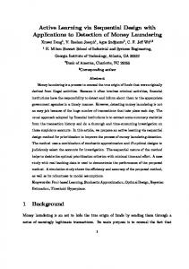
Figure 5.1: The standardized data. (Black line: the initial estimated threshold hyperplane by w0 , µ0 and σ0 .) We need to specify the prior for µ, σ, and w in (4.9) before active learning can be started. Here we use a heuristic procedure for doing this. First consider the prior for w. Assuming equal importance of x1 and x2 on the response, we would like the mean of w to be 0.5. Thus, set α0 /(α0 + β0 ) = w0 = 0.5, which implies α0 = β0 . To get a flat prior, we take 1
1
α0 = β0 = 3/2. Thus, w ∝ w 2 (1 − w) 2 . Now consider the priors for µ and σ. Choose two extreme points (i.e., two accounts) xl and xu based on the lowest and highest values of z (denoted by zl and zu ) through the mapping z = w0 x1 + (1 − w0 )x2 . We assume αl = 5% 13
suspicious level for xl and αu = 95% suspicious level for xu . Plugging them into the model (4.1), we obtain αl , 1 − αl αu zu = µ + σ log . 1 − αu zl = µ + σ log
Now, µ0 and σ0 are obtained by solving the above equations as µ0 =
αl αu zl log 1−α − zu log 1−α u l
log
αl 1−αl
αu 1−αu
− log zu − zl σ0 = αl . αu log 1−αu − log 1−α l
=
zl + zu , 2
(5.1) (5.2)
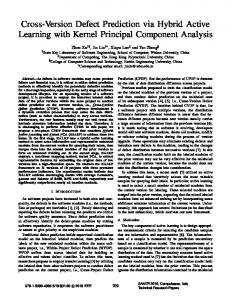
We take σµ2 as the sample variance of zi , i = 1, . . . , n, where zi = w0 xi1 + (1 − w0 )xi2 . This completes the prior specification for the three parameters. Now the active learning method can be started. Suppose our objective is to find the threshold hyperplane with α = 0.75. The initial estimated hyperplane based on only the prior is shown in Figure 5.1. The points are then selected one at a time using the procedure described in the previous section. In this example, we took k0 = 15 in (4.5). The performance of the proposed method for the first 20 points is shown in Figures 5.2 and 5.3. Figure 5.2 shows a series of estimated threshold hyperplanes using the proposed approach. The red data point in the figure means it is selected and the response is 1. The blue one means it is selected and the response is 0. At the beginning, there were significant changes in the threshold hyperplane. In about 10-15 points it started to converge showed in the bottomleft panel of Figure 5.2. The final estimated threshold hyperplane (i.e., after 20 points) is shown in Figure 5.3. The points above this hyperplane should be given higher priority and be investigated thoroughly for their suspiciousness. There are only a few remaining accounts that need a thorough investigation, which clearly shows the efficiency of the proposed method. For a new personal account in this cluster, the corresponding profile features xnew can be calculated from its transaction history. If xnew falls above the estimated threshold hyperplane, we give thorough investigation of this account; otherwise, no detail investigation is performed. 14
5 1 4 32 5
1 4 32 5
1
l4 l1 l2l3
0
6
0
1
2
x2
3
4
5 4 3 2
x2
l10
10
0
2
4
−1
−1
l5 6
0
98 l9 l8
7 l7
l6
2
4
6
4
6
4
4
5
x1
5
x1
3
3
l11
2
12 13
x2
2 1
5
1
x2
l12 l13 l15 l14 41 2 3
6
5 6
0
0
14
1 4 32 12 13 19 14
0
9158
20 10 18 16 17 11
7
−1
−1
10 11
2
4
6
0
x1
9158
7
2 x1
Figure 5.2: Active Learning via Sequential Design. (For example, yellow line l5 stands for the estimated threshold hyperplane at iteration 5.) The four panels from top left to bottom right represent the first five to the last five (i.e., iterations 15 to 20) estimated threshold hyperplanes.
15
5 4 3 2
x2
1 4
3
2 5
1
12 13 1914 0
6
7
9158
−1
20 18 16 10 17 11
0
2
4
6
x1
Figure 5.3: Comparison with the estimate based on full information. (Black line: the initial estimated threshold hyperplane by w0 , µ0 and σ0 . Pink line: the estimated threshold hyperplane after 20 points are sequentially selected. Blue dashed line: the estimated threshold hyperplane when all data are labelled.) To assess the accuracy of the proposed method, we asked the investigators at this financial institution to investigate all the 92 accounts carefully. Based on the obtained information for all the accounts, we estimated the threshold hyperplane, which is shown in Figure 5.3 as blue dashed line. We can see that it is very close to the estimated threshold hyperplane (i.e., pink line) by the active learning method. Thus, the proposed method can identify the true hyperplane by using only about 22% (≈ 20/92) of the data, which is a big saving for the financial institution. To check the efficiency of the proposed method, we also compared the proposed method with two naive methods. The first is to randomly select the next data point for getting the
16
response. The second is a sequential space-filling procedure using maxmin distance criterion (Johnson et al., 1992). The idea is to select the next data point xn+1 which maximizes the minimum distance from the chosen data points, i.e., xn+1 = arg max min dist(x, xi ), x∈X xi ∈D
(5.3)
where D is the training set containing n chosen data points xi , i = 1, . . . , n, and dist(x, xi ) is the distance between two data points x and xi . To gauge the performance of the three methods, we measure the closeness between the estimated threshold hyperplane ln,α and the optimal threshold hyperplane lα (x) when all data are labelled. The adopted measure is dist(ln,α , lα (x)) ,
X
d2i ,
(5.4)
ti ∈T
where T = {ti } is a set of points which lie evenly on the optimal threshold hyperplane lα (x), ranging from −0.5 to 1 on the coordinate of x1 . Here di is the distance of ti to the estimated hyperplane ln,α . Based on (5.4), a distance-based performance measure is defined as M 1 X distj (ln,α , lα (x)), Dist P M = M j=1
(5.5)
where M is the number of simulations, and distj represents dist(ln,α , lα (x)) for the j-th simulation. We also measured the misclassification error of these three methods. The misclassification error is estimated by (αF P + (1 − α)F N )/N , where F P is the number of false positive (i.e., a nonsuspicious account being assigned the suspicious label 1), F N is the number of false negative (i.e., a suspicious account being assigned the nonsuspicious label 0), and N is total number of accounts. As Dist P M increases, the estimated hyperplane deviates more from the true hyperplane, resulting in an increase of the misclassification error. Thus, these two measures agree with each other if the linearity assumption in the model holds. Otherwise, the misclassification error should be used because it is a more direct and relevant measure for gauging the performance. 17
0.120 0.110 0.105 0.095
0.100
Missclassification error
15 10 0
0.090
5
Dist_PM
Proposed Space Filling Random
0.115
20
Proposed Space Filling Random
0
5
10
15
20
0
n
5
10
15
20
n
Figure 5.4: Learning curves of the proposed method compared with two naive methods. Figure 5.4 shows the learning curves for the three methods in terms of Dist P M and misclassification error. Each naive method was implemented for 100 simulations. It is clear that the proposed method is much more efficient than the two naive methods. The estimated threshold hyperplane by the proposed method also moves towards the optimal threshold hyperplane more quickly and consistently. It converges in about 15 steps, and its misclassification error reaches 0.086, which is the error rate of the hyperplane estimated with the full data. The misclassification error of the proposed method is also much smaller than those of the two naive methods in each iteration. To check the linearity assumption in (4.1), we use the dispersion as a measurement of goodness-of-fit. The dispersion parameter is estimated by φˆ = X 2 /(n − p), where n is the number of observations, p the number of parameters in the model, X 2 the Pearson’s statistic P pi (1 − pˆi )), and pˆi is the estimated probability of yi = 1 defined as X 2 = ni=1 (yi − pˆi )2 /(ˆ from the proposed method. If the logit model is appropriate, then φ should be 1. Figure ˆ are around 1 in the active learning procedure. They are also much 5.5(a) shows that φ’s smaller than the 95% critical values (1.94 for n = 11, and 1.62 for n = 20) in the frequentist approach. It shows that the linearity assumption is adequate in the current study. To assess the prediction error due to model lack-of-fit, we computed the leave-one-out 18
0.18 0.16 0.14 0.10
0.12
Dispersion
1.0
1.1
1.2
Leave−one−out missclassfication error
1.3
0.20
Linear Nonlinear
12
14
16
18
20
12
n
14
16
18
20
n
(a) estimate of dispersion parameter
(b) leave-one-out misclassification error
Figure 5.5: Diagnostics for the proposed method. misclassification error, given in Figure 5.5(b) under “Linear”. The prediction errors are reasonably low. To further improve the prediction accuracy, we may use a nonlinear hypersurface such as z = wxα1 1 + (1 − w)xα2 2 with α1 , α2 ≥ 0, where α1 and α2 are estimated from the data. The leave-one-out misclassification error using this nonlinear model is plotted in Figure 5.5(b) under “Nonlinear”. It shows that use of the nonlinear model does not further reduce the misclassification error. In fact, there is a slight increase for 14 ≤ n ≤ 20. Therefore, use of the linear model is adequate in this particular problem. Both models estimated from the full data are shown in Figure 5.6, which clearly shows that the linear hyperplane is a good approximation to the nonlinear hypersurface.
6 6.1
Simulations Numerical Examples
As stated before, the proposed method is expected to be flexible and robust to model assumptions. Some simulations were conducted to study its performance. The simulated data
19
3 0
1
2
x2
4
5
6
Linear hyperplane Nonlinear hypersurface
0
2
4
6
8
x1
Figure 5.6: Comparison of the linear hyperplane and the nonlinear hypersurface estimated from the full data. were based on different models of F (x). Four models were used in the study: Logistic distribution: F (x) =
exp( z−µ ) σ z−µ , 1 + exp( σ ) z−µ σ
− (−2) , 2 − (−2) z−µ Normal distribution: F (x) = Φ( ), σ z−µ 1 1 ), Cauchy distribution: F (x) = + tan−1 ( 2 π σ
Uniform distribution: F (x) =
where z = wx1 + (1 − w)x2 and Φ is the standard normal distribution function. The true values of parameters were set as µ = 0.5, σ = 1 and w = 0.7. The response outcome at each point was generated according to F (x). An illustration of the simulated data from four models is shown in Figure 6.1. The range of x1 is kept in (-3, 3) for all the plots in Figure 20
6.1. Uniform
x2 −2
−5
0
0
2
x2
4
5
6
8
10
Logit
−1
0
1
2
−2
−1
0
x1
x1
Normal
Cauchy
1
2
x2 −20
−4
−2
−10
0
0
x2
2
10
4
6
20
−2
−3
−2
−1
0
1
2
−3
x1
−2
−1
0
1
2
x1
Figure 6.1: Illustrations of simulated data. In this simulation we chose α = 0.5 and α = 0.8 for illustration. The same performance measure in (5.5) is used here. Let k0 = 15 in (4.5). The specification of hyper-parameters is done by using the heuristic procedure discussed in the previous section. 100 simulations were performed and n = 30 points were sequentially selected in each simulation. To calculate the Dist PM in (5.5), T = {ti } in (5.4) is a set of points lying evenly on the true threshold hyperplane of each model respectively. To make T = {ti } more concentrated in the data region of the true threshold hyperplane, we adjust the spread of ti according to the value of α. When α = 0.5, ti are evenly-spaced on the true threshold hyperplane ranging from -1.5 to 1.5 on the coordinate of x1 as shown in Figure 6.1. For α = 0.8, ti are evenly-spaced on the true threshold hyperplane ranging from -0.5 to 2.5 on the coordinate of x1 . Since the random method (i.e., select the next data point randomly) in Section 5 is very naive and performed poorly, we compare the proposed method with the sequential space-filling procedure used in Section 5. Note that the accuracy of the estimated threshold 21
hyperplane is crucial in our problem for risk prioritization. We use the Dist P M to check the performance of each simulation. Performance of these two methods for two α values are shown in Figures 6.2 and 6.3.
Dist_PM 5
10
15
20
25
30
0
5
10
15
20
n
n
Normal
Cauchy
25
30
25
30
3
0.2
1
2
Dist_PM
0.6 0.4
Dist_PM
0.8
4
0
0.4 0.6 0.8 1.0 1.2 1.4
Uniform
0.6 0.8 1.0 1.2 1.4 1.6
Dist_PM
Logit
0
5
10
15
20
25
30
0
5
n
10
15
20
n
Figure 6.2: Dist P M for four models with α = 0.5. (Solid blue line: the proposed method. Dashed red line: the sequential space-filling procedure.) Clearly the proposed active learning method performs much better than the sequential space-filling procedure. Comparing Figures 6.2 and 6.3, we can see that the performance of the methods is better when α = .5. This is a well known fact in the literature that the estimation of extreme quantiles is much more difficult than with α = .5 (see, e.g., Joseph 2004). It is also clear from the figures that the proposed method is quite robust to model assumptions. In the proposed active learning approach in (4.5), one selects k0 candidate points which are closest to the estimated hyperplane. Here k0 is considered as a tuning parameter but 22
Uniform
1.5
Dist_PM
0.5
1
5
10
15
20
25
30
0
5
10
15
20
n
n
Normal
Cauchy
25
30
25
30
5 4 1
2
0.4
3
0.6
0.8
Dist_PM
6
1.0
7
1.2
0
Dist_PM
1.0
3 2
Dist_PM
4
2.0
5
2.5
Logit
0
5
10
15
20
25
30
0
5
n
10
15
20
n
Figure 6.3: Dist P M for four models with α = 0.8. (Solid blue line: the proposed method. Dashed red line: the sequential space-filling procedure.) its optimal value has not yet been addressed. An additional experiment was conducted regarding the choice of k0 . Setting α = 0.6, the proposed active learning is performed for different k0 , i.e., k0 = 1, 5, 10, 15 and k0 = N , where N is the total number of data points in the data set. k0 = 1 means active learning using stochastic approximation, whereas k0 = N means active learning using a fully D-optimal-based sequential design. 100 simulations were generated for each k0 and each model. The hyper-parameters were chosen as in Section 4. Figure 6.4 shows the simulation results . As can be seen in Figure 6.4, except for the logistic distribution the Dist P M decreases up to some value of k0 and then increases. This agrees with our initial intuition that choosing a large value of k0 may not be good if the assumed model is not correct. Our procedure assumes the logistic model. Thus, when the model is changed to uniform, normal, or Cauchy,
23
Uniform
1.0
Dist_PM
0.6
1.0
0.8
1.5
Dist_PM
2.0
1.2
Logit
20
40
60
80
0
20
40
60
k0
k0
Normal
Cauchy
80
1.0
1.5
Dist_PM
0.7 0.5 0.3
Dist_PM
2.0
0.9
0
0
20
40
60
80
0
k0
20
40
60
80
k0
Figure 6.4: Performance with different k0 . (Solid green line: n = 10; Dashed blue line: n = 20.) the method did not do well with a large k0 . As expected, the performance did not deteriorate with k0 when the true model is logistic. It is also clear that k0 = 1 is a bad choice as the Dist P M is the largest in all cases. Thus, using a purely stochastic approximation method for active learning is not good in this particular problem. It is not clear what is the best value of k0 . The simulation results suggest choosing k0 to be 20%-50% of N .
6.2
Comparison with Support Vector Machine
Active learning using support vector machine (SVM) for classification has been proposed with several versions (Schohn & Cohn, 2001; Campbell et al., 2001; Tong & Koller, 2001). The basic idea is to label points that lie closest to the SVM’s dividing hyperplane. It is known that the hyperplane in SVM converges to the Bayes rule P (Y = 1|x) = α, where 24
α = 0.5. The proposed active learning via sequential design can also converge to the threshold hyperplane when α = 0.5. To start the active learning with SVM, some initial sample of data points are needed. Therefore, to have a fair comparison, we used eight points as the initial sample chosen based on the stratified random sampling. It is implemented as follows. With the initial guess on the parameters µ0 , σ0 and w0 , we can get z = w0 x1 + (1 − w0 )x2 . Then we divide the range of z into four strata as (−∞, µ0 −1.6σ0 ), [µ0 −1.6σ0 , µ0 ), [µ0 , µ0 +1.6σ0 ) and [µ0 + 1.6σ0 , +∞). Since each point x can be mapped into the z value, we randomly choose two x0 s in each stratum according to the corresponding z value. The choice of the constant ±1.6 is based on the asymptotic optimality of the estimators under logistic distribution (see, e.g., Neyer 1994). The hyper-parameters were chosen as before. 100 simulations were generated for comparison. Uniform
3
Dist_PM
1
1
15
20
25
30
35
10
15
20
25
n
n
Normal
Cauchy
30
35
30
35
3 2
0
1
1
2
3
Dist_PM
4
4
5
5
10
Dist_PM
2
3 2
Dist_PM
4
4
5
5
Logit
10
15
20
25
30
35
10
n
15
20
25 n
Figure 6.5: Comparison of Active Learning with SVM. Solid blue line: the proposed active learning. Dashed red line: active learning with SVM.
25
The Dist P M values are plotted in Figure 6.5. We can see that the Dist P M values of the proposed active learning are much smaller than that of the active learning with SVM. Moreover, the proposed active learning is quite stable, whereas the SVM is quite unstable for small n. The SVM is not robust because adding one more point into the training set can cause big changes in the SVM’s dividing hyperplane. Thanks to the use of the Bayesian approach, the estimation in the proposed active learning is stable. The proposed active learning seems to converge within 20 steps, while the active learning with SVM needs at least 10 more steps to achieve similar performance. The improvement is even more pronounced with heavy tail distributions like Cauchy. Thus in this particular problem, the proposed active learning outperformed active learning with SVM in all aspects including accuracy, stability, and robustness.
7
Discussions and Conclusions
In this article, we propose an active learning via sequential design and report its application to a real world problem in money laundering detection. Due to the large amount of transactions and various business categories, it is crucial to find an efficient way to get the threshold hyperplane for prioritization. The proposed method is efficient and accurate for estimating the threshold hyperplane, and its performance is robust to model assumptions. It can help investigation to put more effort on those accounts with great importance. Therefore, this approach can significantly improve the productivity of money laundering detection. The proposed active learning method uses a combination of stochastic approximation and optimal design methods. From the sequential design perspective, we have shown that the proposed method works better than either of stochastic approximation and optimal design. Through simulations we have also shown that the proposed method outperforms active learning methods using SVM. Regarding the choice of k0 (i.e., the number of candidate points in (4.5)), the simulation study suggests choosing k0 to be 20%-50% of N . The proposed method is described for two profile features x = (x1 , x2 )T and the threshold hyperplane is linear in x. When the linearity assumption is reasonable, it can be easily 26
extended to higher dimensions. In multivariate situations with x = (x1 , x2 , . . . , xp )T , we can define a synthetic variable z as a convex combination of the profile features, i.e., z = Pp Pp i=1 wi xi , where wi ≥ 0 and i=1 wi = 1. Then, the active learning criterion (4.5) can be applied to select the next data point. Regarding the choice of the priors, we use the normal prior for the location parameter µ, the exponential prior for the scale parameter σ, and the Dirichlet prior for the weight parameters w = (w1 , w2 , . . . , wp )T . For this to work, we need to assume monotonic effects for each of the profile features. This assumption seems reasonable in problems we have encountered so far. If the threshold hyperplane has a nonlinear form in the profile features x, the linearity assumption in the model may lead to lack-of-fit and poor prediction accuracy. This can be alleviated by using a nonlinear model as in Section Pp αi 5, i.e., by taking z = i=1 wi xi , where αi ≥ 0 for all i = 1, . . . , p. Another strategy of incorporating the nonlinearity is to consider the so-called “kernel trick” (Sch¨olkopf and Smola, 2002) on the synthetic variable z for the logit model in (4.1), i.e. z can be expressed as an inner product in the reproduced kernel Hilbert space (Wahba, 1990). Generalizing the active learning criterion (4.5) for the nonlinear threshold surface is an interesting topic for future research. The proposed active learning via sequential design is flexible in estimating threshold hyperplane for different α. On the other hand, the standard support vector machine is mainly for classification problem with α = 0.5. Lin et al. (2002) proposed a modified support vector machine to account for α different from 0.5. However, the active learning using the modified support vector machine is not available in the literature. Although the proposed method was motivated by the problem of detecting money laundering, the sequential nature of the proposed method can be linked with other applications such as sensitivity experiments (Neyer, 1994), bioassay experiments (McLeish and Tosh, 1990), contour estimation in computer experiments (Ranjan et al., 2007), and identification of lead compounds in drug discovery (Abt et al., 2001). Abt et al. (2001) used a twostage sequential approach to minimize the number of physical tests and select a set of good candidate compounds. Their work shares two common features with ours: large number of independent variables, and high cost of measuring the potencies of chemical compounds. 27
These features are common place in other fields. For example, in signal processing or image recognition, often times the observations are available but not labelled or investigated to get the response. Each observation can be a functional curve or consists of many data points in a high dimensional space. Due to the complexity of the observations, getting the responses is time-consuming and costly. By transforming the data into several uncorrelated monotonic profile features, the proposed active learning method can be used to exploit the level of interest of the response efficiently.
Acknowledgements We are greatly thankful to the Associate Editor and the referees, whose constructive comments helped us to improve the contents and presentation of the paper. The research of Deng, Joseph and Wu was supported in part by a grant from the U. S. Army Research Laboratory and the U. S. Army Research Office under contract number W911NF-05-1-0264.
Appendix Equivalence between (4.7) and (4.8). ˆ n , x1 , x2 , . . . , xn , x) = I(θ ˆ n , x1 , x2 , . . . , xn ) + κx η x η T , where κx = eg(x) /(1 + From (4.6), I(θ x ∂g(x) g(x) 2 . Under mild regularity conditions, the Fisher information matrix e ) and η = x
∂θ
ˆ n , x1 , x2 , . . . , xn ) is positive semi-definite and nonsingular. Therefore, applying the idenI(θ tity det(A + cxxT ) = det(A)(1 + cxT A−1 x), we obtain ˆ n , x1 , x2 , . . . , xn , x)) = det(I(θ ˆ n , x 1 , x 2 , . . . , x n ) + κx η η T ) det(I(θ x x ˆ n , x1 , x2 , . . . , xn )η ). ˆ n , x1 , x2 , . . . , xn ))(1 + κx η T I −1 (θ = det(I(θ x x ˆ n , x1 , x2 , . . . , xn )η x . ˆ n , x1 , x2 , . . . , xn , x)) is the same as minx κx η T I −1 (θ Thus minx det(I(θ x Now under the constraint in (4.7), κx = α(1 − α) is a constant. Thus we get (4.8). Note that η x = (−1/σ, − log(α/(1 − α))/σ, (x1 − x2 )/σ)T under constraint in (4.7). ¤
28
References Abt, M., Lim, Y., Sacks, J., Xie, M. and Young. S. (2001), “A Sequential Approach for Identifying Lead Compounds in Large Chemical Databases”, Statistical Science, 16, 154–168. Albert, A. and Anderson, J. A. (1984), “On the Existence of Maximum Likelihood Estimates in Logistic Regression Models,” Biometrika, 71, 1–10. Campbell, C., Cristianini, N. and Smola, A. (2000), “Query Learning with Large Margin Classifiers,” In Proceedings of 17th International Conference on Machine Learning, pages 111–118. Cohn, D. A., Ghahramani, Z. and Jordan, M. I. (1996), “Active Learning with Statistical Models,” Journal of Artificial Intelligence Research, 4, 129–145. Fedorov, V. V. (1972), Theory of Optimal Experiments, Academic Press, New York. Fukumizu, K. (2000), “Statistical Active Learning in Multilayer Perceptrons,” IEEE Transactions on Neural Networks, 11(1), 17–26. Johnson, M., Moore, L. and Ylvisaker, D. (1990), “Minimax and Maximin Distance Design,” Journal of Statistical Planning and Inference, 26, 131–148. Joseph, V. R. (2004), “Efficient Robbins-Monro Procedure for Binary Data,” Biometrika, 91, 461–470. Joseph, V. R., Tian, Y. and Wu, C. F. J. (2007), “Adaptive Designs for Stochastic RootFinding,” Statistica Sinica, 17, 1549–1565. Kiefer, J. (1959), “Optimum Experimental Designs,” Journal of the Royal Statistical Society, Series B , 21, 272–304.
29
Lewis, D. and Gale, W. (1994), “A Sequential Algorithm for Training Text Classifiers,” In Proceedings of the Seventeenth Annual International ACM-SIGIR Conference on Research and Development in Information Retrieval , pages 3–12, Springer-Verlag. Lin, Y., Lee, Y. and Wahba, G. (2002), “Support Vector Machines for Classification in Nonstandard Situations,” Machine Learning, 46, 191–202. MacKay, D. J. C. (1992), “Information-Based Objective Functions for Active Data Selection,” Neural Computation, 4(4), 590–604. McLeish, D. L. and Tosh, D. (1990), “Sequential Designs in Bioassay,” Biometrics, 46, 103–116. Neyer, B. T. (1994), “D-Optimality-Based Sensitivity Test,” Technometrics, 36, 61–70. Pukelsheim, F. (1993), Optimal Design of Experiments, New York: John Wiley & Sons. Ranjan, P., Bingham, D. and Michailidis, G. (2007), “Sequential Experiment Design for Contour Estimation from Complex Computer Codes”, Technometrics, accepted. Santner, T. J. and Duffy, D. E. (1986), “A Note on A. Albert and J. A. Andersons Conditions for the Existence of Maximum Likelihood Estimates in Logistic Regression Models,” Biometrika, 73, 755–758. Schohn, G. and Cohn, D. (2000), “Less is More: Active Learning with Support Vector Machines,” In Proceedings of the Seventeenth International Conference on Machine Learning. Sch¨olkopf, B. and Smola, A. (2002). Learning with Kernels. MIT Press, Cambridge. Silvapulle, M. J. (1981), “On the Existence of Maximum Likelihood Estimators of the Binomial Response Model,” Journal of the Royal Statistical Society, Series B , 43, 310–313. Silvey, S. D. (1980), Optimal Design. London: Chapman and Hall. 30
Tong, S. and Koller, D. (2001), “Support Vector Machine Active Learning with Applications to Text Classification,” Journal of Machine Learning Research, 2, 45–66. Vapnik, V. N. (1998), Statistical Learning Theory, New York: John Wiley & Sons. Wahba, G. (1990), Spline Models for Observational Data. SIAM, Philadephia. Wu, C. F. J. (1985), “Efficient Sequential Designs with Binary Data,” Journal of the American Statistical Association, 80, 974–984. Ying, Z. and Wu, C. F. J. (1997), “An Asymptotic Theory of Sequential Designs Based on Maximum Likelihood Recursions,” Statistica Sinica, 7, 75–91. Young, L. J. and Easterling, R. G. (1994), “Estimation of Extreme Quantiles Based on Sensitivity Tests: A Comparative Study,” Technometrics, 36, 48–60.
31