Active Semi-Supervised Approach for Checking App Behavior Against Its Description Siqi Ma1 , Shaowei Wang1 , David Lo1 , Robert Huijie Deng1 , and Cong Sun2 1
School of Information System, Singapore Management University School of Computer Science and Technology, Xidian University Email:{siqi.ma.2013,shaoweiwang.2010,davidlo,robertdeng}@smu.edu.sg
[email protected] 2
Abstract—Mobile applications are popular in recent years. They are often allowed to access and modify users’ sensitive data. However, many mobile applications are malwares that inappropriately use these sensitive data. To detect these malwares, Gorla et al. propose CHABADA which compares app behaviors against its descriptions. Data about known malwares are not used in their work, which limits its effectiveness. In this work, we extend the work by Gorla et al. by proposing an active and semi-supervised approach for detecting malwares. Different from CHABADA, our approach will make use of both known benign and malicious apps to predict other malicious apps. Also, our approach will select a good set of apps for experts to label as malicious or benign to form a set of labeled training data – it is an active approach. Furthermore, it will make use of both labeled data (known malicious or benign apps) and unlabeled data (unknown apps) – it is a semi-supervised approach. We have evaluated our approach by using a set of 22,555 Android apps. Our approach achieves a good performance in detecting malicious apps with a precision of 99.82%, recall of 92.50%, and F-measure of 96.02%. Our approach improves CHABADA by 365.8%, 64.8%, 209.6% in terms of precision, recall, and Fmeasure. Keywords—App Mining, Malware Detection, Deviant Behavior Detection, Text Mining, Classification
I.
I NTRODUCTION
With the rapid growth of smartphones, mobile applications (apps for short) of different categories, such as social, financial, game, lifestyle, etc., are available for download from different application markets, such as Android’s Google Play Store and other third-party markets. Android applications often provide the detailed information, including application names, application descriptions, categories that they belong to, ratings from users, etc. Among these information, users identify apps that they want according to the application description, which means that the application should behave according to what the description of the application specifies. Gorla et al. [3] propose an approach to detect outliers, named CHABADA, which compares app behaviors against its descriptions. In their work, data about known malwares are not made use of to identify other malwares, which limits the effectiveness of their approach. Malware data could be used to improve the effectiveness of malware detection. In this paper, we propose an approach that automatically detects malicious apps by matching app description and app behaviors using semi-supervised learning and active learning. We utilize both malicious and benign apps’ descriptions and API method usages to train a classifier to predict malicious
apps with Ensured Collaborative Active and Semi-Supervised Labeling (ECASSL) [10]. ECASSL combines active learning and semi-supervised learning. Our approach will select a good set of apps for experts to label as malicious or benign to form a set of labeled training data – it is an active approach. Also, it will make use of both labeled data (known malicious or benign apps) and unlabeled data (unknown apps) – it is a semisupervised approach. We have evaluated our solution on 22,555 apps of different categories, which contains 22,383 benign apps and 172 malicious apps. We evaluate our approach in two ways. Firstly, we perform an experiment by following stratified 10-fold cross validation, and compare the results of our approach with that of CHABADA [3]. The results show that our detection approach could improve CHABADA by 365.8%, 64.8%, 209.6% in terms of precision, recall and F-measure respectively. Secondly, to determine that our approach could work with limited training data, we run an experiment with different amount of training data. We vary the amount of training data from 10% to 90% of the entire data with 10% interval. Our results show that we could achieve a precision of 100%, recall of 91.23%, and F-measure of 95.41%, when using 10% of the entire data as training data. The contributions of our work are as follows: • We propose a solution that combines semi-supervised learning and active learning, which aims to use small set of labeled data to achieve a good classifier with high accuracy. We leverage features extracted from description and binary code to detect the suspicious behaviors of an app. •
We have performed an empirical evaluation of our approach. The results show that our approach could achieve a higher F-measure than the previous approach, proposed by [3]. Moreover, our approach still has a higher accuracy with only 10% of labeled data, which demonstrate that our approach could detect malicious apps effectively, even with a small set of labeled data.
The structure of this paper is as follows. We give the overall framework of our approach in Section II. In Section III, we introduce the preprocessing strategies in detail. We present the method to extract features from app descriptions and installation files in Section IV. We illustrate our classifier learning algorithm and label prediction strategy in Section V. Our evaluation results are presented in Section VI. We
III. Training Phase
Deployment Phase
Application Description
Application Installation File (.apk)
Application Description
Application Installation File (.apk)
Description Preprocessor
App Preprocessor
Description Preprocessor
App Preprocessor
Feature Extractor
Feature Extractor
Classifier Learner
Classifier Model
Label Predictor Category Label
Fig. 1.
Our proposed framework
discuss related work in Section VII. Section VIII closes with conclusion and future work. II.
OVERALL F RAMEWORK
We present the overall framework of our approach in Figure 1. Our framework contains two phases: training phase and deployment phase. For the training phase, the framework takes as inputs basic application information, which are apps descriptions and apps installation files (i.e., “.apk” files) and outputs a classifier model that is able to differentiate malicious apps and benign apps. This learned classifier model will then be passed to the deployment phase. In the deployment phase, given an unknown application (i.e., it is unclear if it is a benign or malicious app) with its basic information (i.e., application description and application installation file), we preprocess the basic information and apply the classifier model generated from the training phase to detect whether this application is a malicious app or a benign app automatically. A. Training Phase In the training phase, we have four components: Description Preprocessor, App Preprocessor, Feature Extractor, and Model Learner. Description Preprocessor and App Preprocessor perform preprocessing on the description and installation file of each given app. Then, we extract the features of every app by using the Feature Extraction component (see Section IV for details). Finally, we train a classifier by taking the feature vectors of apps and the app labels (i.e., malicious or benign) as inputs. Here, we choose a machine learning algorithm to generate the classifier for detecting malicious apps (see Section V-A for details). The classifier would be used in the deployment phase. B. Deployment Phase In the deployment phase, we also have 4 components: Description Preprocessor, App Preprocessor, Feature Extractor, and Label Prediction. We apply the same preprocessor and feature extraction steps on the unknown app. Then, the classifier model that is generated in the training phase is used to process the feature vector of the app and predict whether this app is malicious or benign (see Section V-B for details). This last step is performed by the Label Prediction component.
D ESCRIPTION & A PP P REPROCESSOR
A. Description Preprocessor We use standard techniques in information retrieval (IR) and natural language processing (NLP) to preprocess the application description. There are two steps: stop-word removal, and stemming. Stop-Word Removal: Stop words are words that appear very often in textual documents (e.g., “am”, “on”, “it”, etc.). Since these words appear too often, they are of little help in differentiating one document from another. They are normally removed from documents before they are processed by a text analysis tool. We use the stop-word list provided by RANKS.NL1 and remove stop words specified in the list from app descriptions. We also remove numbers, URLs, email addresses, and punctuation marks. Stemming: We apply Porter Stemmer2 to do stemming on all non-stop words that appear in the app descriptions. Stemming is to convert a word to its root form. For example, words “stemmer”, “stemming”, “stemmed” are all stemmed to the root “stem”. Note that a root word is not necessarily a valid English word. B. App Preprocessor We use the App Preprocessor component to preprocess the application installation files (i.e., “.apk” files). In our paper, app behaviors are described by its API method usage, which can be obtained by decompiling the “.apk” files. We use apktool3 to decompile every “.apk” file and get smali files for every app. Each smali file defines the API methods that are used by the application. IV.
F EATURE E XTRACTOR
In order to learn a classifier, we extract two kinds of features for every application: topic features from the application description, and API features from the application bytecode (i.e, .apk file). The workflow of our feature extraction component is shown in Figure 2. The feature extractor component contains three sub-components: Description Feature Extractor, App Feature Extractor, and Feature Vector Generator. A. Description Feature Extractor An application description, typically contains one or more topics or key concepts. For example an app can be related to speed game, or music, etc. To extract topics (i.e., abstractions of words in the descriptions), our Description Feature Extractor inputs the preprocessed app description to a topic modeling technique which will automatically infer a set of topics that appear in the app description. We use a well-known topic modeling algorithm namely Latent Dirichlet Allocation (LDA) [2]. In LDA, a topic contains a lot of words that appear in the documents, and each word could be regarded as an attribute of this topic. Every document is relevant to a number of topics 1 http://www.ranks.nl/stopwords 2 http://tartarus.org/martin/PorterStemmer/java.txt 3 http://code.google.com/p/android-apktool/
Application Descriptions
Feature Extractor Description Feature Extractor
Text
LDA-GA
Topics Feature Vector Generator
Application Installation Files
Feature Vectors
App Feature Extractor .smali
Fig. 2.
Method Filter
Sensitive API Usage
According to the probabilities, Topic 61 is the most related topic, which contains words such as “screen”, “widget”, “home”, “add”, etc. From the words, we can infer that the topic is related to the concept “screen widget”. TABLE II.
E XAMPLES OF TOPICS AND THEIR REPRESENTATIVE WORDS WE OBTAINED FROM APP DESCRIPTIONS
Package Name
Category
Coin Pirates
Cards
Fancy Widgets Unlocker
Personalization
Architecture and workflow of our feature extractor component
with a corresponding probability. Table I shows some topic samples with their attribute words which are extracted from the descriptions of Android applications. For topic 1, a set of words, such as “car”, “speed” and “race” is grouped together. Although LDA does not give a name to this topic, we can infer that this topic is related to speed game. An application will be assigned to topic 1 if the relevant attribute words of topic 1 occur many times in its description. LDA accepts a number of parameters, e.g., the number of topics (κ), α, β, the number of iterations, etc. It is not easy to correctly determine optimal values of these parameters. In [3], they freely set the number of topics as 30, however, it is not clear if 30 is the best value for this parameter. An optimal LDA configuration is essential to train a good classifier. In this work, we make use of LDA-GA [14] to obtain a nearoptimal LDA configuration. The LDA-GA (Latent Dirichlet Allocation-Genetic Algorithm) algorithm combines LDA algorithm with genetic algorithm (GA) [5] to imitate the process of “survival of the fittest” to generate near optimal solutions. LDA-GA makes use of the concept of silhoutte coefficient to assess the fitness of a set of parameters. The value of silhouette coefficient is always between -1 and 1. When the value of the silhouette coefficient of a word is close to 1, the word is assigned to the appropriate topic. Conversely, if the value of the silhouette coefficient is close to -1, the word is in a wrong topic. TABLE I. Topic Id 1 2 3 4 5
S OME SAMPLE TOPICS WITH THEIR ATTRIBUTE WORDS Short Description Speed Game Music Media Shopping Web Social
Attribute Words car, speed, race, fast, super, control, ... file, download, audio, music, media, ... shop, place, famili, order, visit, pick, ... keyword, histori, websit, brows, ad, ... call, messag, contact, email, voic, text, ...
After running the LDA-GA algorithm, we obtain a set of near-optimal values for the LDA configuration. Note that a LDA computes the probability of a document to belong to a topic. Following [3], we define that an app description belongs to a topic if its probability for that topic is at least 5%. Since an app can be related to many topics, we do not specify a maximum number of topics that can be assigned to an app description. Table II shows an example of topics we obtained from descriptions of different apps. As an example, Fancy Widgets Unlocker, shown in Table II. It belongs to the following topics : • Topic 61 with the probability of 11.4%. •
Topic 62 with the probability of 9.74%.
•
Topic 27 with the probability of 7.22%.
Topic Topic Topic Topic Topic Topic Topic
Id (Topic Attributes) 15 (want, like, need, try, ...) 30 (level, game, challeng, score, ...) 50 (game, fun, plai, challeng, ...) 27 (try, free, power, featur, ...) 61 (screen, widget, home, add, ...) 62 (instal, devic, displai, android, ...)
B. App Features Extraction After the preprocessing phase, each .apk file is converted into a set of API methods that it invokes. Since not all API methods are important ones, we only focus on a number of sensitive API methods, and filter the API methods by using app feature extractor. The sensitive API methods that we use in this study are based on those that are identified in [3]. They decide an API method to be sensitive or not based on the Android permission setting that is required to run the API method. They collect 304 sensitive API methods. In this work, we regard sensitive API methods with the same name but different parameters as the same API method. We do this step since API methods of the same name but different parameters are typically very similar to one another. Considering their potential high similarities, rather than treating them as separate methods, it is better to treat them as the same method. For example, method android.accounts.AccountManager.getAuthToken is used to get an authentication token of a specific type for a particular account, and it has three variants that take different parameters. These three methods perform the same activity, and thus we use android.accounts.AccountManager.getAuthToken to represent all of the three methods. After grouping sensitive methods of the same name, we have a total of 270 sensitive API methods. C. Feature Vector Generator Give a app’s topic features (i.e., topics in the description of the app) and API features (i.e., sensitive API methods used by of the app), the Feature Vector Generator sub-component produces a vector that combines these two types of features. Each element in the vector is a pair that contains a topic (that appears in the app’s topic features) and an API method (that appears in the app’s API features). We extract these features since some topic-API combinations are common and characterize benign apps, while other topic-API combinations are rare to indicate suspicious or even malicious applications. Example: Suppose an app’s API features are AP I1 and AP I4 , and its topic features are T opic1 and T opic3 . We obtain these API and topic features, Feature Vector Generator will generate the following feature vector: h(T opic1 , AP I1 ), (T opic1 , AP I4 ), (T opic3 , AP I1 ), (T opic3 , AP I4 )i.
V.
C LASSIFIER L EARNER & L ABEL P REDICTION
This section describes the Classifier Learner and Label Predictor components. Classifier Learner is run in the training phase, and Label Predictor is run in the deployment phase. A. Classifier Learner Classifier learner is used for training a classifier model to differentiate malicious apps from benign apps. It takes as inputs a set of feature vectors and labels (i.e., benign or malicious) of apps in a training dataset. Each feature vector contains pairs of API method used by an app and topic of the app’s description. Thus, the classifier learner could learn to differentiate topic-API pairs that correspond to benign applications and those that correspond to malicious applications. Dataset PseudoLabeled Data
SVM Algorithm
Margin Sampling
Update Dataset
Labeled Data Pseudo Label Generation
SVM Algorithm
Unlabeled Data
Fig. 3.
Classifier learning process
In our paper, we use support vector machines (SVM), which has been shown to perform very well for text classification [17]. Furthermore, instead of using supervised learning that requires all training data to be labeled, we choose to use the Ensured Collaborative Active and Semi-Supervised Labeling (ECASSL) algorithm, which combines semi-supervised learning (SSL) and active learning (AL) and is built on top of SVM [10]. The classifier learning process that we follow in this work is illustrated in Figure 3. The steps in the process is described as follows: 1. Build an initial set of pseudo labeled apps. We make use of the tri-training algorithm [19] to generate an initial set of pseudo labeled apps to enrich the input labeled apps which are small in number. In tri-training algorithm, three classifiers (i.e., decision trees4 ) are built, and a pseudo label is assigned to an app only if any two of the classifiers agree on the label of the app.
4. Manually label the selected apps. Apps selected in step 3 will be manually labeled. After they are labeled, the sets of unlabeled and labeled apps are updated. 5. Run SVM algorithm to build a refined model. Taking the updated set of labeled apps, we use SVM to learn a second classifier SVM 2. 6. Generate additional pseudo labels. For every unlabeled app, we generate new pseudo labels Label 1 and Label 2 using SVM 1 and SVM 2, respectively. Then, we take all apps which have the same Label 1 and Label 2 as new pseudolabeled apps. We repeat the above-mentioned steps t times by using the new set of pseudo labeled apps. The process will stop when the labeling budget Nbudget has been reached, and output SVM 1. The intuition behind the classifier is that benign apps are likely to have only commonly used topic-method pairings, while malicious apps are likely to have one or more rare topic-method pairings. To illustrate this intuition, consider the following examples. Consider two applications CP5 and FWU6 . CP is a game and make use of sensitive API methods related to network connection. Apps with the same topic (i.e., game apps) normally use network connection. Thus, it can be inferred that CP is a benign app. On the other hand, FWU is an app that provides a clock and weather widget, and it calls API methods that obtain device and subscriber ids, and listens to, the telephony service on the device. It is not normal for a clock and weather app to perform these actions. From these uncommon behaviors, captured by uncommon topic-API pairings, it can be inferred that FWU is a malicious app. B. Label Prediction Given a new unlabeled app, the Label Predictor outputs a label (i.e., malicious or benign) based on the classifier model generated by Classifier Learner. The unlabeled app is first processed by the Feature Extractor component which generates a feature vector for this app. Then, the Label Predictor inputs this feature vector into the classifier model and assigns a label with the highest likelihood to the app. VI.
E VALUATION
In this section, we present the experimental setting, research questions and their results, and some threats to validity. A. Datasets & Experiment Settings
2. Run SVM algorithm to build an initial model. Taking the initial set of pseudo labeled data and labeled data, we employ SVM to build a classifier, SVM 1. 3. Perform margin sampling to select some apps to label. We perform an iteration of active learning. In an iteration, we employ the margin sampling algorithm [15] to select the N top budget unlabeled apps which are the most close to the t hyperplane of SVM 1, where Nbudget is the labeling budget (i.e., maximum number of apps to label) and t is the number of iterations. 4 We
choose decision tree algorithm, since the performance of the decision tree is better than other classifiers.
We use the dataset provided by Gorla et al. [3], which includes the application description, and the application API method usage. In their dataset, there is 22,555 apps with 172 malicious apps and 22,383 benign apps. Our approach is mainly implemented in Java. We use JGibbLDA [18] and JGAP [1] to implement the LDA-GA algorithm and obtain a set of semi optimal configuration7 to run LDA. By default, we set the value of t, which controls the number of active learning iterations, to 15. 5 The
name of the app has been anonymized. name of the app has been anonymized. 7 α = 0.6, β = 0.3, and the number of topic κ = 95 6 The
B. Metrics To measure the effectiveness of a malware detection technique, we use four standard metrics: precision, recall and Fmeasure. They are defined based on the true positive (TP8 ), true negative (TN9 ), false positive (FP10 ), and false negative (FN11 ). In a classification task [13], precision for a class is defined as the number of true positives divided by the total number of data points (in our case: apps) labeled as positive. Recall is defined as the number of true positives divided by the total number of data points (in our case: apps) that are actually positive (in our case: malicious). F-measure represents the harmonic mean of precision and recall. Higher values of precision, recall, and F-measure indicate higher detection quality. F-measure is typically used as a summary measure to combine precision and recall. C. Research Questions To evaluate our approach, we conduct experiments to answer the following main research questions: RQ1 How effective is our approach for malware detection? Can our approach outperforms the state-of-the-art approach? To answer this research question, we compare the effectiveness of our approach and that of CHABADA [3], in terms of precision, recall and F-measure. We evaluate our approach by performing a stratified 10-fold cross validation on the same dataset. We split the entire set of 22,555 applications into 10 subsets. We run the experiment 10 times, each time we select a different subset for testing, and the other 9 subsets as the training data. We report the average performance over the ten experiments. RQ2 How does the performance of our approach vary for various amount of training data? In 10-fold cross validation, we use 90% of the data for training and 10% for testing. This setting assumes that a large amount (i.e., 90%) of labeled training data is available. Our approach employs active learning and semi-supervised learning. The aim of using these techniques is to reduce the amount of training data labeled by experts. In this research question, we would like to investigate whether our approach can work well with a reduced amount of training data. To answer this research questions, we run multiple experiments by varying the amount of training data from 10% to 90% of the entire data, with 10% interval. We perform our experiment 9 times with different amount of training data.
TABLE III.
C OMPARISON BETWEEN OUR APPROACH AND CHABADA Precision 99.82% 21.43%
Our approach CHABADA
Recall 92.50% 56.10%
F-measure 96.02% 31.01%
TABLE IV.
R ESULT USING DIFFERENT AMOUNT OF LABELED DATA USED FOR TRAINING . P = P RECISION , R = R ECALL , F = F- MEASURE .
10% 20% 30% 40% 50%
P 100% 90.33% 100% 99.89% 100%
R 91.23% 92.23% 92.48% 92.97% 92.81%
F 95.41% 91.76% 96.09% 96.31% 96.27%
P 99.49% 99.98% 100% 100%
60% 70% 80% 90%
R 93.62% 93.31% 92.87% 93.42%
F 96.46% 96.52% 96.30% 96.60%
value of t from 1 to 15 and evaluate the effectiveness of our approach, in terms of precision, recall, and F-measure, for each of the t value. D. Experiment Results In the following paragraphs, we describe our experiment results which answer the research questions presented in the previous sub-section. 1) RQ1: Effectiveness of our approach in detecting malicious apps: The results are shown in Table III. The results demonstrate that our approach improves CHABADA on all metrics. The precision, recall, and F-measure values of our approach are 99.82%, 92.50%, 96.02%, respectively. Compared with CHABADA, who gets the precision, recall, and Fmeasure scores of 21.43%, 56.10%, and 31.01% respectively, our approach improves CHABADA by 365.8%, 64.8%, and 209.6%, respectively. 2) RQ2: Training data sensitivity analysis: The results are shown in Table IV. We notice that even with 10% of the entire dataset as the training data, our approach could detect malware effectively, with precision of 100%, recall of 91.23%, and Fmeasure of 95.41%. 3) RQ3: Effect of the varying t: The results are shown in Figure 4. From the figure, we can note that the effectiveness of our approach is substantially poorer when we use a small number of iterations. The performance is better when the number of iterations are set to 10 or above. Increasing the number of iterations from 10 to a larger number does not improve the effectiveness of our approach by much. F -m e a su r e P r e c is io n R e c a ll 1 .0
0 .9
RQ3 How does the performance of our approach vary for different setting of t? Our approach accepts one parameter t. t is a parameter to control the number of active learning iterations. In this research question, we would like to investigate the effect of varying the value of t. To answer this research question, we vary the 8 TP:
an app that is a malicious app and is classified as a malicious app. an app that is a benign app and is classified as a benign app. 10 FP: an app that is a benign app and is classified as a malicious app. 11 FN: an app that is a malicious app and is classified as a benign app 9 TN:
0 .8
0 .7
0
5
1 0
1 5
N u m b e r o f I te r a tio n Fig. 4. Impact of varying the value of t on our approach in terms of precision, recall and F-measure
E. Threats to Validity Threats to internal validity relates to errors in our experiments and datasets. We make use of the dataset made available by Gorla et al. and thus share the same threats to internal validity as them. We have checked our code for bugs and errors, however, there could be bugs and errors that we miss. Threats to external validity relates to the generalizability of our findings. We have only investigated the effectiveness of our approach on a dataset containing 22,000+ apps. These apps might not represent all possible apps. In the future, we plan to reduce the threats to external validity further by investigating additional apps. Threats to construct validity relates to the suitability of the evaluation metrics that we use. We make use of precision, recall, and F-measure. These metrics are standard data mining metrics [4] and they have been used in various software engineering studies, e.g., [6], [9]. Thus, there would be little threat to construct validity. VII.
R ELATED WORK
Only few recent techniques leverage app description information to detect malwares. WHYPER [12] detects malware by matching app description and its required permissions. Gorla et al. extend WHYPER, by proposing CHABADA [3], which identifies outliers by matching app description and its API method usage. In this work, we extend CHABADA. Similar to CHABADA, we analyze app description and API usages. However, rather than only using information from benign apps to create a model, our approach also uses information of malicious apps. To limit the amount of training data needed, we use semi-supervised learning and active learning to build a classifier, which can achieve high accuracy even with few labeled data. Many software engineering research works make use of classification algorithms to automate various software engineering tasks [7], [16], [8], [11]. Jalbert and Weimer propose an approach that extracts features from bug reports and automatically predict if a bug report is a duplicate of a previously submitted bug report [7]. Tian et al. predict finegrained severity labels of bug reports from open source bug tracking systems [16]. Kochhar et al. propose an approach that can predict fine-grained categories of issue reports (e.g., bug, request for improvement, documentation, refactoring, etc.) [8]. Lo et al. extracts iterative patterns as features to be input to a classification algorithm to predict if an execution trace is faulty or not [11]. Similar to the above mentioned approaches, we also employ a classification algorithm. However, we address a different problem: we use the classification algorithm to predict if an app is a malware or not. We need to extract a different set of features than those extracted in the above mentioned approaches. Also, while most of the above mentioned approaches are using fully supervised classification algorithms, we are using active learning and semi-supervised learning to make our approach performs well even when there is a limited number of training data.
extracts topics from app description and used API methods of an app. It then constructs a feature vector to characterize an app where each element of the vector is a topic-API pairs. Feature vectors of apps are then used to train a classifier model. We make use of the ECASSL classification algorithm, which combines both semi-supervised learning and active learning, and is built on top of SVM. We have evaluated our approach on a set of data with 22,555 benign apps and 172 malicious apps. We compare the results of our approach with CHABADA and show that our approach could improve CHABADA by 209.6% in terms of F-measure. Furthermore, we have performed a sensitivity analysis by varying the amount of training data and show that our approach can achieve an F-measure of 95.41% even when only 10% of the entire data are selected as training data. In the future, we plan to enhance our approach with a dynamic analysis component to improve its effectiveness further. We also plan to reduce the threats to external validity by investigating an even larger number of apps. R EFERENCES [1] [2] [3] [4] [5]
[6]
[7] [8] [9] [10] [11]
[12]
[13]
[14]
[15] [16]
[17]
VIII.
C ONCLUSION AND F UTURE W ORK
This paper proposes an automated approach to detect malicious apps. To realize this, our approach processes both app description and the .apk file of an app. Our approach
[18] [19]
Jgap homepage. [Online]. Available: http://jgap.sourceforge.net/ D. M. Blei, A. Y. Ng, and M. I. Jordan, “Latent dirichlet allocation,” JMLR, vol. 3, pp. 993–1022, 2003. A. Gorla, I. Tavecchia, F. Gross, and A. Zeller, “Checking app behavior against app descriptions.” in ICSE, 2014, pp. 1025–1035. J. Han and M. Kamber, Data Mining: Concepts and Techniques. San Francisco, CA, USA: Morgan Kaufmann Publishers Inc., 2000. J. H. Holland, Adaptation in natural and artificial systems: An introductory analysis with applications to biology, control, and artificial intelligence. U Michigan Press, 1975. L. Huang, V. Ng, I. Persing, R. Geng, X. Bai, and J. Tian, “Autoodc: Automated generation of orthogonal defect classifications,” in ASE. IEEE, 2011, pp. 412–415. N. Jalbert and W. Weimer, “Automated duplicate detection for bug tracking systems,” in DSN. IEEE, 2008, pp. 52–61. P. S. Kochhar, F. Thung, and D. Lo, “Automatic fine-grained issue report reclassification,” in ICECCS, 2014. T.-D. B. Le, F. Thung, and D. Lo, “Predicting effectiveness of ir-based bug localization techniques,” in ISSRE, 2014. M. Li, R. Wang, and K. Tang, “Combining semi-supervised and active learning for hyperspectral image classification,” in CIDM, 2013. D. Lo, H. Cheng, J. Han, S.-C. Khoo, and C. Sun, “Classification of software behaviors for failure detection: a discriminative pattern mining approach,” in KDD, 2009. R. Pandita, X. Xiao, W. Yang, W. Enck, and T. Xie, “Whyper: Towards automating risk assessment of mobile applications.” in USENIX Security, vol. 13, 2013. R. Pandita, X. Xiao, H. Zhong, T. Xie, S. Oney, and A. Paradkar, “Inferring method specifications from natural language api descriptions,” in ICSE. IEEE Press, 2012, pp. 815–825. A. Panichella, B. Dit, R. Oliveto, M. Di Penta, D. Poshyvanyk, and A. De Lucia, “How to effectively use topic models for software engineering tasks? an approach based on genetic algorithms,” in ICSE. IEEE Press, 2013, pp. 522–531. B. Settles, “Active learning literature survey,” University of Wisconsin, Madison, vol. 52, pp. 55–66, 2010. Y. Tian, D. Lo, and C. Sun, “Information retrieval based nearest neighbor classification for fine-grained bug severity prediction,” in WCRE, 2012. S. Tong and D. Koller, “Support vector machine active learning with applications to text classification,” JMLR, vol. 2, pp. 45–66, 2002. C.-T. H. Xuan-Hieu Phan. (2008) Jgibblda homepage. [Online]. Available: http://jgibblda.sourceforge.net/ Z.-H. Zhou and M. Li, “Tri-training: Exploiting unlabeled data using three classifiers,” TKDE, vol. 17, no. 11, pp. 1529–1541, 2005.