Active Sensing for Robotics – A Survey L. Mihaylova, T. Lefebvre, H. Bruyninckx, K. Gadeyne and J. De Schutter Katholieke Universiteit Leuven, Department of Mechanical Engineering, Division PMA, Celestijnenlaan 300B, B-3001 Heverlee Belgium, E-mail:
[email protected]
Abstract. This work surveys the major methods for model-based active sensing in robotics. Active sensing in robotics incorporates the following aspects: (i) where to position sensors, and (ii) how to make decisions for next actions, in order to maximize information gain and minimize costs. We concentrate on the second aspect: “Where should the robot move at the next time step?”. The emphasis here is on Bayesian solutions to this problem. Pros and cons of the major methods are discussed. Special attention is paid to different criteria for decision making.
1
Introduction
One of the features of robot intelligence is to deal robustly with uncertainties. This is only possible when the robot is equipped with sensors; e.g., contact sensors, force sensors, distance sensors, cameras, encoders, gyroscopes. To perform a task, the robot first needs to know: “Where am I now ?”. This is an estimation problem. After that the robot needs to decide “What to do next ?”, weighting future information gain and costs. The latter decision making process is called active sensing. Some researchers make the distinction between active sensing and active localization. “Active localization” refers to robot motion decisions (e.g. velocity inputs), “active sensing” to sensing decisions (e.g. when a robot is allowed to use only one sensor at a time). In this paper we refer to both strategies as “active sensing”. Choosing actions requires to trade off the immediate with the long-term effects: the robot should take both actions to bring itself closer to its task completion (e.g. reaching a goal position within a certain tolerance) and actions for the purpose of gathering information (such as searching for a landmark, surrounding obstacles, reading signs in a room) in order to keep its uncertainty small enough at each time instant to assure a good task execution. Typical tasks where active sensing is useful are tasks executed in less structured environments where the uncertainties are that important that they influence the task execution. Examples are: – industrial robot tasks: in which the robot is uncertain about the positions and orientations of its tool and work pieces, e.g. [1], Fig. 1. – mobile robot navigation in a known map (indoor and outdoor) [2–6]: starting from an uncertain initial configuration (positions and orientation), the robot has to move to a desired goal configuration within a preset time.
2
– vision applications: active selection of camera parameters such as focal length and viewing angle improve the object recognition procedures [7–10]. – reinforcement learning [11]: reinforcement learning can be performed without having a model of the system. The robot then needs to choose a balance between its localization (exploiting) and the new information it can gather about the environment (exploring). This paper focuses on model-based active sensing, the reinforcement learning methods are not discussed.
Fig. 1. Active sensing in assembly systems: (a) a robot placing a cube in a corner (b) a robot performing a peg-in-hole insertion
Estimation, control and active sensing. Next to an active sensing module, intelligent robots should also include an estimator and a controller: – Estimation. To overcome the uncertainty in the robot model, the environment model and the measurement data, state estimation techniques are used to compute the system state after fusing the data in an optimal way. Often used estimators are Kalman filters (linear, extended, unscented) and Monte Carlo based Bayesian estimators [12–14]. – Control. Knowing the desired task, the controller is charged with following the task execution as closely as possible. Motion execution can be achieved either by feedforward commands, feedback control or a combination of both [15]. – Active sensing. Active sensing is the process of determining the inputs by optimizing a criterion, function of both costs and utilities. These inputs are then sent to the controller.
3
Active sensing is challenging for various reasons: (i ) The robot and sensor models are nonlinear. Some methods linearize these models. However, many of the nonlinear problems cannot be treated this way and impose the necessity to develop special techniques for action generation for nonlinear systems with uncertainties. (ii ) The task solution depends on an optimality criterion which is a multi-objective function weighting the information gain to some other utilities and costs. It is related to the computational load (time, number of operations) especially important for on-line task execution. (iii ) Uncertainties in the robot model, the environment model and the sensor data need to be dealt with. (iv ) Often measurements do not supply information about all variables, i.e. the system is partially observable. The remainder of the paper is organized as follows. In Section 2, the active sensing problem is described. Section 3 presents the main groups of optimization algorithms for active sensing. Section 4 terminates with the conclusions.
2
Active sensing : problem formulation
Active sensing can be cast to the trajectory generation for a stochastic dynamic system described by the model xk+1 = f (xk , uk , η k )
(1)
z k+1 = h(xk+1 , sk+1 , ξ k+1 )
(2)
where x is the system state vector, f and h nonlinear system and measurement functions, z is the measurement vector, η and ξ are respectively system and measurement noises. u stands for the input vector of the state function, s stands for a sensor parameter vector as input of the measurement function (an example is the focal length of a camera). The subscripts k and k + 1 stand for the time step. The system’s states and measurements are influenced by the inputs u and s. Further, we make no distinction and denote both inputs to the system with a (actions). Conventional systems consisting only of control and estimation components assume that these inputs are given and known. Intelligent systems should be able to adapt the inputs in a way to get the “best” estimates and in the meanwhile to perform the task “as good as possible”, i.e. to perform active sensing. So, an appropriate multi-objective performance criterion (often called value function) is needed to quantify for each sequence of actions a1 , . . . , aN (also called policy) both the information gain and the gain in task execution: X X J = min { α j Uj + βl C l } (3) a1 ,...,aN
j
l
This criterion is composed a weighted sum of rewards: (i ) j terms Uj characterizing the minimization of expected uncertainties (maximization of expected information extraction) and (ii ) l terms Cl denoting other expected costs and utilities, e.g. travel distance, time, energy, distances to obstacles, distance to the
4
goal. Both Uj and Ck are function of the policy a1 , . . . , aN . The weighting coefficients αj and βl give different impact to the two parts, and are arbitrarily chosen by the designer. When the state at the goal configuration fully determines the rewards, the terms Uj and Cl are computed based on this state only. When attention is paid to both the goal configuration and the intermediate time evolution, the terms Uj and Cl are a function of the Uj,k and Cl,k at different time steps k. Criterion (3) is to be minimized with respect to the sequence of actions under constraints c(x1 , . . . , xN , a1 , . . . , aN ) ≤ cthr . (4) c is a vector of physical variables that can not exceed some threshold values c thr . The thresholds express for instance maximal allowed velocities and acceleration, maximal steering angle, minimum distance to obstacles, etc. Section 2.1 describes possible ways to model the sequence of actions, Section 2.2 overviews the performance criteria related to the minimization of the expected uncertainties Uj . 2.1
Action sequence
The description of the sequence of actions a1 , . . . , aN can be done in different ways and has a major impact on the optimization problem that needs to be solved afterwards (Section 3). – The sequence of actions can be described as lying on a reference trajectory plus a parameterized deviation of it (e.g. by a finite sine/cosine series, or by an elastic band or elastic strip formulation, [15–17]). In this way, the optimization problem is reduced to a finite-dimensional optimization problem in the parameters. – The most general way to describe the policy is a sequence of freely chosen actions, that are not restricted to a certain form of trajectory. Constraints, such as maximal acceleration and maximal velocity, can be added to produce executable trajectories. This active sensing problem is called a Markov Decision Process (MDP) for systems that fully observe the system’s state and a Partially Observable Markov Decision Process (POMDP) for systems where the measurement does not fully observe the system state or for systems with measurement noise. 2.2
Performance criteria related to uncertainty
The terms Uj represent (i ) the expected uncertainty of the system about its state; or (ii ) this uncertainty compared to the accuracy needed for the task completion. In a Bayesian framework, the characterization of the uncertainty of the estimate is based on a scalar loss function of its probability density function. Since no scalar function can capture all aspects of a matrix, no function suits the needs of every experiment. Common used functions are:
5
– based on the covariance matrix : The covariance matrix P of the probability distribution of state x is a measure for the uncertainty on the estimate. Minimizing P corresponds to minimizing the uncertainty. Active sensing is looking for the actions which minimize the posterior covariance matrix (P = P post in the following functions) or the inverse of the Fisher information matrix I [18, 19] which describes the posterior covariance matrix of an efficient estimator (P = I −1 in the following functions). Minimization of a scalar function of the covariance matrix is extensively described in the literature of optimal experiment design [20] where several functions have been proposed: • D-optimal design: minimizes the matrix determinant, det(P ), or the logarithm of it, log(det(P )). The minimum is invariant to any transformation of the state vector x with a non-singular Jacobian such as scaling. Unfortunately, this measure does not allow to verify task completion: the determinant of the matrix being smaller than a certain value does not impose any of the covariances of the state variables to be smaller than their toleranced value. • A-optimal design: minimizes the trace tr(P ). Unlike D-optimal design, A-optimal design does not have the invariance property. The measure does not even make sense physically if the target states have inconsistent units. On the other hand, this measure allows to verify task completion. • L-optimal design: minimizes the weighted trace tr(W P ). A proper choice of the weighting matrix W can render the L-optimal design criterion invariant to transformations of the variables x with a non-singular Jacobian: W has units and is also transformed. A special case of L-optimal design is the tolerance-weighted L-optimal design [1], which proposes a natural choice of W depending on the desired standard deviations (tolerances) at task completion. The value of this scalar function has a direct relation to the task completion. • E-optimal design: minimizes the maximum eigenvalue λmax (P ). Like Aoptimal design, this is not invariant to transformations of x, nor does the measure makes sense physically if the target states have inconsistent units, but the measure allows to verify task completion. – based on the probability density function: Entropy [21] is a measure of the uncertainty of a state estimate containing more information about the probability distribution than the covariance matrix, at the expense of more computational costs. The entropy based performance criteria are: • the entropy of the posterior distribution: E[− log ppost (x)]. E[.] indicates the expected value. • the change in entropy between two distributions p1 (x) and p2 (x): E[− log p2 (x)] − E[− log p1 (x)]. For active sensing, p1 (x) and p2 (x) can be the prior and posterior or the posterior and the goal distribution. • the Kullback-Leibler distance or relative entropy [22] is a measure for (x) ]. The the goodness of fit or closeness of two distributions: E[log pp12 (x) expected value is calculated with respect to p2 (x). The relative entropy and the change in the entropy are different measures. The change in
6
entropy only quantifies how much the form of the probability distributions changes whereas the relative entropy also represents a measure of how much the distribution has moved. If p1 (x) and p2 (x) are the same distributions, translated by different mean values, the change in entropy is zero, while the relative entropy is not.
3
Optimization algorithms for active sensing
Active sensing corresponds to a constraint optimization of J with respect to the policy a1 , . . . aN . Depending on the robot task, sensors and uncertainties, different constraint optimization problems arise: – If the sequence of actions a1 , . . . aN is restricted to a parameterized trajectory, the optimization can have different forms: linear programming, constrained nonlinear least squares methods, convex optimization, etc. The NEOS website [23] gives a nice overview of various optimization programming solutions. Examples are dynamical robot identification [24, 25] and the optimization of a sinusoidal mobile robot trajectory [26, 27]. – If the sequence of actions a1 , . . . aN is not restricted to a parameterized trajectory, then the (PO)MDP optimization problem has a different structure. This could be a finite-horizon, i.e. over a fixed finite number of time steps (N is finite), or an infinite-horizon problem (N = ∞). For every state it is rather straightforward to know the immediate reward being associated to every action (1 step policy). The goal however is to find the policy that maximizes the reward over a long term (N steps). Different optimization procedures exist for this kind of problems, examples are: • Value iteration: due to the sequential structure of the problem we can write the optimization problem as a succession of problems to be solved with only 1 (of the N) variables ai . The value iteration algorithm, a dynamic programming algorithm, calculates recursively the optimal value function and policy [28]. This approach can handle finite and infinite horizon problems. • Policy iteration: policy iteration, an iterative technique similar to dynamic programming, is introduced by Howard [29] for infinite horizon systems. • Linear programming: an infinite horizon problem can be represented and solved as a linear program [30]. • State based search methods: these methods represent the system as a graph whose nodes correspond to states. Tree search algorithms then search for the optimal path in the graph. This approach can handle finite and infinite horizon problems [31, 32]. Unfortunately, exact solutions can only be found for (PO)MDPs with a small number of (discretized) states. For larger problems approximate solutions are needed, e.g. [32, 33].
7
4
Conclusions
This paper addresses the main issues of active sensing in robotics. Multi-objective criteria are used to determine if the result of an action is better than the result of another action. These criteria are composed of two terms: a term characterizing the uncertainty minimization (maximization of information extraction) and a term representing other utilities or costs, such as traveled path or total time. The basic criteria for uncertainty minimization and the optimization procedures are outlined. Acknowledgments Herman Bruyninckx and Tine Lefebvre are, respectively, Postdoctoral and Doctoral Fellows of the Fund for Scientific Research-Flanders (F.W.O–Vlaanderen) in Belgium. Lyudmila Mihaylova is a Postdoctoral Fellow at Katholieke Universiteit Leuven, on leave from the Bulgarian Academy of Sciences. Financial support by the K. U. Leuven’s Concerted Research Action GOA/99/04, the Center of Excellence BIS21 grant ICA12000-70016 and grant I-808/98 with the Bulgarian National Science Fund are gratefully acknowledged.
References 1. J. D. Geeter, J. De Schutter, H. Bruyninckx, H. V. Brussel, and M. Decrton, “Tolerance-weighted L-optimal experiment design: a new approach to task-directed sensing,” Advanced Robotics, vol. 13, no. 4, pp. 401–416, 1999. 2. N. Roy, W. Burgard, D. Fox, and S. Thrun, “Coastal navigation - mobile robot navigation with uncertainty in dynamic environments,” in Proc. of the IEEE Int. Conf. on Robotics and Automation, 1999. 3. A. Cassandra, L. Kaelbling, and J. Kurien, “Acting under uncertainty: Discrete Bayesian models for mobile robot navigation,” in Proc. of the IEEE/RSJ Int. Conf. on Intelligent Robots and Systems, 1996. 4. D. Fox, W. Burgard, and S. Thrun, “Active Markov localization for mobile robots,” Robotics and Autonomous Systems, vol. 25, pp. 195–207, 1998. 5. R. Simmons and S. Koenig, “Probabilistic robot navigation in partially observable environments,” in Proc. of the 14th International Joint Conf. on AI, Montr´eal, Qu´ebec, Canada, (Berlin, Germany), pp. 1080–1087, Springer-Verlag, 1995. 6. S. Kristensen, “Sensor planning with bayesian decision theory,” Robotics and Autonomous Systems, vol. 19, pp. 273–286, 1997. 7. G. N. DeSouza and A. Kak, “Vision for mobile robot navigation: A survey,” IEEE Trans. on Pattern Analysis and Machine Intel., vol. 24, no. 2, pp. 237–267, 2002. 8. J. Denzler and C. Brown, “Information theoretic sensor data selection for active object recognition and state estimation,” IEEE Transactions on Pattern Analysis and Machine Intelligence, vol. 24, pp. 145–157, February 2002. 9. E. Marchand and F. Chaumette, “Active vision for complete scene reconstruction and exploration,” IEEE Trans. on Pattern Analysis and Machine Intelligence, vol. 21, no. 1, pp. 65–72, 1999. 10. E. Marchand and G. Hager, “Dynamic sensor planning in visual servoing,” in Proc. of the 2000 IEEE International Conf. on Robotics and Automation, pp. 1988–1993, Leuven, Belgium, May 1998.
8 11. R. Sutton and A. Barto, Reinforcement Learning, An introduction. MIT, 1998. 12. M. Arulampalam, S. Maskell, N. Gordon, and T. Clapp, “A tutorial on particle filters for online nonlinear/non-gaussian bayesian tracking,” IEEE Trans. on Signal Proc., vol. 50, no. 2, pp. 174–188, 2002. 13. Y. Bar-Shalom and X. Li, Estimation and Tracking: Principles, Techniques and Software. Artech House, 1993. 14. S. Thrun, “Probabilistic algorithms in robotics,” AI Magazine, vol. 21, no. 4, pp. 93–109, 2000. 15. J.-P. Laumond, Robot Motion Planning and Control. Guidelines in Nonholonomic Motion Planning for Mobile Robots, by J.-P, Laumond, S. Sekhavat, and F. Lamiraux, available at http://www.laas.fr/˜jpl/book.html: Springer-Verlag, 1998. 16. S. Quinlan and O. Khatib, “Elastic bands: Connecting path planning and control,” in Proc. of IEEE Conf. on Robotics and Automation, pp. 802–807, Vol. 2, 1993. 17. O. Brock and O. Khatib, “Elastic strips: A framework for integrated planning and execution,” in Proc. of 1999 Int. Symp. of Experim. Robotics, pp. 245–254, 1999. 18. R. Fisher, “On the mathematical foundations of theoretical statistics,” Phylosophical Trans. of the Royal Society of London, Series A, vol. 222, pp. 309–368, 1922. 19. H. Feder, J. Leonard, and C. Smith, “Adaptive mobile robot navigation and mapping,” Int. J. Robotics Research, vol. 18, pp. 650–668, 1999 2001. 20. V. Fedorov, Theory of optimal experiments. Academic press, New York ed., 1972. 21. C. Shannon, “A mathematical theory of communication, I and II,” The Bell System Technical Journal, vol. 27, pp. 379–423 and 623–656, July and October 1948. 22. S. Kullback, “On information and sufficiency,” Annals of mathematical Statistics, vol. 22, pp. 79–86, 1951. 23. NEOS, “Argonne national laboratory and northwestern university, optimization technology center,” http://www-fp.mcs.anl.gov/otc/Guide/. 24. G. Calafiore, M. Indri, and B. Bona, “Robot dynamic calibration: Optimal trajectories and experimental parameter estimation,” IEEE Trans. on AC, vol. 13, no. 5, pp. 730–740, 1997. 25. J. Swevers, C. Ganseman, D. Tukel, J. De Schutter, and H. V. Brussel, “Optimal robot excitation and identification,” IEEE Trans. on AC, vol. 13, no. 5, pp. 730– 740, 1997. 26. L. Mihaylova, H. Bruyninckx, and J. De Schutter, “Active sensing of a wheeled mobile nonholonomic robot,” in Proc. of the IEEE Benelux Signal Processing Symp., pp. 125–128, 21-22 March, 2002. 27. L. Mihaylova, J. De Schutter, and H. Bruyninckx, “A multisine approach for trajectory optimization based on information gain,” in Proc. of the IEEE/RSJ International Conf. on Intelligent Robots and System, (Lauzanne, Switzerland), Sept. 30 - Oct. 4, 2002. 28. R. Bellman, Dynamic Programming. New Jersey: Princeton Univ. Press, 1957. 29. R. A. Howard, Dynamic Programming and Markov Processes. Cambridge, Massachusetts: The MIT Press, 1960. 30. P. Schweitzer and A. Seidmann, “Generalized polynomial approximations in Markovian decision processes,” Journal of Mathematical Analysis and Applications, vol. 110, pp. 568–582, 1985. 31. B. Bonet and H. Geffner, “Planning with incomplete information as heuristic search in belief space,” in Artificial Intelligence Planning Systems, pp. 52–61, 2000. 32. C. Boutilier, T. Dean, and S. Hanks, “Decision-theoretic planning: Structural assumptions and computational leverage,” J. of AI Research, vol. 11, pp. 1–94, 1999. 33. W. S. Lovenjoy, “A survey of algorithmic methods for partially observed Markov decision processes,” Annals of Operations Research, vol. 18, pp. 47–66, 1991.