Active Structural Control of Impacts With a View

Active Structural Control of Impacts With a View Towards Noise Control DIPLOMARBEIT

Carsten Hoever

Berlin, Mai 2008

Active Structural Control of Impacts With a View Towards Noise Control

DIPLOMARBEIT

im

Studiengang Technischer Umweltschutz der

Technischen Universität Berlin zur

Erlangung des akademischen Grades eines Diplom-Ingenieurs vorgelegt von

Carsten Hoever

Berlin, Mai 2008

Betreuer: Prof. Dr. Wolfgang Kropp (Chalmers University of Technology Göteborg) Prof. Dr. B.A.T. Petersson (Technische Universität Berlin)

Meinen Eltern

Erkl¨ arung Hiermit erkl¨ are ich an Eides statt, dass ich die vorliegende Arbeit selbstständig und ohne fremde Hilfe verfasst, andere als die angegebenen Quellen und Hilfsmittel nicht benutzt und die aus anderen Quellen entnommenen Stellen als solche gekennzeichnet habe.

Berlin, am 22. Januar 2010

Carsten Hoever

Abstract Impacts between bodies of any sort often constitute an important source of noise and vibration, especially in industrial environments. These impacts can be characterised as very short contacts between bodies leading to a sudden release of energy as audible noise and to vibrations of the involved structures. Resulting sound pressure levels often pose a serious health risk and structural vibrations lead to further noise emission and material fatigue and breakdown. Due to a variety of source mechanisms and multiple possible ways of transmission, propagation and radiation, classical methods of noise and vibration control such as damping or encapsulation are often difficult to implement. In this study it is theoretically investigated how noise and vibration generated by a sphere-plate impact can be affected by application of an active force acting on the plate at the impact location. Two different numerical models of sphere-plate impacts are derived as a basis for simulations. It is shown, that one of the models is an inappropriate tool for the specific goal of this study due to particular deficiencies. After an assessment of noise and vibration relevant impact quantities, a parameter study is conducted to investigate the possibilities of active structural control of impacts. With the obtained data, an active control configuration is developed which is applicable to a wide variety of plate-sphere impact situations and which leads to promising noise and vibration reduction.

v

Zusammenfassung Stöße zwischen beliebigen K¨ orpern stellen eine wichtige Geräusch- und Vibrationsquelle dar, speziell im industriellen Umfeld. Diese Stöße können als sehr kurze Kontakte zwischen Körpern beschrieben werden, welche zu einer abrupten Energiefreisetzung in Form von hörbarem Schall und zu Vibrationen in den beteiligten Körpern f¨ uhren. Die resultierenden Schalldruckpegel sind oftmals ein schwerwiegendes Gesundheitsrisiko und Strukturvibrationen k¨ onnen weitere Schallabstrahlung sowie Materialerm¨ udung und -bruch nach sich ziehen. Aufgrund einer Vielzahl an Quellmechanismen und multiplen möglichen Transmissions-, Ausbreitungs- und Abstrahlwegen, sind klassische Methoden des Lärm- und Vibrationsschutzes wie D¨ ampfung oder Einkapselung oftmals nur schwierig umzusetzen. In dieser Arbeit wird theoretisch untersucht, wie die Geräusch- und Vibrationsentstehung beim Stoß einer Kugel auf eine Platte durch Einbringung einer am Kontaktpunkt auf die Platte wirkenden aktiven Kraft beeinflusst werden kann. Zwei unterschiedliche numerische Modelle werden als Basis f¨ ur die Simulation entwickelt. Es kann gezeigt werden, dass aufgrund spezifischer Unzulänglichkeiten eines der Modelle kein geeignetes Werkzeug f¨ ur die Aufgabenstellung darstellt. Nach einer Bestimmung der f¨ ur die Ger¨ ausch- und Vibrationsentstehung relevanten Stoßparameter wird eine Parameterstudie durchgef¨ uhrt, um die generellen Möglichkeiten einer aktiven Beeinflussung des Stoßvorganges zu untersuchen. Aus den erhaltenen Daten wird eine Konfiguration f¨ ur eine aktive Kraft entwickelt, welche f¨ ur eine Vielzahl von Kugel-PlatteStoßvorg¨ angen nutzbar ist und zu einer viel versprechenden Geräusch- und Vibrationsreduzierung f¨ uhrt.

vi

Preface A major part of this diploma thesis was written during my stay at the Division of Applied Acoustics at the Chalmers University of Technology, Gothenburg. This would not have been possible without the help of Prof. Dr. B.A.T. Petersson who initiated the contact to his alma mater and the hospitality of Prof. Dr. Wolfgang Kropp who made it possible for me to stay at the division for four months as a guest without the usual hassles of bureaucracy. I also would like to thank both for taking time for answering the occasional question and providing fruitful comments on my work. All this is highly appreciated. I also would like to thank the complete staff of the Division of Applied Acoustics. Feeling at home in a different country has never been so easy! I especially have to express my gratitude to Gunilla and Börje, the good souls of the Division, for all these little occasions where I needed their help. To Laura, Clement, Florent, Mathias, Ong and the rest of balcony-big-two-fridayafterwork-team: I met strangers, I left friends. What more can one ask for? Valuable comments on more than the occasional error in orthography and grammar were provided by Laura, Miguel, René and Simon. I am grateful for all the time and effort they invested into being my proof-readers. Their criticism helped me to re-evaluate my thoughts and definitely increased the quality of this work. Last but not least, I would like to thank my parents for all their love, patience and support throughout the years. To Manja thanks for what has been and what will be. The financial support of the Deutsche Akademische Austauschdienst e.V. (DAAD) was appreciated.

vii

Contents Abstract

v

Zusammenfassung

vi

Preface

vii

List of Figures

xi

List of Tables

xiii

Nomenclature

xiv

1 Introduction

1

2 Theory

3

2.1

Equations of Motion . . . . . . . . . . . . . . . . . . . . . . . . . . . . . .

3

2.2

The Hertzian Contact . . . . . . . . . . . . . . . . . . . . . . . . . . . . .

8

2.3

Relaxation . . . . . . . . . . . . . . . . . . . . . . . . . . . . . . . . . . . .

9

2.4

Discretisation . . . . . . . . . . . . . . . . . . . . . . . . . . . . . . . . . . 11

2.5

Parameter Estimation for the Relaxation Model . . . . . . . . . . . . . . . 17

2.6

Viscous Damping . . . . . . . . . . . . . . . . . . . . . . . . . . . . . . . . 19

3 Noise and Vibration Mechanisms and Countermeasures

23

3.1

Acceleration Noise . . . . . . . . . . . . . . . . . . . . . . . . . . . . . . . 23

3.2

Plate Vibrations . . . . . . . . . . . . . . . . . . . . . . . . . . . . . . . . 26

3.3

Ringing Noise . . . . . . . . . . . . . . . . . . . . . . . . . . . . . . . . . . 28

3.4

Rebound Height . . . . . . . . . . . . . . . . . . . . . . . . . . . . . . . . 31

3.5

Summary . . . . . . . . . . . . . . . . . . . . . . . . . . . . . . . . . . . . 31

4 Evaluation of the Implemented Impact Simulation

34

4.1

Simulation Setup . . . . . . . . . . . . . . . . . . . . . . . . . . . . . . . . 34

4.2

Comparison of Damping Models . . . . . . . . . . . . . . . . . . . . . . . 36

viii

Contents 4.3

Impact Without Active Force . . . . . . . . . . . . . . . . . . . . . . . . . 40

5 Active Structural Control of Impacts 5.1

5.2

43

Parameter Study . . . . . . . . . . . . . . . . . . . . . . . . . . . . . . . . 43 5.1.1

Setup . . . . . . . . . . . . . . . . . . . . . . . . . . . . . . . . . . 43

5.1.2

Results . . . . . . . . . . . . . . . . . . . . . . . . . . . . . . . . . 47

Development of an Active Control Method . . . . . . . . . . . . . . . . . . 61

6 Discussion

65

7 Outlook

69

Bibliography

73

A Active Force Derivation Based on a Simplified Impact Model

74

A.1 Theory . . . . . . . . . . . . . . . . . . . . . . . . . . . . . . . . . . . . . . 74 A.2 Results . . . . . . . . . . . . . . . . . . . . . . . . . . . . . . . . . . . . . . 74 B Simulation Data

77

B.1 Parameter Study for Active Force . . . . . . . . . . . . . . . . . . . . . . . 77 B.1.1 Configurations . . . . . . . . . . . . . . . . . . . . . . . . . . . . . 77 B.1.2 Results . . . . . . . . . . . . . . . . . . . . . . . . . . . . . . . . . 81 B.2 Results for an Optimised Active Force . . . . . . . . . . . . . . . . . . . . 94 C Software and Data

97

C.1 Structure of the Accompanying DVD . . . . . . . . . . . . . . . . . . . . . 97 C.2 DVD . . . . . . . . . . . . . . . . . . . . . . . . . . . . . . . . . . . . . . . 100

ix

List of Figures 2.1

Side view of problem setup. . . . . . . . . . . . . . . . . . . . . . . . . . .

3

2.2

Deformation of plate and sphere during contact. . . . . . . . . . . . . . .

6

2.3

Flowchart of numerical impact calculations. . . . . . . . . . . . . . . . . . 16

3.1

Upper bound of normalised peak pressure as function of normalised contact time. . . . . . . . . . . . . . . . . . . . . . . . . . . . . . . . . . . . . 25

3.2

Radiation efficiency for rectangular plate. . . . . . . . . . . . . . . . . . . 30

4.1

Top view of problem setup. . . . . . . . . . . . . . . . . . . . . . . . . . . 35

4.2

Comparison of relaxation and viscous damping simulations. . . . . . . . . 37

4.3

Total contact force for aluminium plate. . . . . . . . . . . . . . . . . . . . 39

4.4

𝜉 for the three different plate setups. . . . . . . . . . . . . . . . . . . . . . 40

4.5

𝑣𝑝 and 𝑔𝑐,𝑥 for the three different plate setups.

4.6

Radiation efficiency and frequency spectra of 𝐸𝑣𝑖𝑏 and 𝐸𝑟𝑎𝑑 for unmodified

. . . . . . . . . . . . . . . 41

impact. . . . . . . . . . . . . . . . . . . . . . . . . . . . . . . . . . . . . . 42 5.1

Comparison of impact depth for a normal contact and worst-case configuration based on a constant 𝐹𝑎 . . . . . . . . . . . . . . . . . . . . . . . . . 49

5.2

Deformation of the aluminium plate due to two different active forces. . . 50

5.3

Optimum active force configurations for single parameter reduction for first impact on aluminium plate. . . . . . . . . . . . . . . . . . . . . . . . 51

5.4

Examples of impact depths and plate velocities for active force configurations which lead to good overall reduction of noise and vibration for first impact on aluminium plate. . . . . . . . . . . . . . . . . . . . . . . . . . . 52

5.5

Radiation efficiency and frequency spectra of 𝐸𝑣𝑖𝑏 and 𝐸𝑟𝑎𝑑 for audible frequency range. . . . . . . . . . . . . . . . . . . . . . . . . . . . . . . . . 53

5.6

Impact depth and plate vibration for 𝐹𝑠𝑖𝑛 . . . . . . . . . . . . . . . . . . . 54

5.7

Radiation efficiency and frequency spectra of 𝐸𝑣𝑖𝑏 and 𝐸𝑟𝑎𝑑 for extended frequency range. . . . . . . . . . . . . . . . . . . . . . . . . . . . . . . . . 55

x

List of Figures 5.8

Optimum active force configurations leading to good overall reduction of noise and vibration for the first impact on the aluminium plate. . . . . . . 59

5.9

Examples of impact depths and plate velocities for active force configurations which lead to good overall reduction of noise and vibration for the first impact on the aluminium plate. . . . . . . . . . . . . . . . . . . . . . 60

5.10 Forces, penetration depth and plate vibrations for the first impact on the aluminium plate with an optimised active force configuration. . . . . . . . 62 5.11 First impact on the oak plate without rebound. . . . . . . . . . . . . . . . 63 A.1 Example of active force configuration and resulting contact force for based on simplified impact model. . . . . . . . . . . . . . . . . . . . . . . . . . . 75 B.1 Examples of different active force configurations and the resulting contact force for a constant 𝐹𝑎 . . . . . . . . . . . . . . . . . . . . . . . . . . . . . . 77 B.2 Examples of different active force configurations and the resulting contact force for 𝐹𝑎 based on 𝐹𝑐,0 . . . . . . . . . . . . . . . . . . . . . . . . . . . . 78 B.3 Examples of different active force configurations and the resulting contact force for 𝐹𝑎 based on a sine. . . . . . . . . . . . . . . . . . . . . . . . . . . 79 B.4 Examples of different active force configurations and the resulting contact force for 𝐹𝑎 based on a cosine. . . . . . . . . . . . . . . . . . . . . . . . . . 80

xi

List of Tables 3.1

Dependence of noise and vibration mechanisms on impact parameters. . . 32

4.1

Overview of sphere properties.

4.2

Overview of properties of different plate materials. . . . . . . . . . . . . . 36

4.3

Obtained damping parameters for given coefficients of restitution. . . . . . 36

4.4

Necessary number of iterations for convergence of Newton-Raphson al-

. . . . . . . . . . . . . . . . . . . . . . . . 34

gorithm. . . . . . . . . . . . . . . . . . . . . . . . . . . . . . . . . . . . . . 38 4.5

Contact time of the first impact for the three different plate setups. . . . . 41

5.1

Control quantities for study of active control force. . . . . . . . . . . . . . 44

5.2

Types of active forces for the parameter study. . . . . . . . . . . . . . . . 46

5.3

Maximum reductions of control quantities during the parameter study for the aluminium plate. . . . . . . . . . . . . . . . . . . . . . . . . . . . . . . 47

5.4

Maximum impairment of control quantities during the parameter study for the aluminium plate. . . . . . . . . . . . . . . . . . . . . . . . . . . . . 48

5.5

Longest and shortest contact times obtained during parameter study for first impact on aluminium plate. . . . . . . . . . . . . . . . . . . . . . . . 50

5.6

Active force configurations which lead to an optimisation of a maximum number of noise and vibration quantities for the first impact on the aluminium plate. . . . . . . . . . . . . . . . . . . . . . . . . . . . . . . . . . . 56

5.7

Exemplary results for configurations which lead to an optimisation of control quantities for first impact on aluminium plate. . . . . . . . . . . . 57

5.8

Exemplary results for optimised force configurations for different impacts.

64

A.1 Changes of critical noise parameters due to 𝐹𝑎,𝑌 in comparison to case 𝐹𝑎 = 0.

. . . . . . . . . . . . . . . . . . . . . . . . . . . . . . . . . . . . . 76

B.1 Changes of critical noise parameters due to 𝐹𝑎,1 in comparison to case 𝐹𝑎 = 0.

. . . . . . . . . . . . . . . . . . . . . . . . . . . . . . . . . . . . . 81

xii

List of Tables B.2 Changes of critical noise parameters due to 𝐹𝑎,2 in comparison to case 𝐹𝑎 = 0.

. . . . . . . . . . . . . . . . . . . . . . . . . . . . . . . . . . . . . 82


. . . . . . . . . . . . . . . . . . . . . . . . . . . . . . . . . . . . . 83


. . . . . . . . . . . . . . . . . . . . . . . . . . . . . . . . . . . . . 84


. . . . . . . . . . . . . . . . . . . . . . . . . . . . . . . . . . . . . 85


. . . . . . . . . . . . . . . . . . . . . . . . . . . . . . . . . . . . . 86


. . . . . . . . . . . . . . . . . . . . . . . . . . . . . . . . . . . . . 87


. . . . . . . . . . . . . . . . . . . . . . . . . . . . . . . . . . . . . 88


. . . . . . . . . . . . . . . . . . . . . . . . . . . . . . . . . . . . . 89


. . . . . . . . . . . . . . . . . . . . . . . . . . . . . . . . . . . . . 90


. . . . . . . . . . . . . . . . . . . . . . . . . . . . . . . . . . . . . 91


. . . . . . . . . . . . . . . . . . . . . . . . . . . . . . . . . . . . . 92


. . . . . . . . . . . . . . . . . . . . . . . . . . . . . . . . . . . . . 93

B.14 Exemplary results for an optimised active force for first impact on Sylomer M plate.

. . . . . . . . . . . . . . . . . . . . . . . . . . . . . . . . . . . . . . 94

B.15 Exemplary results for an optimised active force for a drop height of 0.2 m. 94 B.16 Exemplary results for an optimised active force for first impact on aluminium plate. . . . . . . . . . . . . . . . . . . . . . . . . . . . . . . . . . . 95 B.17 Exemplary results for an optimised active force for first impact on oak plate.

. . . . . . . . . . . . . . . . . . . . . . . . . . . . . . . . . . . . . . 96

xiii

Nomenclature Abbreviations ANC

Active noise control

ASAC

Active structural acoustic control

AVC

Active vibration control

EOM

Equation of motion

HHT

Hilber-Hughes-Taylor method

NM

Newmark method

ODE

Ordinary differential equation

Greek Symbols 𝛼

Parameter for Hilber-Hughes-Taylor algorithm

𝛽

Parameter for Newmark algorithm

𝛾

Parameter for Newmark algorithm

𝛿

Non-dimensional contact time, 𝑐𝑡0 /𝜋𝑅

𝛿𝑚,𝑛

Placeholder variable for Green’s function

𝜖

Strain

𝜁

Damping ratio

𝜂

Loss factor

𝜂𝑐

Impact loss factor

Θ𝑚,𝑛


xiv

Nomenclature 𝜅

Scaling factor for parameter study

𝜆


𝜇

Poisson’s ratio

𝜉

Distance between sphere and plate respectively penetration depth, m

Ξ(𝑡𝑁 )

Part of sum for previous time steps, N/m1/2

𝜉𝑝

Position of plate surface, m

𝜉𝑟𝑒𝑏

Rebound height, m

𝜉𝑠

Lowest point of sphere, m

Π(𝑡𝑁 )

Part of sum for previous time steps, N

𝜌

Density, kg/m3

𝜌0

Density of air, ≈ 1.2 kg/m3

𝜎

Stress, N/m2

𝜏

Relaxation time, s

𝜏

Time shift for convolution, s

Υ(𝑡𝑁 )

Part of sum for previous time step, N

Φ𝑚,𝑛,𝑖

Eigenfunction of a plate at point 𝑖

𝜙(∆𝑡)

After-effect function of relaxation, N/(m2 s)

𝜔

Angular frequency, rad/s

𝜔𝑚𝑛,𝑚𝑎𝑥

Maximum frequency for modal summation, rad/s

𝜔𝑇

Angular contact frequency, rad/s

Latin Symbols 𝐴1/2

Placeholder variables for 𝑓𝑁 𝑤𝑡

𝑎3

Contact volume, m3

𝑎

Relative acceleration between sphere and plate surface, m/s2

xv

Nomenclature 𝐵1/2

Placeholder variables for 𝑓𝑁 𝑤𝑡

𝐵′

Bending stiffness of plate, Nm

𝑐

Speed of sound in air, ≈ 340 m/s

𝑐

Viscous damping factor, Ns/m

𝑐0

Maximum value of viscous damping factor, Ns/m

𝑐(𝑡)

Time dependent viscous damping factor, Ns/m

𝑐𝑜𝑟

Coefficient of restitution

𝐷

Modulus of elasticity, N/m2

𝐷𝜏

Relaxation constant, N/(m2 s)

𝐸

Young’s modulus, N/m2

𝐸

Energy, J

𝐸𝐴

Energy of acceleration noise, J

𝐸𝜂

Energy loss during impact, J

𝐸𝑣𝑖𝑏

Vibrational energy transmitted from the sphere into the plate during impact, J

𝑒

Euler’s number

𝐹

Force, N

𝐹𝑎

Active force, N

𝐹 (𝜔)

Exciting force in the frequency domain, N

𝑓𝑐

Critical coincidence frequency, Hz

𝐹𝑐

Contact force between sphere and plate, N

𝐹𝑐,0

Contact force for impact without active control, N

𝐹𝑔

Gravitational force, N

𝐹𝜈

Viscous damping force, N

xvi

Nomenclature 𝑓𝑁 𝑤𝑡

Final EOM for Newton-Raphson root finding

𝑓𝑠

Sampling frequency, Hz

𝑔

Gravitational constant, m/s2

𝑔𝑖,𝑎

Green’s function of acceleration for a plate for excitation-receiver setup 𝑖, m/(Ns3 )

𝑔𝑖,𝜉

Green’s function of displacement for a plate for excitation-receiver setup 𝑖, m/(Ns)

𝑔𝑖,𝑣

Green’s function of velocity for a plate for excitation-receiver setup 𝑖, m/(Ns2 )

ℎ

Plate thickness, m

𝐼𝐻

Impact impulse, kg m/s

𝐿

Typical dimension of impacting body

𝑙𝑥 , 𝑙𝑦

Plate dimensions, m

𝑚

Mass, kg

𝑚

Effective mass, kg

𝑚′′

Mass per unit area of the plate, kg/m2

𝑚′𝑝

Local contact mass of plate, kg

𝑁0

Number of discrete time steps in contact time

𝑝ˆ(𝑟)

Peak pressure at 𝑟, Pa

𝑅

Radius of sphere, m

𝑟

Distance from impact location for peak pressure, m

𝑆

Radiating surface, m2

𝑠

Contact stiffness according to Hertz, N/m3/2

𝑠𝑟𝑒𝑙

Relaxation stiffness modified for Hertzian contact, N/m3/2

𝑠𝜏

Relaxation stiffness modified for Hertzian contact, N/m3/2

xvii

Nomenclature 𝑇

Contact duration, s

𝑇0

Contact time without active control, s

𝑇′

Time difference between contact time with and without force, s

𝑇𝐻

Contact time according to Hertz theory, s

𝑇𝑚

Modified contact time for thin plates, s

𝑡

Time, s

𝑡0

Acceleration time, s

𝑡𝑎

Time step of impact at which 𝐹𝑎 starts to act

𝑡𝑖

Start of impact number 𝑖, s

∆𝑇

Time period, s

∆𝑡

Moment in time for relaxation process, s

∆𝑡

Size of discretisation step, s

𝑈

Perimeter of radiating surface, m

𝑈 (𝜔)

Displacement in the frequency-domain, m

𝑣

Relative velocity between sphere and plate surface, m/s

𝑣0

Impact velocity, m/s

𝑉𝑠

Volume of sphere, m3

𝑉 (𝜔)

Velocity in the frequency-domain, m/s

𝑣𝑛𝑒𝑥𝑡

Impact velocity of next impact, m/s

𝑣𝑝

Velocity of plate vibrations, m/s

𝑣𝑠,0

Initial velocity for free fall period, m/s

𝑣𝑡ℎ𝑟

Slope or equivalently impact velocity threshold, m/s

𝑋

Placeholder variable for different impact quantities

𝑋′

Difference of value 𝑋 with and without active force

xviii

Nomenclature 𝑥, 𝑦

Cartesian coordinates, m

𝑌

Mobility, m/(Ns)

Indices 0

Before impact

1

After impact

𝑎

Location of active force

𝑎,𝑖

Active force configuration 𝑖

𝑎𝑙𝑙

Configuration leading to a broad overall optimisation of control quantities

𝑐

Contact point

𝑐𝑜𝑠,𝑖

Optimum configuration based on cosine version 𝑖 of ordinary contact force

𝐸

Elastic layer

𝑒

Excitation position

𝐹

Optimum configuration based on shifted version of ordinary contact force

𝑁

N-th time step

𝜏

Relaxation

𝑟

Receiving position

𝑠

Sphere

𝑠𝑖𝑛

Optimum configuration based on sine version of ordinary contact force

𝑢𝑝𝑝𝑒𝑟

Upper bound

𝑤𝑖𝑡ℎ

Quantity obtained with active force

𝑤𝑖𝑡ℎ𝑜𝑢𝑡

Quantity obtained without active force

xix

Nomenclature Mathematical Operators 𝑓 *𝑔

Convolution of 𝑓 and 𝑔

ℱ

Fourier transform

ℱ −1

Inverse Fourier transform

ℋ

Heaviside step function

xx

1 Introduction Impacts between bodies of any sort often constitute an important source of noise and vibration, especially in industrial environments. Planing, stamping, forging, pressing, ball mills and work pieces leaving a conveyer belt are typical examples of industrial impact processes. Generally, these impacts can be characterised as very short contacts between bodies leading to a sudden release of energy as audible noise and to vibrations of the involved structures, which can again radiate noise. Due to the involved materials (often metal to metal clashes), the resulting sound pressure levels often pose a serious health risk and are thus regulated by legislation. Structural vibrations, on the other hand, cannot only lead to noise emission, but also to material fatigue and breakdown. As there are different involved source mechanisms and in most cases also several possible ways of transmission, propagation and radiation, it is often not easy to implement classical methods of noise and vibration control such as damping or attenuation. Use of enclosures, for example, is in many cases not possible because access to machinery is needed. Moreover, structural vibrations are not affected by such a measure. Hence, for an effective reduction of noise and vibration, actions have to be taken at the most basic source level. For an impact process the most fundamental mechanism is the contact between the involved bodies. All individual source processes derive themselves from this contact. Thus, the whole variety of impact noise sources can be affected by control of the contact process. It is the aim of this study to investigate whether an impact between two bodies can effectively be controlled — regarding noise and vibration — by means of active control measures. The case under investigation consists of a sphere impacting a simply supported rectangular plate, with an artificial active force being applied to the plate at the point of contact. This is a rather theoretical setup. While it is very basic and does not necessarily cover all features of the aforementioned industrial operations, it is believed to be adequate for an investigation regarding the general feasibility of the proposed approach. This is insofar necessary as there are no indications in literature that active control of the impact process itself has been investigated.

1

1 Introduction There are many examples of employment of classical active control measures, such as: 1. Active noise control (ANC): Control of airborne noise with loudspeakers. 2. Active vibration control (AVC): Control of structural vibrations using actuators on the structure. 3. Active structural acoustic control (ASAC): Control of airborne noise using actuators on the radiating structure. However, all of these only deal with one part of noise or vibration caused by an impact. For example, Pinte et al. [1] and Baumann [2] use an ASAC approach to reduce plate vibrations and radiated noise of an impact excited plate. Micallef [3], on the other hand, investigates ANC of plate radiation for impact excitation. In another paper, Pinte et al. [4] use ANC to reduce transient noise. In contrast, the approach proposed in this study deals with several noise and vibration mechanisms. More important, whereas ANC, AVC and ASAC are applied in the propagation phase, in this study the active control is employed in the process of noise and vibration generation. In summary, a combination of AVC and ASAC shall be directly applied to the source mechanism. Because of the lack of comprehensive background information, this study will focus on the variation of the impact process due to an additional artificial force. The goal is to evaluate whether such a force could influence impact related noise and vibration generation in a beneficial way. If this is possible, an optimal force configuration has to be found. In Ch. 2 two slightly different numerical models of the sphere-plate impact will be derived. This is followed by a description of the different noise and vibration source mechanisms in Ch. 3. Using this information, the two derived models are more thoroughly investigated for an impact without active control in Ch. 4. This is necessary as it might be possible that one of the models is more suitable for the given problem than the other. A short description of the physical properties of an impact without active control is also given in the same chapter. In Ch. 5, finally, the possibilities of active structural control of impacts with a view towards noise control are investigated. In a parameter study, different types of active forces are applied to the plate during contact and the resulting changes in noise and vibration are evaluated. Further optimisation and development of an active force configuration suitable for a wider range of impacts follows. Results are discussed in Ch. 6 and an outlook for future work is given in Ch. 7.

2

2 Theory In this chapter the necessary equations for the computational simulation of the sphereplate impact without and with active force are derived. Two different approaches of introducing damping into the model are presented. The first one is based on relaxation, as proposed by Sp¨ ah [5], while the second one utilises a viscous damping force.

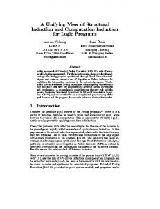
2.1 Equations of Motion The process of a sphere impacting a simply supported plate, as depicted in Fig. 2.1, can be divided into two individual sub-processes with their own particular sets of equations of motion (EOM). The first set describes the free fall of the sphere before and after an impact and the free vibration of the plate after the impact while the second set of EOMs models the impact process between the two bodies.

Figure 2.1: Side view of problem setup. Offset of forces only for visualisation. 𝐹𝑔 denotes the gravitational force, 𝐹𝑐 the contact force. (•) contact point (𝑥𝑐 , 𝑦𝑐 ), (×) location of active force (𝑥𝑎 , 𝑦𝑎 ). For the special case considered here (𝑥𝑐 , 𝑦𝑐 ) = (𝑥𝑎 , 𝑦𝑎 ).

3

2 Theory

For a reference point 𝜉𝑠 at the lowest part of the sphere, the free fall and the subsequent “free rebounds” are given by 1 𝜉𝑠 (𝑡) = − 𝑔𝑡2 + 𝑣𝑠,0 𝑡 + 𝜉𝑠,0 2 𝑣𝑠 (𝑡) = − 𝑔𝑡 + 𝑣𝑠,0

(2.1b)

𝑎𝑠 (𝑡) = − 𝑔 ,

(2.1c)

(2.1a)

with 𝑔 being the gravitational constant, the subscript 0 denoting initial values at the start of the free fall and 𝑣𝑠 and 𝑎𝑠 denoting sphere velocity and acceleration. These equations are straightforward analytically to solve and fully describe the motion of the sphere while it is not in contact with the plate. For the case of contact, as shown in Fig. 2.1, the EOM of the sphere is given by − 𝑚𝑠 𝑔 − 𝑚𝑠

𝜕 2 𝜉𝑠 (𝑡) + 𝐹𝑐 (𝑡) = 0 , 𝜕𝑡2

(2.2)

where 𝑚𝑠 is the mass of the sphere and 𝐹𝑐 denotes the contact force between sphere and plate. As the active force 𝐹𝑎 is defined to act on the plate, it has not to be included in (2.2). The free vibration of the plate is given by the convolution of the exciting forces — in this case 𝐹𝑐 and 𝐹𝑎 — with the corresponding Green’s functions 𝑔𝑐,𝜉 (𝑡) or 𝑔𝑎,𝜉 (𝑡) of the plate:

𝜉𝑝 (𝑡) = −𝐹𝑐 (𝑡) * 𝑔𝑐,𝜉 (𝑡) + 𝐹𝑎 (𝑡) * 𝑔𝑎,𝜉 (𝑡) ∫︁𝑡 ∫︁𝑡 = − 𝐹𝑐 (𝜏 ) 𝑔𝑐,𝜉 (𝑡 − 𝜏 ) 𝑑𝜏 + 𝐹𝑎 (𝜏 ) 𝑔𝑎,𝜉 (𝑡 − 𝜏 ) 𝑑𝜏 . 0

(2.3)

0

For the special case considered here, where the active force acts at the contact location, thus (𝑥𝑐 , 𝑦𝑐 ) = (𝑥𝑎 , 𝑦𝑎 ), (2.3) simplifies to

4

2 Theory

𝜉𝑝 (𝑡) = [−𝐹𝑐 (𝑡) + 𝐹𝑎 (𝑡)] * 𝑔𝑐,𝜉 (𝑡) ∫︁𝑡 = [−𝐹𝑐 (𝜏 ) + 𝐹𝑎 (𝜏 )] · 𝑔𝑐,𝜉 (𝑡 − 𝜏 ) 𝑑𝜏 .

(2.4)

0

The Green’s function is given by an eigenfunction expansion (e.g. see [6]) 𝑔𝑐,𝜉 (𝑡) = − 𝜆

∞ ∑︁ ∞ ∑︁

Φ𝑚,𝑛,𝑒 Φ𝑚,𝑛,𝑟 ·

𝑚=1 𝑛=1

sin(Θ𝑚,𝑛 𝑡) −𝛿𝑚,𝑛 𝑡 ·𝑒 , Θ𝑚,𝑛

(2.5)

with 𝜆=

4 , 𝑚′′ 𝑙𝑥 𝑙𝑦

where 𝑚′′ = 𝜌𝑝 ℎ is the mass per unit area of the plate and 𝑙𝑥 and 𝑙𝑦 are the plate’s dimensions in x- and y-direction. Φ𝑚,𝑛,𝑒 and Φ𝑚,𝑛,𝑟 are the plate’s eigenfunctions at the excitation point (𝑥𝑒 , 𝑦𝑒 ), respectively the arbitrary receiving point (𝑥𝑟 , 𝑦𝑟 ). For a simply supported plate they are given by (︂ Φ𝑚,𝑛,𝑖 = sin

𝑚𝜋𝑥𝑖 𝑙𝑥

)︂

(︂ sin

𝑛𝜋𝑦𝑖 𝑙𝑦

)︂ ,

with

𝑖 = {𝑒, 𝑟} .

(2.6)

Θ𝑚,𝑛 and 𝛿𝑚,𝑛 relate to the eigenfrequencies 𝜔𝑚,𝑛 of the plate and introduce the plate damping into the EOM. They are given by

√︂ Θ𝑚,𝑛 = 𝜔𝑚,𝑛 · 𝛿𝑚,𝑛 =

𝜂 𝜔𝑚,𝑛 , 2

1−

𝜂2 4

(2.7a) (2.7b)

where 𝜂 is the loss factor of the plate which for this study is assumed to be independent of frequency.

5

2 Theory

The eigenfrequencies are given by √︂ 𝜔𝑚,𝑛 =

𝐵′ · 𝑚′′

[︃(︂

𝑚𝜋 𝑙𝑥

)︂2

(︂ +

𝑛𝜋 𝑙𝑦

)︂2 ]︃ ,

(2.8)

with 𝐵 ′ being the bending stiffness of the plate defined as 𝐵′ =

𝐸ℎ3 . 12(1 − 𝜇2𝑝 )

(2.9)

For this study, the excitation as well as receiving point are set to be located at the contact point, hence (𝑥𝑒 , 𝑦𝑒 ) = (𝑥𝑟 , 𝑦𝑟 ) = (𝑥𝑐 , 𝑦𝑐 ) for (2.5) and (2.6). Before the different equations for the sub-parts of the model can be combined to form a single equation for the contact process, a local displacement variable 𝜉 expressing the distance between the lowest point of the sphere 𝜉𝑠 and the plate surface 𝜉𝑝 (see Fig. 2.1) has to be introduced 𝜉(𝑡) = 𝜉𝑠 (𝑡) − 𝜉𝑝 (𝑡) .

(2.10)

For sphere-plate contact it is 𝜉(𝑡) ≤ 0, in this case 𝜉 expresses the penetration depth of the sphere into the plate as shown by Fig. 2.2.

Figure 2.2: Deformation of plate and sphere during contact. Black: actual shape of plate and sphere during contact. Grey: Shape without deformation.

6

2 Theory Moreover, also a relative velocity and acceleration can be defined

𝜕𝜉(𝑡) 𝜕𝑡 𝜕 2 𝜉(𝑡) . 𝜕𝑡2

𝑣(𝑡) := 𝑎(𝑡) :=

(2.11a) (2.11b)

In order to combine the EOMs of the plate and the sphere (2.4) has to be differentiated twice with respect to time:

𝜕2 𝜕2 𝜉 (𝑡) = − 𝑝 𝜕𝑡2 𝜕𝑡2

∫︁𝑡

𝜕2 𝐹𝑐 (𝜏 ) 𝑔𝑐,𝜉 (𝑡 − 𝜏 ) 𝑑𝜏 + 2 𝜕𝑡

0

∫︁𝑡 = −

𝐹𝑐 (𝜏 )

∫︁𝑡 𝐹𝑎 (𝜏 ) 𝑔𝑐,𝜉 (𝑡 − 𝜏 ) 𝑑𝜏 0

𝜕2 𝑔𝑐,𝜉 (𝑡 − 𝜏 ) 𝑑𝜏 + 𝜕𝑡2

∫︁𝑡 𝐹𝑎 (𝜏 )

𝜕2 𝑔𝑐,𝜉 (𝑡 − 𝜏 ) 𝑑𝜏 𝜕𝑡2

0

0

= −𝐹𝑐 (𝑡) * 𝑔𝑐,𝑎 (𝑡) + 𝐹𝑎 (𝑡) * 𝑔𝑐,𝑎 (𝑡) .

(2.12)

Here 𝑔𝑐,𝑎 is the Green’s function for the acceleration of the plate, it is the second derivative of the ordinary Green’s function 𝑔𝑐,𝜉 𝜕2 𝑔𝑐,𝜉 (𝑡) 𝜕𝑡2 ∞ ∑︁ ∞ ∑︁ Φ𝑚,𝑛,𝑒 Φ𝑚,𝑛,𝑟 = −𝜆 Θ𝑚,𝑛 𝑛=1 𝑚=1 [︀ 2 ]︀ · (𝛿𝑚,𝑛 − Θ2𝑚,𝑛 ) sin(Θ𝑚,𝑛 ) − 2𝛿𝑚,𝑛 Θ𝑚,𝑛 cos(Θ𝑚,𝑛 ) 𝑒−𝛿𝑚,𝑛 𝑡 .

𝑔𝑐,𝑎 (𝑡) =

(2.13)

Now the EOMs can be combined by multiplying (2.12) by 𝑚𝑠 and adding it to (2.2). Together with (2.10) this yields

−𝑚𝑠 𝑔 − 𝑚𝑠

𝜕 2 𝜉(𝑡) + 𝐹𝑐 (𝑡) = − 𝑚𝑠 𝐹𝑐 (𝑡) * 𝑔𝑐,𝑎 (𝑡) + 𝑚𝑠 𝐹𝑎 (𝑡) * 𝑔𝑐,𝑎 (𝑡) . 𝜕𝑡2

(2.14)

Substitution with (2.11b) finally gives −𝑚𝑠 𝑔 − 𝑚𝑠 𝑎(𝑡) + 𝐹𝑐 (𝑡) = − 𝑚𝑠 𝐹𝑐 (𝑡) * 𝑔𝑐,𝑎 (𝑡) + 𝑚𝑠 𝐹𝑎 (𝑡) * 𝑔𝑐,𝑎 (𝑡) .

7

(2.15)

2 Theory

2.2 The Hertzian Contact In this study the Hertz theory of elastic contact (e.g. see [7] and [8]) is used to describe the contact force 𝐹𝑐 . Generally, 𝐹𝑐 could simply be modelled by Hooke’s law as an ordinary spring force 𝐹 = 𝑠𝑥. This, however, would neglect some important effects. These are mostly caused by the curved surface of the sphere and include the change of contact surface and local deformations of both bodies during the impact. The Hertz law of contact takes account of these effects and defines a non-linear contact force 3

𝐹𝑐 (𝑡) = 𝑠 𝜉(𝑡) 2 .

(2.16)

𝑠 is the contact stiffness 𝑠=

𝐸𝑠′ 𝐸𝑝′ 4√ 𝑅· ′ , 3 𝐸𝑠 + 𝐸𝑝′

with

𝐸′ =

𝐸 , 1 − 𝜇2

(2.17)

where 𝑅 is the radius of the sphere and 𝐸𝑠 , 𝜇𝑠 and 𝐸𝑝 , 𝜇𝑝 are the Young’s modulus and Poisson’s ratio of the sphere respectively the plate. Hertz’ theory is based on the assumption [8] that the colliding bodies can both be regarded as elastic half-spaces loaded over a small elliptical region of their plane surfaces. Furthermore, contact strains must be small enough to be covered by the linear theory of elasticity. This implies that the significant dimensions of the contact area must be small when compared with the dimensions of the colliding bodies and their relative radii of curvature. Moreover, the two bodies also have to have identical (or at least similar) elastic properties or the contact has to be frictionless [9]. In spite of all these limitations there are many reports (e.g. [7], [9] or [10]) that Hertz’ theory accurately predicts parameters even for impacts beyond the strict limits of its validity. Nevertheless, according to Goldsmith [7] theory reaches its limits for impacts involving soft materials or high impact velocities. This is, however, not surprising as these conditions clearly violate the aforementioned assumptions. For the case considered here Eq. (2.16) has to be modified in two ways: The coordinate system defined in Fig. 2.1 has to be taken into account and a Heaviside step function has to be introduced in order to consider that 𝐹𝑐 only acts when the plate and the sphere are in contact. This finally yields 3

𝐹𝑐 (𝑡) = 𝑠 (−𝜉(𝑡)) 2 ℋ{−𝜉(𝑡)} ,

8

(2.18)

2 Theory

with the Heaviside step function being defined as ⎧ ⎨0 for −𝜉(𝑡) < 0 , ℋ{−𝜉(𝑡)} = ⎩1 for −𝜉(𝑡) ≥ 0 .

(2.19)

The Hertz theory of elastic contact also provides information about the impact duration. According to [11] the contact time for the Hertz theory is given as 𝑇𝐻 = 3.214 ·

(︁ 𝑚 )︁ 2 𝑠

𝑠

5

− 15

· 𝑣0

.

(2.20)

Strictly speaking (2.20) is only valid for the classical Hertzian contact involving a plate with semi-infinite thickness. For thin plates the contact time is found (see [12, 13]) to be 𝑇𝑚 = 0.311 · 𝑇𝐻

(2.21)

for plates where reflections from the boundaries reach the contact point after the impact has finished.

2.3 Relaxation In order to better account for the energy loss during the impact, a relaxation model is introduced to provide a physically reasonable description of this damping [5, 8]. While it is obvious that there are a lot more processes of energy loss involved in the impact step than only relaxation, e.g. dissipation due to friction, inelastic deformation or compression of air, it has to be noted that the topic of impact energy loss is complex and still a field of ongoing research ([10] or [14]). Within the scope of this study it is decided to use a relaxation model as one way of introducing damping into the numerical simulations. The idea behind the relaxation model is that the acting force not only depends on the actual deformation, but also on all previous deformations, i.e. it is assumed that some kind of the deformation history exists to which the material adjusts. This adjustment leads to a certain amount of energy dissipation. In [15] relaxation according to Boltzmann is defined as

9

2 Theory

∫︁∞ 𝜎(𝑡) = 𝐷𝜖(𝑡) −

𝜖(𝑡 − ∆𝑡) 𝜙(∆𝑡) 𝑑(∆𝑡) ,

(2.22)

0

where the stress 𝜎 and the strain 𝜖 are not only related by the modulus of elasticity 𝐷 but also using the mentioned approach involving their previous history. This is done by integration of the term including the after-effect function 𝜙(∆𝑡) which in this case is given by 𝜙(∆𝑡) =

𝐷𝜏 − Δ𝑡 𝑒 𝜏 . 𝜏

(2.23)

Introducing (2.22) and (2.23) into the equation for the Hertzian contact force (2.18) yields

⎡

∫︁𝑡

𝐹𝑐,𝜏 (𝑡) = ⎣𝑠𝑟𝑒𝑙 (−𝜉(𝑡)) −

⎤

(−𝜉(𝑡 − ∆𝑡))

𝑠𝜏 − Δ𝑡 𝑒 𝜏 𝑑(∆𝑡)⎦ 𝜏

0

√︀ · −𝜉(𝑡) · ℋ{−𝜉(𝑡)} )︁]︁ √︀ [︁ 𝑡 𝑠𝜏 (︁ (−𝜉(𝑡)) * 𝑒− 𝜏 −𝜉(𝑡) · ℋ{−𝜉(𝑡)} . = 𝑠𝑟𝑒𝑙 (−𝜉(𝑡)) − 𝜏

(2.24a) (2.24b)

According to [5], only the linear part of (2.18) is replaced as the non-linear part is only related to the change of the contact area during the course of the impact. Relaxation, however, can only replace the linear part as it only depends on material properties and not the contact area. 𝑠𝑟𝑒𝑙 and 𝑠𝜏 are the modified contact stiffnesses for the relaxation model. Replacing 𝐹𝑐 in (2.15) with 𝐹𝑐,𝜏 finally gives the complete analytical description of the contact between sphere and plate [︁ )︁]︁ √︀ 𝑡 𝑠𝜏 (︁ −𝑚𝑠 𝑔 − 𝑚𝑠 𝑎(𝑡)+ 𝑠𝑟𝑒𝑙 (−𝜉(𝑡)) − (−𝜉(𝑡)) * 𝑒− 𝜏 −𝜉(𝑡) · ℋ{−𝜉(𝑡)} 𝜏 (︁ [︁ )︁]︁ √︀ 𝑡 𝑠𝜏 = −𝑚𝑠 𝑔𝑐,𝑎 (𝑡)* 𝑠𝑟𝑒𝑙 (−𝜉(𝑡)) − (−𝜉(𝑡)) * 𝑒− 𝜏 −𝜉(𝑡) · ℋ{−𝜉(𝑡)} 𝜏 +𝑚𝑠 𝐹𝑎 (𝑡)*𝑔𝑐,𝑎 (𝑡) .

10

(2.25)

2 Theory Regarding the use of relaxation as a means of introducing damping into the impact simulation it has to be noted that this is only one of several techniques proposed in literature (for an overview see e.g. [16]). Like the relaxation model, these techniques utilise only one mechanism to describe the manifold damping processes during the impact. Hence, they also share the relaxation model’s shortcoming of being an auxiliary construct rather than a full physical description of the involved processes. Due to the inherent differences of introducing damping between the various models it is deemed necessary to also evaluate a second technique. This is done in Sec. 2.6 where a linear viscous damping model is discussed. The goal is to find the model which yields best efficiency, ease of use and, most important, provides the best conditions for the introduction of the active force. For the sake of clarity the derivation of the necessary equations for the simulation is at first continued solely for the relaxation model. After this is fully implemented, the necessary changes for a linear viscous damping model are described in Sec. 2.6.

2.4 Discretisation As it is difficult, if not impossible, to analytically solve the non-linear ordinary differential equation (ODE) (2.25), a numerical approach has to be taken to determine the solution of the contact equation. The first step in the discretisation of (2.25) is omitting the Heaviside step function ℋ{−𝜉(𝑡)}. This can be done under the assumption that the numerical representation of (2.25) will only be calculated while the sphere and the plate actually are in contact. For the other times it is much more efficient and straightforward to calculate sphere and plate movement individually using equations (2.1a) to (2.1c) respectively (2.4). The next step is the discretisation of the convolutions. According to [17] the timediscrete convolution of two functions 𝑓 (𝑡) and 𝑔(𝑡) at time step 𝑁 is given by (𝑓 * 𝑔)(𝑡𝑁 ) = ∆𝑡

𝑁 ∑︁

𝑓 (𝑡𝑖 ) 𝑔(𝑡𝑁 −𝑖+1 ) ,

(2.26)

𝑖=1

with ∆𝑡 being the size of the discretisation steps. It now has to be kept in mind, that — assuming 𝑓 (𝑡) represents 𝜉(𝑡) — in (2.25) a solution for 𝜉(𝑡) is sought. In the discretised form of the equation, which has to be solved individually for every time step, it is thus required to have full access to all occurrences of 𝜉(𝑡𝑁 ), including those involved in convolutions. This is achieved by removing the

11

2 Theory present time step 𝑁 with the unknown 𝑓 (𝑡𝑁 ) (or 𝜉(𝑡𝑁 )) out of the convolution sum, which then only includes known quantities as it represents all previous time steps: ∆𝑡

𝑁 ∑︁

𝑓 (𝑡𝑖 )𝑔(𝑡𝑁 −𝑖+1 ) = ∆𝑡 𝑓 (𝑡𝑁 )𝑔(𝑡1 ) + ∆𝑡

𝑖=1

𝑁 −1 ∑︁

𝑓 (𝑡𝑖 )𝑔(𝑡𝑁 −𝑖+1 ) .

(2.27)

𝑖=1

Applying (2.26) and (2.27) to (2.25), while omitting ℋ{−𝜉(𝑡)}, yields

− 𝑚𝑠 𝑔 − 𝑚𝑠 𝑎(𝑡𝑁 )+ [︃

]︃ 𝑁 −1 ∑︁ 𝑡𝑁 −𝑖+1 √︀ 𝑡1 𝑠𝜏 −𝜉(𝑡𝑁 ) (−𝜉(𝑡𝑖 )) 𝑒− 𝜏 ) 𝑠𝑟𝑒𝑙 (−𝜉(𝑡𝑁 )) − ∆𝑡 (−𝜉(𝑡𝑁 ))𝑒− 𝜏 − 𝜏 𝑖=1 (︃ ]︃)︃ [︃ 𝑁 −1 ∑︁ 𝑡𝑁 −𝑖+1 √︀ 𝑡1 𝑠𝜏 = −𝑚𝑠 ∆𝑡·𝑔𝑐,𝑎 (𝑡1 )· −𝜉(𝑡𝑁 ) 𝑠𝑟𝑒𝑙 (−𝜉(𝑡𝑁 )) − ∆𝑡 (−𝜉(𝑡𝑁 ))𝑒− 𝜏 + (−𝜉(𝑡𝑖 )) 𝑒− 𝜏 𝜏 𝑖=1 ⎛ ⎡ ⎤⎞ 𝑁 −1 𝑖 ∑︁ ∑︁ 𝑡 √︀ 𝑗−𝑖+1 𝑠𝜏 −𝑚𝑠 ∆𝑡 ⎝ 𝑔𝑐,𝑎 (𝑡𝑁 −𝑖+1 ) · −𝜉(𝑡𝑖 ) · ⎣𝑠𝑟𝑒𝑙 (−𝜉(𝑡𝑖 )) − ∆𝑡 (−𝜉(𝑡𝑗 ))𝑒− 𝜏 ⎦⎠ 𝜏 𝑖=1

𝑗=1

+ 𝑚𝑠 ∆𝑡

𝑁 ∑︁

𝐹𝑎 (𝑡𝑖 ) · 𝑔𝑐,𝑎 (𝑡𝑁 −𝑖+1 ) . (2.28)

𝑖=1

Substituting the parts for the previous time steps with

𝑁 −1 𝑡𝑁 −𝑖+1 𝑠𝜏 ∑︁ Ξ(𝑡𝑁 ) =∆𝑡 (−𝜉(𝑡𝑖 )) 𝑒− 𝜏 𝜏 𝑖=1 𝑁 −1 ∑︁

Π(𝑡𝑁 ) =𝑚𝑠 ∆𝑡 ·

𝑔𝑐,𝑎 (𝑡𝑁 −𝑖+1 ) ·

(2.29a)

√︀ −𝜉(𝑡𝑖 )

𝑖=1

⎡

⎤ 𝑖 ∑︁ 𝑡 𝑗−𝑖+1 𝑠𝜏 · ⎣𝑠𝑟𝑒𝑙 (−𝜉(𝑡𝑖 )) − ∆𝑡 (−𝜉(𝑡𝑗 ))𝑒− 𝜏 ⎦ 𝜏

(2.29b)

𝑗=1

(2.29c) and the convolution of 𝐹𝑎 and 𝑔𝑐,𝑎 with

𝐴1 (𝑡𝑁 ) =𝑚𝑠 ∆𝑡

𝑁 ∑︁

𝐹𝑎 (𝑡𝑖 ) · 𝑔𝑐,𝑎 (𝑡𝑁 −𝑖+1 )

𝑖=1

12

(2.29d)

2 Theory

gives [︁ ]︁ √︀ 𝑡1 𝑠𝜏 −𝑚𝑠 𝑔−𝑚𝑠 𝑎(𝑡𝑁 ) + 𝑠𝑟𝑒𝑙 (−𝜉(𝑡𝑁 )) − ∆𝑡 (−𝜉(𝑡𝑁 ))𝑒− 𝜏 − Ξ(𝑡𝑁 ) −𝜉(𝑡𝑁 ) 𝜏(︁ )︁ √︀ 𝑡1 𝑠𝜏 = − 𝑚𝑠 ∆𝑡 · 𝑔𝑐,𝑎 (𝑡1 ) · −𝜉(𝑡𝑁 ) 𝑠𝑟𝑒𝑙 (−𝜉(𝑡𝑁 )) − ∆𝑡 (−𝜉(𝑡𝑁 ))𝑒− 𝜏 − Ξ(𝑡𝑁 ) 𝜏 − Π(𝑡𝑁 ) + 𝐴1 (𝑡𝑁 ) . (2.30) Simplifying finally yields

0 = 𝑚𝑠 𝑔 + 𝑚𝑠 𝑎(𝑡𝑁 ) −

[︁ ]︁ √︀ 𝑡1 𝑠𝜏 −𝜉(𝑡𝑁 ) (−𝜉(𝑡𝑁 ))(𝑠𝑟𝑒𝑙 − ∆𝑡 𝑒− 𝜏 ) − Ξ(𝑡𝑁 ) 𝜏 · [1 + 𝑚𝑠 ∆𝑡 · 𝑔𝑐,𝑎 (𝑡1 )] − Π(𝑡𝑁 ) + 𝐴1 (𝑡𝑁 ) . (2.31)

Eq. (2.31), however, still includes two unknown variables, namely 𝑎(𝑡𝑁 ) and 𝜉(𝑡𝑁 ). These can be related numerically using the Newmark (NM) or the Hilber-Hughes-Taylor (HHT) methods, both of which make use of the dependence between 𝜉(𝑡𝑁 ), 𝑣(𝑡𝑁 ) and 𝑎(𝑡𝑁 ) and the knowledge about the corresponding values at the preceding time step 𝑁 − 1. The NM is defined as [17]

𝑣𝑁 𝑀 (𝑡𝑁 ) = 𝑣(𝑡𝑁 −1 ) + ∆𝑡[(1 − 𝛾) 𝑎(𝑡𝑁 −1 ) + 𝛾𝑎(𝑡𝑁 )] (2.32a) )︂ ]︂ [︂(︂ 1 − 𝛽 𝑎(𝑡𝑁 −1 ) + 𝛽𝑎(𝑡𝑁 ) .(2.32b) 𝜉𝑁 𝑀 (𝑡𝑁 ) = 𝜉(𝑡𝑁 −1 ) + ∆𝑡𝑣(𝑡𝑁 −1 ) + ∆𝑡2 2

Usually 𝛾 and 𝛽 are chosen such that 𝛾 =

1 2

and 𝛽 =

1 4,

leading to an implicit

trapezoidal method which is A-stable and of second order accuracy [18]. The drawback of the Newmark method is its lack of numerical damping which makes it prone to parasitic high-frequency oscillations induced by the discretisation process. The HHT method is an enhancement of the Newmark method which preserves the numerical properties while introducing some level of numerical damping. It is defined as [19]

13

2 Theory

𝑣𝐻𝐻𝑇 (𝑡𝑁 ) = (1 + 𝛼)𝑣(𝑡𝑁 −1 ) − 𝛼𝑣𝑁 𝑀 (𝑡𝑁 ) = 𝑣(𝑡𝑁 −1 ) − 𝛼∆𝑡 [(1 − 𝛾) 𝑎(𝑡𝑁 −1 ) + 𝛾 𝑎(𝑡𝑁 )]

(2.33a)

𝜉𝐻𝐻𝑇 (𝑡𝑁 ) = (1 + 𝛼)𝜉(𝑡𝑁 −1 ) − 𝛼𝜉𝑁 𝑀 (𝑡𝑁 ) = 𝜉(𝑡𝑁 −1 ) − 𝛼∆𝑡 𝑣(𝑡𝑁 −1 ) 1 −𝛼∆𝑡2 [( − 𝛽) 𝑎(𝑡𝑁 −1 ) + 𝛽𝑎(𝑡𝑁 )] , 2

(2.33b)

with

1 − 2𝛼 2

𝛾=

𝛽=

(1 − 𝛼)2 4

(2.34)

and values of 𝛼 in the range [− 31 , 0], with smaller values representing higher damping. Replacing 𝜉(𝑡𝑁 ) in (2.31) with 𝜉𝐻𝐻𝑇 (𝑡𝑁 ) finally yields

1 (︀ )︀ 𝑓𝑁 𝑤𝑡 = 𝑚𝑠 𝑔 + 𝑚𝑠 𝑎(𝑡𝑁 ) − 𝐴22 (𝑡𝑁 ) · 𝐴2 (𝑡𝑁 ) · 𝐵1 − Ξ(𝑡𝑁 ) · 𝐵2

−Π(𝑡𝑁 ) + 𝐴1 (𝑡𝑁 ) = 0.

(2.35)

with 𝐴2 (𝑡𝑁 ) = −𝜉(𝑡𝑁 −1 ) + 𝛼∆𝑡 𝑣(𝑡𝑁 −1 ) [︂(︂ )︂ ]︂ 1 2 +𝛼∆𝑡 − 𝛽 𝑎(𝑡𝑁 −1 ) + 𝛽𝑎(𝑡𝑁 ) 2 𝑡1 𝑠𝜏 𝐵1 = 𝑠𝑟𝑒𝑙 − ∆𝑡 𝑒− 𝜏 𝜏 𝐵2 = 1 + 𝑚𝑠 ∆𝑡 · 𝑔𝑐,𝑎 (𝑡1 ) .

(2.36a) (2.36b) (2.36c)

In Eq. (2.35) 𝑎(𝑡𝑁 ) remains the only unknown. For solving the numerical NewtonRaphson algorithm (see e.g. [20] or [21]) is employed, which iteratively calculates the root of 𝑓𝑁 𝑤𝑡 and is known to provide fast (actual quadratical) convergence. For the present case it is given as 𝑎(𝑡𝑁,𝑖 ) = 𝑎(𝑡𝑁,𝑖−1 ) −

14

𝑓𝑁 𝑤𝑡 , 𝜕𝑓𝑁 𝑤𝑡 /𝜕𝑎(𝑡𝑁 )

(2.37)

2 Theory

with 𝑖 being the iteration number. The break-off condition is |𝑎(𝑡𝑁,𝑖 ) − 𝑎(𝑡𝑁,𝑖−1 )| < 𝜖, i.e. the root is assumed to be found when the results of two consecutive iterations do not differ by more than a maximum error of 𝜖, which here is set to be 𝜖 = ∆𝑡. The missing derivative of 𝑓𝑁 𝑤𝑡 (Eq. (2.35)) with respect to 𝑎(𝑡𝑁 ) is

(︀ )︀ 1 𝜕𝑓𝑁 𝑤𝑡 1 −1 = 𝑚𝑠 − 𝐴2 2 (𝑡𝑁 ) · [𝛼∆𝑡2 𝛽] 2 · 𝐴2 (𝑡𝑁 ) · 𝐵1 − Ξ(𝑡𝑁 ) · 𝐵2 𝜕𝑎(𝑡𝑁 ) 2 1

−𝐴22 (𝑡𝑁 ) · (𝛼∆𝑡2 𝛽𝐵1 ) · 𝐵2 .

(2.38)

Hereby, the numerical description of the impact process is complete. Starting with initial values for 𝜉(𝑡𝑁 −1 ), 𝑣(𝑡𝑁 −1 ) and 𝑎(𝑡𝑁 −1 ), which are either given by the free fall (cf. (2.1a) to (2.1c)) for the first impact step or by the preceding step for all following steps, 𝑎(𝑡𝑁 ) can be calculated using (2.37) followed by calculation of 𝑣(𝑡𝑁 ) and 𝜉(𝑡𝑁 ) using the Hilber-Hughes-Taylor equations (2.33). This is repeated until the sphere and the plate separate again, i.e. 𝜉(𝑡𝑁 ) > 0. Now the next free fall starts (with the last numerically calculated 𝜉(𝑡𝑁 ) and 𝑣(𝑡𝑁 ) as starting values) and the plate vibrates freely. A flowchart representation of the numerical impact calculations is given in Fig. 2.3. The vibration of the plate can be calculated by the time discrete version of (2.4)

𝜉𝑝 (𝑡𝑁 ) = −∆𝑡

𝑁 ∑︁

𝐹𝑐,𝜏 (𝑡𝑖 ) · 𝑔𝑐,𝜉 (𝑡𝑁 −𝑖+1 ) + ∆𝑡

𝑖=1

𝑁 ∑︁

𝐹𝑎 (𝑡𝑖 ) · 𝑔𝑐,𝜉 (𝑡𝑁 −𝑖+1 ) ,

(2.39)

𝑖=1

where the discrete version of the contact force is given as ⎡

⎤ 𝑖 ∑︁ 𝑡𝑗−𝑖+1 √︀ 𝑠 𝜏 𝐹𝑐,𝜏 (𝑡𝑁 ) = ⎣𝑠𝑟𝑒𝑙 (−𝜉(𝑡𝑖 )) − ∆𝑡 (−𝜉(𝑡𝑗 ))𝑒− 𝜏 ⎦ · −𝜉(𝑡𝑖 )) . 𝜏

(2.40)

𝑗=1

This is done separately after each impact for a time-frame ranging from the start of the impact until the end of the simulation. The overall vibration of the plate is then given as the superposition of the individual vibrations for each impact, where obviously for a given time step only present or past impacts are considered. The plate’s velocity 𝑣𝑝 (𝑡𝑁 ) can be calculated in the same way using the Green’s function for velocity 𝑔𝑐,𝑣 .

15

2 Theory

Figure 2.3: Flowchart of numerical impact calculations.

16

2 Theory

2.5 Parameter Estimation for the Relaxation Model In order to properly simulate the impact process information about the relaxation parameters 𝑠𝑟𝑒𝑙 , 𝑠𝜏 and 𝜏 (see (2.24b)) is necessary. Exact specification of these values is difficult as they do not only depend on material properties, but also on the manufacturing process, the age of the workpiece as well as all previous loads. As described in Sec. 2.3, relaxation is included out of the necessity to introduce some sort of reasonable damping into the simulation. While fulfilling this goal, relaxation does not provide a complete picture of the physics of the numerous underlying damping processes. Because of this, it seems feasible that the necessary parameters can be roughly approximated based on knowledge about plate and sphere characteristics. In this regard the coefficient of restitution 𝑐𝑜𝑟 is a helpful quantity. For sphere-plate impacts it is commonly (e.g. see [11]) defined as the ratio of the sphere velocity (or maximum height) before (denoted by 0) and after (denoted by 1) the impact

𝑣𝑠,1 𝑐𝑜𝑟 = = 𝑣𝑠,0

√︃

𝜉𝑠,1 . 𝜉𝑠,0

(2.41)

Energy-wise this can be expressed as 𝐸1 = 𝐸0 𝑐𝑜𝑟2

(2.42)

𝐸𝜂 = 𝐸0 (1 − 𝑐𝑜𝑟2 ) .

(2.43)

or regarding energy loss as

Hence, much like the introduced relaxation model, the coefficient of restitution is a global measure of the energy loss during impact and does not give insight into the different underlying processes. Nevertheless, its simplicity makes it a valuable tool for the evaluation of impacts. In this study it is used to help determine some of the relaxation parameters. The coefficient of restitution assesses the amount of kinetic energy which the sphere can recover from the impact. Accordingly an impact loss factor can be defined to assess the amount of energy lost during the contact 𝜂𝑐 = (1 − 𝑐𝑜𝑟2 ) .

17

(2.44)

2 Theory

The idea is now to find values for 𝑠𝑟𝑒𝑙 , 𝑠𝜏 and 𝜏 which lead to an energy loss during the impact which is similar to values obtained for 𝜂𝑐 using coefficients of restitution available in literature sources such as [7, 10, 11]. In order to do so, one has to start with the contact force at the first time step. As there is no previous deformation history, the force at that moment (2.24b) is equal to the contact force without relaxation (2.18)

⇐⇒

𝐹𝑐 (𝑡1 ) = 𝐹𝑐,𝜏 (𝑡1 ) [︁ ]︁ 𝑡1 3 𝑠𝜏 𝑠 (−𝜉(𝑡1 )) 2 = 𝑠𝑟𝑒𝑙 (−𝜉(𝑡1 )) − ∆𝑡 (−𝜉(𝑡1 ))𝑒− 𝜏 − Ξ(𝑡1 ) 𝜏 √︀ · −𝜉(𝑡1 ) .

(2.45)

For the first step of the impact there is no previous force history, so obviously Ξ(𝑡1 ) = 0. Using 𝑡1 = ∆𝑡 and assuming 𝜏 ≫ ∆𝑡, it is 𝑒−

Δ𝑡 𝜏

≈ 1 in (2.45), which gives

∆𝑡 𝑠𝜏 𝜏 ∆𝑡 = 𝑠− 𝑠𝜏 . 𝜏

𝑠 = 𝑠𝑟𝑒𝑙 − ⇐⇒ 𝑠𝑟𝑒𝑙

(2.46)

This still leaves the two unknowns 𝜏 and 𝑠𝜏 . In [15] the relationship between the (frequency-dependent) loss factor and the relaxation parameters for the Boltzmann model is given as 𝜂=

𝑠𝜏 𝜔𝜏 . 𝑠𝑟𝑒𝑙 − 𝑠𝜏 + 𝑠𝑟𝑒𝑙 𝜔 2 𝜏 2

(2.47)

Strictly speaking Eq. (2.46) is not valid for the case considered here as it is originally used to describe harmonic processes with an angular frequency 𝜔. However, as the whole relaxation model is used somewhat outside its original scope1 , Eq. (2.47) might as well be adapted for the present case. Introducing an angular contact frequency based on the half-cycle contact time 𝑇 𝜔𝑇 = 1

𝜋 𝑇

(2.48)

This is an intrinsic problem of most ways of introducing damping into impact simulations, e.g. it is also the case with a viscous damping model.

18

2 Theory

as a replacement for 𝜔 in (2.47) and assuming that the contact loss factor 𝜂𝑐 can be replaced by (2.44), one finally obtains by inserting (2.46) in (2.47) 𝑠𝜏 =

𝑠 𝜂𝑐 (𝜏 + 𝜔𝑇2 𝜏 3 ) . 𝜂𝑐 (𝜏 − ∆𝑡 − ∆𝑡 𝜔𝑇2 𝜏 2 ) + 𝜔𝑇 𝜏 2

(2.49)

Using average values given in literature (e.g. see [7, 10, 12, 14]) for the contact time 𝑇 , the still unknown 𝜏 can be used to adjust the relaxation parameters in (2.49) and (2.46) such that the resulting rebound heights resemble what is given by the particular coefficient of restitution.

2.6 Viscous Damping As discussed in Sec. 2.3 there exist several ways of introducing damping into the simulated process. Besides the relaxation model which so far has been used in this study, other possible choices are, for example, linear or non-linear viscous damping models of kind 𝐹𝜈 = 𝑐𝑣 (with 𝑐 being the damping factor) respectively 𝐹𝜈 = 𝛽𝜉 𝛾 𝑣 (where 𝛽 and 𝛾 are damping related constants). Even though it is somewhat difficult to imagine viscous forces in solid bodies, a damping model based on viscous forces is worth investigating due to its simplicity. This is believed to lead to EOMs — at least for linear viscous damping — which cannot only be solved more efficiently but which also are more beneficial for the assessment of effective active forces. On the other hand it has to be seen if a viscous model can provide the same level of accuracy as the physically more perspicuous relaxation model. Because the focus lies on efficiency and simplicity of implementation, the linear model is favoured over the non-linear one. For what follows, a viscous damping force has to be defined: 𝐹𝜈 (𝑡) = 𝑐(𝑡) (−𝑣(𝑡)) ℋ{−𝜉(𝑡)} .

(2.50)

The Heaviside step function ℋ{−𝜉(𝑡)} is again introduced to take account for the fact that the force can only act when plate and sphere are in contact. 𝑐(𝑡) is the viscous damping factor which is defined to be time dependent in order to avoid discontinuities. This is realised by introducing a proportionality of kind 𝑐(𝑡) ∝ −𝜉(𝑡). In order to introduce linear viscous damping into the equations derived in Sections 2.1 to 2.4 the viscous damping force 𝐹𝜈 has to be installed as a second force acting between sphere and plate during impact. Hence, in Fig. 2.1 and Equations (2.2) and (2.3) 𝐹𝑐

19

2 Theory has to be replaced with 𝐹𝑐 + 𝐹𝜈 . Here 𝐹𝑐 is the ordinary Hertz contact force according to (2.18), which obviously this time will not be modified to include relaxation as in (2.24b). For the combined EOM of sphere and plate (cf. (2.15)) this leads to

− 𝑚𝑠 𝑔 − 𝑚𝑠 𝑎(𝑡) + 𝐹𝑐 (𝑡) + 𝐹𝜈 (𝑡) = 𝑚𝑠 [𝐹𝑎 (𝑡) − 𝐹𝑐 (𝑡) − 𝐹𝜈 (𝑡)] * 𝑔𝑐,𝑎 (𝑡) .

(2.51)

or, written in the time-discrete version (replacing (2.28)),

− 𝑚𝑠 𝑔 − 𝑚𝑠 𝑎(𝑡𝑁 ) + 𝐹𝑐 (𝑡𝑁 ) + 𝐹𝜈 (𝑡𝑁 ) = 𝑚𝑠 ∆𝑡

𝑁 ∑︁

[𝐹𝑎 (𝑡𝑖 ) − 𝐹𝑐 (𝑡𝑖 ) − 𝐹𝜈 (𝑡𝑖 )] · 𝑔𝑐,𝑎 (𝑡𝑁 −𝑖+1 ) . (2.52)

𝑖=1

The sum again has to be split into a part for the present time step and a part for all previous time steps, with the latter being given by

Υ(𝑡𝑁 ) = 𝑚𝑠 ∆𝑡

𝑁 −1 ∑︁

[︁

]︁ 3 𝐹𝑎 (𝑡𝑖 ) − 𝑠 (−𝜉(𝑡𝑖 )) 2 + 𝑐(𝑡𝑁 ) 𝑣(𝑡𝑖 ) · 𝑔𝑐,𝑎 (𝑡𝑁 −𝑖+1 ) .

(2.53)

𝑖=1

Introducing Υ(𝑡𝑁 ) into (2.52) and simplification yields

(︁ )︁[︁ ]︁ 3 0 = 𝑚𝑠 𝑔 + 𝑚𝑠 𝑎(𝑡𝑁 ) + 𝑚𝑠 ∆𝑡 𝑔𝑐,𝑎 (𝑡1 ) + 1 𝑐(𝑡𝑁 ) 𝑣(𝑡𝑁 ) − 𝑠 (−𝜉(𝑡𝑁 )) 2 + 𝑚𝑠 ∆𝑡 𝑔𝑐,𝑎 (𝑡1 )𝐹𝑎 (𝑡𝑁 ) + Υ(𝑡𝑁 ) . (2.54) Using the Hilber-Hughes-Taylor relations defined in (2.33) one obtains the following equations for use with the Newton-Raphson algorithm (2.37)

[︁ ]︁ 3 𝑓𝑁 𝑤𝑡 = 𝑚𝑠 𝑔 + 𝑚𝑠 𝑎(𝑡𝑁 ) + 𝐵2 𝑐(𝑡𝑁 ) 𝑣𝐻𝐻𝑇 (𝑡𝑁 ) − 𝑠(−𝜉𝐻𝐻𝑇 (𝑡𝑁 )) 2 +𝑚𝑠 ∆𝑡 𝑔𝑐,𝑎 (𝑡1 )𝐹𝑎 (𝑡𝑁 ) + Υ(𝑡𝑁 ) = 0,

20

(2.55)

2 Theory and [︂ ]︂ 1 𝜕𝑓𝑁 𝑤𝑡,𝜈 3 2 2 = 𝑚𝑠 − 𝐵2 𝑐(𝑡𝑁 )𝛾𝛼∆𝑡 + 𝛼𝛽∆𝑡 𝑠(−𝜉𝐻𝐻𝑇 ) 𝜕𝑎(𝑡𝑁 ) 2

(2.56)

where 𝐵2 is defined by (2.36c). The remaining steps are the same as previously described in Sec. 2.4, with the exception that the time discrete vibration of the plate (cf. (2.39)) is given by 𝜉𝑝 (𝑡𝑁 ) = ∆𝑡

𝑁 ∑︁

[𝐹𝑎 (𝑡𝑖 ) − 𝐹𝑐 (𝑡𝑖 ) − 𝐹𝜈 (𝑡𝑖 )] · 𝑔𝑐,𝜉 (𝑡𝑁 −𝑖+1 ) .

(2.57)

𝑖=1

For the numerical simulations the time dependency of 𝑐(𝑡) is assumed to be 𝑐(𝑡𝑁 ) = −𝑐0 𝜉(𝑡𝑁 −1 ) .

(2.58)

Thus, providing a smooth and continuous fade in and out of 𝐹𝜈 at the beginning and end of the contact. Rough estimations of values for 𝑐0 can be obtained using equations given by Brach [11], which relate the coefficient of restitution with the parameters of a linear viscous damping model

√︀ 𝑐𝑜𝑟 = exp(−𝜋𝜁/ 1 − 𝜁 2 ) ,

(2.59a)

with the damping ratio defined as 𝑐 𝜁= √ . 2 𝑚𝑠

(2.59b)

This leads to √︃ 𝑐=

4𝑚𝑠 , 𝜋 2 /[ln 𝑐𝑜𝑟]2 + 1

(2.59c)

with an effective mass 𝑚𝑠 𝑚′𝑝 𝑚= . 𝑚𝑠 + 𝑚′𝑝

21

(2.59d)

2 Theory These equations are based on a model of two masses connected by a spring and a dashpot and hence cannot be used to determine exact, but only approximate, values for 𝑐 based on given values of 𝑐𝑜𝑟. Especially problematic is the modelling of the plate’s mass, as in the derivation of (2.59) it is assumed that both bodies react globally, i.e. as a whole, to the connecting forces. The real impact, however, is dominated by the local behaviour of the small contact region on the plate. Hence, it is not the mass of the whole plate which is relevant, but rather a local part 𝑚′𝑝 . 𝑚′𝑝 can be assessed using Hertz’ theory. The contact volume between a sphere of radius 𝑅 and a massive plane surface is given as [7] 3 𝑎3 = 𝑅 4

(︂

1 1 + 𝜋𝐸𝑠′ 𝜋𝐸𝑝′

)︂ 𝐹𝑐 (𝑡) .

(2.60)

The magnitude of 𝐹𝑐 (𝑡) can be approximated by a simulation of the impact without viscous damping, i.e. 𝑐 = 0. Given the fact that according to (2.58) a time dependent 𝑐(𝑡) is assumed while the set of equations (2.59) is derived for a constant 𝑐 = 𝑐0 and thus underestimates 𝑐0 for (2.58), it is not deemed necessary to calculate the exact time history of 𝑎3 . Instead 𝑎3 is calculated based on max{𝐹𝑐 (𝑡)|𝑐=0 }. This also accommodates the fact that an assumed local mass influencing the contact surely extends to an area somewhat larger than the actual contact region. In this way the local mass can be approximated as 𝑚′𝑝 ≈ 𝑎3 𝜌𝑝 .

(2.61)

It is obvious that due to several reasons (e.g. uncertainty of local mass, applicability of (2.59) for the present case, use of time-dependent 𝑐(𝑡)) the values obtained for 𝑐0 are by far not exact. Nevertheless during the course of the study values of 𝑐0 obtained by the described techniques proved to be adequate starting values for a manual fine tuning. In most cases the initial deviation from the assumed 𝑐𝑜𝑟 was less than 20 %. This value could certainly be improved by a more exact analysis of Equations (2.59) and (2.60). However, due to the nature of the implemented time dependency of 𝑐(𝑡) it is expected that even with a less approximative analysis still a manual adjustment of 𝑐0 would be needed. Hence, the benefit of a more exact description is limited. The necessary values for 𝑐0 are thus obtained with the described approximations and a following manual fine-tuning.

22

3 Noise and Vibration Mechanisms and Countermeasures In order to asses the possibilities of active control of impacts related noise and vibration, the dominating source mechanisms and the parameters on which they depend, have to be known. Generally, impact processes can be characterised to include several sub-mechanisms which give rise to noise and/or vibrations. A comprehensive overview can be found in [22]. Within the scope of this study it is dealt with the three most general and important mechanisms. These are: 1. Acceleration noise caused by pressure perturbations due to the sudden deceleration and acceleration of the sphere at impact, 2. structural vibrations of the plate due to the impact and 3. ringing noise, i.e. sound radiation due to the structural vibrations of the plate. A detailed description of each mechanism is given in the following sections, along with general investigations for each case on how to reduce noise or vibrations with an active force. Finally, a fourth impact parameter which is only indirectly linked to noise and vibration is also covered. This parameter is the rebound height of the sphere, which has some influence on noise and vibration generating mechanisms in the impacts following the first one.

3.1 Acceleration Noise During impact, the sphere undergoes a sudden change in velocity, from the initial impact velocity 𝑣0 to zero velocity and then to the rebound velocity 𝑣1 . As this happens in the split second of contact between plate and sphere, acceleration is very large and portions of the fluid, i.e. the air, surrounding the sphere are compressed in this process. The energy needed for this compression is thereafter radiated as a short noise pulse and referred to as acceleration noise.

23

3 Noise and Vibration Mechanisms and Countermeasures Longhorn [23] has shown that for a rigid sphere undergoing sudden acceleration from or to halt in a compressible fluid the energy needed for this compression is given by 𝜋𝑅3 𝐸𝐴 = 𝜌0 𝑣02 3

(︂

𝑐𝑡0 𝑅

)︂−2 {︁ }︁ 1 − 𝑒−𝑐𝑡0 /𝑅 [cos (𝑐𝑡0 /𝑅) + sin (𝑐𝑡0 /𝑅)] ,

(3.1)

where 𝑅 is the radius of the sphere, 𝜌0 and 𝑐 are the density and speed of sound of air and 𝑡0 is the duration of the acceleration process. For small values of 𝑐𝑡0 /𝑅 this can be approximated as 𝐸𝐴 →

𝜋𝑅3 1 𝜌0 𝑣02 = 𝑉𝑠 𝜌0 𝑣02 , 3 4

(3.2)

i.e. the kinetic energy of an air bag of half the volume of the sphere travelling with speed 𝑣0 . Due to the rebound of the sphere two separate acceleration processes occur, for which, because of the short impact duration, the total energy radiated as acceleration noise is approximately given as the sum of the individual energies [22] 𝐸𝐴,𝑡𝑜𝑡 ≈

𝜋𝑅3 𝜌0 (𝑣02 + 𝑣12 ) . 3

(3.3)

This leaves the impact and rebound speeds 𝑣0 and 𝑣1 as possible parameters for active control. Holmes [24] uses a slightly different expression for the radiated energy of slow impacts1 between bodies of arbitrary shape 𝐸𝐴 =

𝜌0 𝐿3 𝑣02

(︂

𝐿 𝑐𝑡0

)︂5 ,

(3.4)

where 𝐿 is the typical dimension of the bodies. Eq. (3.4) is not strictly valid for the present case, as it deals with impacts between bodies of similar size and shape. Nevertheless it still should give a rough impression of the variables dominating the amount of radiated energy in the impact between sphere and plate. Obviously, the radiated energy reduces for longer contact times, for which there is less sudden compression of the surrounding fluid. Besides the radiated energy also the peak pressure of the radiated noise pulse is of interest. Following [25] an upper bound for the peak pressure 𝑝ˆ(𝑟) obtained in a collision 1

Within the scope of Holmes’ report the cases considered in this study are slow.

24


Figure 3.1: Upper bound of normalised peak pressure as function of normalised contact time.

between spheres is given as

𝑝ˆ𝑢𝑝𝑝𝑒𝑟 (𝑟) ≈

(︁

1.32 + 2𝛿 2 2𝛿 2/3 2𝑟(4𝛿 4 + 1)

𝜌0 𝑐𝑅𝑣0

)︁ .

(3.5)

Herein, 𝑟 is the distance from the impact location and 𝛿 = (𝑐𝑡0 )/(𝜋𝑅) the nondimensional contact time. A graphical representation of Eq. (3.5) is given in Fig. 3.1. Similar to the radiated energy in Eq. (3.4) which decreases with increasing 𝑐𝑡0 /𝐿 the upper bound for the peak pressure decreases with higher values of 𝛿. As neither 𝑐, 𝜌0 𝑅 or 𝐿 can be actively influenced within the scope of this study, the contact time 𝑡0 remains the only alternative besides 𝑣0 for influencing acceleration noise by use of active structural control. For lowering the acceleration noise one thus has to decrease the impact and rebound velocities or extend the contact time between sphere and plate. Direct reduction of the impact speed 𝑣0 , especially for the very first impact, seems very difficult if not impossible. Influence of rebound velocity 𝑣1 on the other hand seems to be feasible. This should not only reduce the radiated energy according to Eq. (3.3) but also decreases the impact velocity for the following impact. This topic will be covered more thoroughly in Sec. 3.4. Nevertheless, taking Equations (3.4) and (3.5) into account, the most promising means of reducing acceleration noise seems to be the extension of the contact time 𝑡0 . In

25

3 Noise and Vibration Mechanisms and Countermeasures this regard it has to be kept in mind that for longer contact times the approximated Equations (3.2) and (3.3) might no longer be valid. As a final note it shall be pointed out that none of the equations in this section gives an exact description of acceleration noise caused by a sphere impacting on and rebounding off a plate. All equations are merely used to approximately assess which parameters are the most important ones for the strength of the acceleration noise.

3.2 Plate Vibrations During the impact, energy is transmitted from the sphere into the plate, where it leads to structural vibrations. The amount of transferred energy is given by

∫︁𝑇 𝐸𝑣𝑖𝑏 =

𝐹 (𝑡) 𝑣𝑝 (𝑡) 𝑑𝑡

(3.6a)

0

or, using a Riemann sum to obtain the time-discrete representation,

𝐸𝑣𝑖𝑏 =

𝑁0 ∑︁

𝐹 (𝑡𝑖 ) 𝑣𝑝 (𝑡𝑖 ) ∆𝑡

(3.6b)

𝑖=1

where 𝑁0 is the number of time steps ∆𝑡 during the period of contact, hence 𝑇 = 𝑁0 ∆𝑡. 𝑣𝑝 expresses the velocity of plate vibrations which can either be obtained from the plate’s displacement 𝑢𝑝 (𝑡)

ℱ

−→

𝑈𝑝 (𝜔)

·𝑗𝜔

−→

𝑉𝑝 (𝜔)

ℱ −1

−→

𝑣𝑝 (𝑡) ,

or, similar to Equations (2.3) and (2.12), by the convolution of the exciting force 𝐹 with the corresponding Green’s function for velocity 𝑔𝑐,𝑣 , which leads to

∫︁𝑇 𝐸𝑣𝑖𝑏 =

𝐹 (𝑡)2 * 𝑔𝑐,𝑣 (𝑡) 𝑑𝑡

0

26

(3.7a)

3 Noise and Vibration Mechanisms and Countermeasures respectively 𝐸𝑣𝑖𝑏 =∆𝑡2

𝑁0 ∑︁ 𝑖 ∑︁

𝐹 (𝑡𝑖 )2 𝑔𝑐,𝑣 (𝑡𝑖−𝑗+1 ) .

(3.7b)

𝑖=1 𝑗=1

In the frequency-domain, this can be expressed as ∫︁∞ 𝐸𝑣𝑖𝑏 =

|𝐹 (𝜔)|2 Re {𝑌𝑠𝑦𝑠 (𝜔)} 𝑑𝜔 . 𝜋

(3.8a)

0

or, as an approximation for short duration impacts with 𝜔 < 1/𝑇 ([15])

𝐸𝑣𝑖𝑏

𝐼2 ≈ 𝐻 𝜋

∫︁∞ Re {𝑌𝑠𝑦𝑠 (𝜔)} 𝑑𝜔 .

(3.8b)

0

Herein, 𝐼𝐻 ≈

√

2𝑚𝑠 𝑣𝑜 and 𝑌𝑠𝑦𝑠 denotes the point mobility of the simplified impact

system consisting of the impacting mass, a mass-less stiffness element and the plate structure. Equations (3.7a) to (3.8a) clearly indicate that the amount of vibrational energy which is transmitted from the sphere to the plate during impact is foremost dependent on the force 𝐹 , which, as is indicated by (3.8b), approximately depends on the impact velocity 𝑣0 . Hence, similar to the findings of Sec. 3.1, the reduction of the impact velocity 𝑣0 is an appropriate, yet difficult to implement, means for the reduction of plate vibrations. Realising that for the case with active structural control at the impact position, 𝐹 is not identical to the contact force −𝐹𝑐 but is given by the sum of all acting forces 𝐹 = −𝐹𝑐 + 𝐹𝑎 − 𝐹𝜈

(3.9)

another possibility for control of plate vibrations arises. Eq. 3.9 reduces the problem of plate vibrations to a classical, excitation force based, problem of active vibration control. However, as plate vibrations are only one part of the process discussed here, it has to be seen what implications an approach based on Eq. (3.9) has for the other parts of the problem, e.g. the ringing noise or the rebound height. Finally, as shown by the integral over contact time in Eq. (3.6a), 𝐸𝑣𝑖𝑏 also depends on the length of the impact 𝑡0 , meaning that for approximately constant forces a reduction of contact time would also lead to a reduction of transmitted energy.

27

3 Noise and Vibration Mechanisms and Countermeasures If it is not the transmitted energy that is of interest, but the maximum level of plate displacement, velocity or acceleration, the corresponding values are again given by convolutions of the exciting force(s) with the respective Green’s function of the plate (cf. Equations (2.3) and (2.12)). Obviously, this results in a dependence on the same parameters as already discussed for the vibrational energy.

3.3 Ringing Noise From a noise control point of view it is not only of interest how much vibrational energy is transferred into the plate during the impact, but also how much is again radiated from the plate as airborne sound. A crucial parameter in this regard is the critical frequency 𝑐 𝑓𝑐 = 2𝜋

√︂

𝑚′′ . 𝐵′

(3.10)

For frequencies below 𝑓𝑐 the coupling between free structural vibrations and the ambient fluid is weak. Hence, radiation from the structure is also limited. For frequencies at and above 𝑓𝑐 there is always one radiation angle for which coupling, and accordingly radiation, is strong. A parameter which gives a quantitative description of the relationship between the structural vibrations and the radiated power is the radiation efficiency [15] 𝜎=

𝑊𝑟𝑎𝑑 1 2 2 𝜌0 𝑐𝑆|𝑣|

.

(3.11)

𝑊𝑟𝑎𝑑 is the power radiated by the structure’s surface 𝑆 which vibrates with the spatially averaged mean-square velocity |𝑣|2 . The denominator describes the power radiated by a piston which has the same surface area and spatially-averaged mean-square velocity as the actual structure. The radiation efficiency is a means of describing how much less — or in some cases, typically around the critical frequency, also how much more — effective the structure radiates in comparison to the idealised case of a moving piston. For most structures it is neither easy to measure nor to analytically describe the radiation efficiency, especially below the critical frequency. However, as it was the case in the previous sections, approximated values are sufficient for an evaluation of the dominant parameters. Fahy [26] gives the following approximations for a rectangular plate of area 𝑆 and perimeter 𝑈

28


⎧ √︂ 𝑓 𝑈 𝑐 ⎪ ⎨ ; 𝑓 ≪ 𝑓𝑐 2𝑓 𝑆 𝜋 𝑓 𝑐 𝑐 𝜎≈ ⎪ ⎩1 ; 𝑓 ≫ 𝑓𝑐 ,

(3.12)

whereas [15, 27, 28] approximate the radiation efficiency 𝜎 for a plate of size 𝑙𝑥 × 𝑙𝑦 √ and frequencies 𝑓 ≥ 𝑐/(4 𝑆) as ⎧ 2 (︂ )︂ 𝑈 𝜆𝑐 ⎪ ⎪ 2 𝑔1 + 𝑔2 ; ⎪ ⎪ ⎨𝑆 𝜆𝑐 √︀ √︀ 𝜎≈ 𝑙𝑥 /𝜆𝑐 + 𝑙𝑦 /𝜆𝑐 ; ⎪ ⎪ {︁ √︀ ⎪ ⎪ ⎩min 1/ 1 − 𝑓𝑐 /𝑓 ;

𝑓 < 𝑓𝑐 𝑓 ≈ 𝑓𝑐 }︁ √︀ √︀ 𝑙𝑥 /𝜆𝑐 + 𝑙𝑦 /𝜆𝑐 ;

(3.13)

𝑓 > 𝑓𝑐 .

Herein 𝑔1 and 𝑔2 are frequency dependent functions given as ⎧ ⎪ ⎨ 4 (1 − 2𝛼2 ) √ 1 ; 𝑓 < 𝑓𝑐 /2 4 𝛼 1 − 𝛼2 𝑔1 = 𝜋 ⎪ ⎩0 ; 𝑓𝑐 /2 < 𝑓 < 𝑓𝑐 ,

(3.14a)

1 (1 − 𝛼2 ) ln[(1 + 𝛼)/(1 − 𝛼)] + 2𝛼 . 4𝜋 4 (1 − 𝛼2 )3/2

(3.14b)

and 𝑔2 =

In (3.13) to (3.14b) 𝜆𝑐 denotes the critical wave length and 𝛼 =

√︀ 𝑓 /𝑓𝑐 . Results

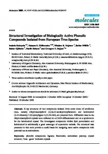
for Equations (3.12) and (3.13) are shown in Fig. 3.2. Obviously, there is a deviation of results for frequencies below 𝑓𝑐 . However, more important than the different low frequency results given by (3.12) and (3.13) is the general tendency for low and high frequency regions. For 𝑓 < 𝑓𝑐 values of 𝜎 are one to two magnitudes lower than for 𝑓 > 𝑓𝑐 , indicating very weak coupling between structural vibrations and radiation to the ambient fluid. For the sake of simplicity and because interest mainly lies on general features, (3.12) will be used for 𝜎 for the remainder of this study. Neither Eq. (3.11), (3.12) nor (3.13) include parameters which could be affected by an active control force to influence radiation efficiency. On the other hand the general characteristics of the radiation efficiency imply another means of minimising ringing noise. Frequencies below 𝑓𝑐 obviously radiate badly, thus it is beneficial to keep the excited frequencies below the critical value. Further on, the excited frequency spectrum

29


30 20

10 logσ

10 0 −10 −20 −30 −2 10

−1

10

0

f /f c

10

1

10

2

10

Figure 3.2: Radiation efficiency for rectangular plate. (—) Eq. (3.13), (−−) Eq. (3.12). depends on the time-history of excitation, i.e. short time-histories with abrupt changes lead to a broadband spectrum going well into high frequency regions whereas longer time histories with only smooth changes limit the spectrum to lower frequency regions. Accordingly, extension of contact time is a viable option for the reduction of ringing noise. This, however, is only partly true if ringing noise is more precisely defined as that part of the radiated sound which lies within the audible frequency range. Assuming that the total amount of radiated energy remains constant, a shortening of the excitation can shift larger portions of the radiated energy into the ultrasonics range, thus reducing the amount of audible ringing noise. Hence, depending on circumstances and seen from a theoretical point of view, either a longer contact time which limits radiation due to small values of radiation efficiency, or a shorter contact time, causing non-audible radiation, can reduce ringing noise. From practical experience, though, it can be argued, that it is usually very difficult to obtain impact conditions which lead to an energy distribution which considerably extends into non-audible frequency regions. Nevertheless, although an extension of contact times seems to be the more appropriate tool, it should be kept in mind that there are two ways of reducing ringing noise by means of change of contact time. Reduction of ringing noise is obviously also achieved by decreasing the overall level of plate vibrations as described in Sec. 3.2. Though reducing |𝑣|2 in Eq. (3.11), this does not significantly affect the value of the radiation efficiency as 𝑊𝑟𝑎𝑑 also reduces when plate vibrations reduce. The amount of energy radiated by the plate as airborne sound is hence controlled by two independent factors: The first being the strength of the structural

30

3 Noise and Vibration Mechanisms and Countermeasures vibrations of the plate itself and the second one being how good these vibrations are radiated as airborne, audible sound. The latter is expressed by the radiation efficiency and the frequency spectrum of the plate vibrations. As a final note it has to be added that for most cases (metal sphere of not too large diameter) radiation due to vibrations of the sphere can be neglected as the even the first eigenfrequency is usually well above the audible range [29].

3.4 Rebound Height Though the rebound height 𝜉𝑟𝑒𝑏 is not a priori linked to any of the noise and vibration generating processes, it is insofar of importance as it plays a significant role for the number of subsequent impacts2 . Obviously, reduction of the number of impacts also implies reduction of the number of vibration and noise generating incidents. Despite the fact that this does not necessarily mean that less vibrational energy will be transferred into the plate, it effectively reduces the total amount of energy radiated as acceleration noise according to Sec. 3.1. Moreover, reduction of rebound height automatically leads to a reduction of the impact velocity 𝑣𝑛𝑒𝑥𝑡 for the following contact. This is beneficial for lowering the peak pressure and overall radiated energy of acceleration noise (cf. Sec. 3.1) and reduces the contact force which governs the strength of plate vibrations (cf. Sec. 3.2) and subsequently the strength of ringing noise (cf. Sec. 3.3). Eq. (2.20) finally shows that reducing the impact velocity also extends the contact time. As pointed out in Sec. 3.3 longer time histories lead to less high frequency content in the spectrum, which can be beneficial regarding the radiation efficiency. The rebound height is given by the EOM of the sphere (2.1a), within which the only parameter being dependent on impact conditions is the initial velocity 𝑣𝑠,0 at the start of the rebound. Accordingly reduction of rebound height can only be achieved by lowering the velocity 𝑣1 with which the sphere leaves the plate at the end of the contact.

3.5 Summary A summary of the conclusions obtained in the previous sections is given in Tab. 3.1. Neglecting interconnection between impact parameters, only direct dependence between contact parameters and noise and vibration mechanisms is shown. This directly leads 2

This, of course, is only true for “free fall” situations and not for machinery like forging hammers or punch presses.

31


Table 3.1: Dependence of noise and vibration mechanisms on impact parameters. For ringing noise only parameters not covered by plate vibrations listed. For all relations only direct dependence included. (↑/↓) Parameter has to be increased/decreased to lower noise or vibrations, (-) no direct influence. acceleration noise 𝑣0 𝑣1 𝐹𝑐 𝑡0

↓ ↓ ↑

To reduce plate vibrations ringing noise ↓ ↓ ↓

↑/↓

rebound height ↓ -

to the major drawback of what so far has been deduced. Most, if not all, of the impact parameters are connected to each other. This means that it is virtually impossible to change one of the quantities without affecting the others. For example changing the contact force (by means of actual vibration control) while maintaining the impact velocity 𝑣0 will definitely influence 𝑡0 and 𝑣1 . As an exact description of the impact is only given by the numerical expressions obtained in Ch. 2, it is not possible to easily assess the exact relationship between the different quantities. Though, it is quite straightforward that a reduction of 𝑣0 will lead to a reduction of 𝑣1 and 𝐹𝑐 while 𝑡0 will extend (see Eq. (2.20)), the exact amount of change is, apart for 𝑡0 , very difficult to quantify before running the numerical simulation. Obviously, this is a consequence of energy conservation between the kinetic energy of the sphere at impact (𝑣0 ), the energy transferred into the plate (𝐹𝑐 , 𝑣𝑝 and 𝑡0 ,) the kinetic energy of the rebound and the amount of energy supplied to the system by the active force. Moreover, the contradicting influence of the contact time depending on the mechanisms under review aggravates the situation. Keeping 𝑡0 low to reduce energy transfer into the plate increases the acceleration noise and leads to high-frequency components in the spectrum which radiate comparably well. Extending the contact time on the other hand means that more of the energy is transferred into the plate. For the ringing noise, finally, extending the contact time seems an appropriate means, however, in special cases reduction can also be achieved by a shortening of the contact. From energy conservation it can generally be concluded that the rebound height, which correlates with one form of potential energy, cannot be influenced without affecting energy transfer to the plate, either in form of local deformation according to the Hertz law or in form of global vibrations of the plate. The same is vice-versa true for reduction

32

3 Noise and Vibration Mechanisms and Countermeasures of plate-vibrations. In any way nearly all of the initial potential energy finally is transferred to the plate. The one exception being the amount of energy dissipated in the various damping processes represented by viscous or relaxation models in this survey. Accordingly, it is physically difficult to obtain a solution which deals equally well with all of the involved mechanisms. Theoretically, an active force configuration has to be found which leads to strong local deformations of sphere and plate — thus lowering the sphere’s energy — without leading to high plate vibrations. Concluding, it can either be aimed for the optimal solution for a specific field of application or for some kind of acceptable combination of broader reduction.

33

4 Evaluation of the Implemented Impact Simulation Before investigating the influence of the active force on the impact process, the implemented numerical simulation of the sphere falling onto the plate as such is investigated. This is done to ensure a correct simulation of the physical process. Furthermore, these investigations are aimed at assessing the applicability of the two employed damping methods for the following studies.

4.1 Simulation Setup The simulations are performed for a simply supported quadratic plate of 0.5 m × 0.5 m as shown by Fig. 4.1. The impact position is exactly in the middle of the plate, i.e. 𝑥𝑖 = 𝑦𝑖 = 0.25 m and the initial drop height is 𝜉𝑠,0 = 0.05 m. The sphere is made out of steel with detailed properties given in Tab. 4.1. The simulations are performed for three different plate materials: Aluminium, oak wood and Getzner Sylomer M [30], a mixed cellular polyurethane used for vibration isolation. A detailed overview of the properties of the different materials can be found in Tab. 4.2. Aluminium and oak are included as examples of widely used plate materials which posses different material properties. The Sylomer M is insofar a special case as it constitutes a comparably soft material which normally is not considered to lead to strong noise or vibration generation during impacts. Moreover, its properties are such, that it

Table 4.1: Overview of sphere properties. 𝑅 radius, 𝐸𝑠 Young’s modulus, 𝜌𝑠 density, 𝜇𝑠 Poisson’s ratio.

Steel

𝑅 in m

𝐸𝑠 in N/m2

𝜌𝑠 in kg/m3

𝜇𝑠 -

0.02

210 · 10+9

7800

0.31

34


Figure 4.1: Top view of problem setup. (•) Impact position, (––) simple support.

is in theory unlikely that all of the assumptions made for the Hertzian contact in Sec. 2.2 are valid. The main reason, why this material is nevertheless included in the study is its comparably low coefficient of restitution. This leads to the assumption that reduction of rebound height can possibly be easily taken to the optimum for this material, i.e. preventing a rebound at all. This extreme case is deemed worth investigation. As stated in Sec. 2.2, the Hertz’ theory is known to give accurate predictions even for impacts outside its strict validity. It is assumed that this is at least also partly true in the Sylomer M case.

Table 4.2: Overview of properties of different plate materials. ℎ plate thickness, 𝐸𝑝 Young’s modulus, 𝜌𝑝 density, 𝜇𝑝 Poisson’s ratio, 𝜂𝑝 loss factor, 𝑐𝑜𝑟 assumed coefficient of restitution for sphere used in this study, 𝑓𝑐 critical frequency.

Aluminium Oak Sylomer M

ℎ in mm

𝐸𝑝 in N/m2

𝜌𝑝 in kg/m3

𝜇𝑝 -

𝜂𝑝 -

𝑐𝑜𝑟 -

𝑓𝑐 Hz

3.0 10.0 12.5

7.2 · 10+10 5 · 10+8 1.34 · 10+6

2700 700 400

0.34 0.10 0.40

1 · 10−4 5 · 10−2 16 · 10−2

0.7 0.6 0.2

3869 7504 80 738

35


1 3

For the HHT algorithm a value of 𝛼 = with a gravitational constant of 𝑔 =

is chosen. All simulations are performed

9.81 m·s−2

and time steps of size ∆𝑡 = 1 · 10−6 s.

According to [15] modal summation for the Green’s functions is performed up to a maximum mode number determined by 𝜔𝑚𝑛,𝑚𝑎𝑥 = 𝜋/∆𝑡. Before an assessment of the simulation results can be conducted, the damping parameters for the relaxation (𝑇 and 𝜏 ) and the viscous damping model (𝑐) have to be adjusted according to Sections 2.5 and 2.6. The obtained values are given in Tab. 4.3. Table 4.3: Obtained damping parameters for given coefficients of restitution. Relaxation 𝑇 𝜏 in s in s Aluminium Oak Sylomer M

21.595 · 10−3 1.027 · 10−3 3.763 65 · 10−3

0.0025 0.5 0.5

Viscous damping 𝑐 12.64175 1.92965 0.107037875

4.2 Comparison of Damping Models Results for both damping models and all plate materials are given in Fig 4.2. Even though parameters of both damping mechanisms are carefully adjusted to give rebound heights nearly perfectly matching the values expected from the coefficients of restitution, there are visible differences between the two models for consecutive rebounds and for the first impact itself. Especially the differences for the impact are interesting considering the fact that for each material the deviation between the first rebound height of the two methods is smaller than 1 · 10−4 m. Hence, even though the impact for the relaxation is longer and more deeply penetrates the plate, the rebound height is nearly exactly the same as for the viscous damping model. This, however, is only true for the first impact(s), for consequent impacts the differences in rebound behaviour are more pronounced. For the later phases of the bouncing, generally relaxation rebound heights are lower. In the case of aluminium and oak this actually leads to a fewer number of rebounds until the sphere lies stationary on the plate. Without extensive experimental evaluation, it is difficult to assess whether one of these simulation models actually is more correct than the other. Nevertheless, keeping in mind that for later rebounds the heights obtained with the viscous damping are closer

36


1

0.025

0

0.02

−1

ξ in m

ξ in m

−6

0.03

0.015

x 10

−2 −3

0.01 −4 0.005 −5 0 0

0.1

0.2

0.3 t in s

0.4

0.5

0.6

0.10096 0.10097 0.10098 0.10099

0.101

0.10101

t in s

(a) Aluminium complete

(b) Aluminium first impact −5

x 10

0.03 0 0.025 −0.5

ξ in m

ξ in m

0.02 0.015 0.01

−1

−1.5

0.005 −2 0 0

0.1

0.2 t in s

0.3

0.4

0.1009

(c) Oak complete

0.101 0.1011 0.1011 0.1012 0.1012 t in s

(d) Oak first impact −5

x 10

0.03 0 0.025 −1 −2 ξ in m

ξ in m

0.02 0.015

−3 −4

0.01 −5 0.005 0 0

−6 −7 0.05

0.1 t in s

0.15

0.2

0.101

(e) Sylomer M complete

0.1012

0.1014 t in s

0.1016

0.1018

(f) Sylomer M first impact

Figure 4.2: Comparison of relaxation and viscous damping simulations. Initial height 0.05 cm at 𝑡 = 0 s. (−−) relaxation, (—) viscous damping, (· · · ) expected rebound heights according to 𝑐𝑜𝑟.

37


Table 4.4: Necessary number of iterations for convergence of Newton-Raphson algorithm. max

min

average

Relaxation


220 649 2 096 352 22 942 400

5 7 4

2853 21 529 18 280

Viscous damping


3 3 3

2 2 2

2 2 2

to those expected from the coefficient of restitution (albeit not matching as perfectly as for the first rebound), it can be argued that the viscous damping model gives a better simulation of the bouncing than the relaxation model. It is possible that the obtained damping values for the relaxation model are only correct for the first impact. As a side note, it shall be added that results for no damping at all (𝑠𝑟𝑒𝑙 = 0 respectively 𝑐 = 0) are exactly identical for both models. Hence, it can be ruled out that differences in software implementation are responsible for the variations. This is not the only downside of the relaxation method, there are two more problematic areas which even more severely affect the usefulness of this damping model for this study. As shown in Tab. 4.4, the Newton-Raphson algorithm (2.37) usually converges to the defined maximum error of 𝜖 = ∆𝑡 within two (and never more than three) iterations for the viscous damping model. For relaxation based damping on the other hand, the number of necessary iterations for convergence is some orders of magnitude higher. Though this severely affects computation time, even more worrisome is the fact that this actually indicates that Eq. (2.35) of the relaxation model is not well suited for being solved by the Newton-Raphson algorithm. As previously mentioned in Sec. 2.4, Newton-Raphson converges quadratically. Normally, it is thus difficult to imagine, that as many iterations as shown in Tab. 4.4 for relaxation should be necessary. There are, however, circumstances — based on the equation itself, the local root to be found or the starting values — under which Newton-Raphson can go astray or enter an (almost) non convergent cycle. In some cases it can recover from these behaviours to finally determine the correct local root. Even so, the risk is very high that small changes to 𝑓𝑁 𝑊 𝑇 can ultimately prevent recovery, meaning that no root will be found. During the course of the fine-tuning of the damping parameters as well as for preliminary tests with simple active forces this was sometimes, albeit not often, the case. Hence, there is a risk that

38


70 60

F in N

50 40 30 20 10 0 0.10096

0.10098

0.10100

t in s

Figure 4.3: Total contact force for aluminium plate. (−−) relaxation, (—) viscous damping (sum of 𝐹𝑐 and 𝐹𝜈 ).

certain configurations of the impact process (with or without active force) cannot be computed using the relaxation model. Apart from the numerical problems, the relaxation damping also introduces a fundamental peculiarity into the simulation which severely limits its usefulness for the evaluation of suitable active forces. As shown exemplary1 by Fig. 4.3, the contact force for relaxation includes a negative part at the end of the contact, i.e. the sphere is drawn towards the plate. This is physically difficult to explain. Imaginable adhesive effects should not only be smaller but are also not compatible with the assumptions of a Hertzian contact (see Sec. 2.2). If only correct estimation of rebound heights (or 𝜉 in general) were of interest, this anomaly would probably be of minor interest. However, for a correct assessment and implementation of the active force, physically correct characteristics of the contact force are indispensable. For example, taking the contact force 𝐹𝑐 of a normal impact as a starting point for the development of a suitable active force is problematic when this 𝐹𝑐 contains physically not reasonable negative parts. As evident from Fig. 4.3 for the viscous model, the same effective damping can be reached without a problematic force-history. As previously discussed and visible in Fig. 4.2, the viscous damping leads to almost identical values for 𝜉 as the relaxation does, but without leading to negative contact forces. Concluding, relaxation in its present implementation does not seem an appropriate 1

The same effect is visible for other plate materials as well.

39


way of introducing damping into the impact simulation. Even though the damping mechanism itself is physically more abstract, viscous damping is the more suitable tool for the requirements of this study and will be used for all following calculations.

4.3 Impact Without Active Force In this section, a short overview of the properties of an impact without active force is given. Taking into account the results of the previous section, this is limited to an impact simulation with viscous damping. In Fig. 4.4 the complete impact history for all materials is shown together with a more detailed plot of the first impact. The general plate properties can easily be recognised. Numbers and heights of rebounds differ considerably between the different materials. As expected, aluminium leads to the highest number of rebounds while the Sylomer M impact is almost without rebounds. Naturally, this is an inherent consequence of the 𝑐𝑜𝑟 defined in Tab. 4.2. As expected from Sec. 2.2, the contact length and the impact deformation depend on the stiffness of the plate. With decreasing plate stiffness, the resistance of the plate against the impact decreases. Thus, the sphere can impact deeper into the plate. Obviously, this also increases the contact time. The different characteristics of aluminium, oak and Sylomer M are clearly visible in Fig. 4.4a. Additionally, the contact time of the first impact is specified in Tab. 4.5 for each plate configuration.

1

0.025

0

0.02

−1

ξ in m

ξ in m

−5

0.03

0.015

−2

0.01

−3

0.005

−4

0 0

0.1

0.2

0.3

0.4

0.5

−5

0.6

x 10

0.101 0.10110.10120.10130.10140.10150.10160.1017

t in s

t in s

(a) 𝜉 complete

(b) 𝜉 first impact

Figure 4.4: 𝜉 for the three different plate setups. Initial height 0.05 cm at 𝑡 = 0 s. (— ) aluminium, (−−) oak, (− · −) Sylomer M.

40


Table 4.5: Contact time of the first impact for the three different plate setups. T in s 3.50 · 10−5 1.77 · 10−4 6.98 · 10−4

Aluminium Oak Sylomer–M

In Fig. 4.4a it can also be seen, that differences of 𝜉 are mainly restricted to the magnitude for the impacting part of the contact. The general shape of 𝜉(𝑡) remains approximately the same during this phase. In the rebounding phase, however, there are obvious differences between the shape of 𝜉(𝑡) for the different materials. Towards the end of the contact, the slope of the Sylomer M impact is much lower than the one for oak or aluminium. The differences in contact duration are also expressed in the plate vibrations depicted in Fig. 4.5a. It can also be seen, that oak and Sylomer M vibrate less than aluminium and that reflections from the plate edges reach the impact position sooner for aluminium than for the other two materials. All of this meets the expectations which can be expressed based on the different plate materials. This is also reflected by the Green’s function 𝑔𝑐,𝜉 , which is shown for the aluminium and oak plates in Fig. 4.5b. Especially the differences in loss factor are clearly visible.

0.05 0.02

0 −0.05

0.01 gc,ξ in m/Ns

vp in m/s

−0.1 −0.15 −0.2 −0.25

0

−0.01

−0.3 −0.35 −0.4

−0.02 0.101 0.10110.10120.10130.10140.10150.10160.1017 t in s

0

0.02

0.04

0.06

0.08

0.1

t in s

(a) 𝑣𝑝

(b) 𝑔𝑐,𝜉

Figure 4.5: 𝑣𝑝 and 𝑔𝑐,𝑥 for the three different plate setups. (—) aluminium, (−−) oak, (− · −) Sylomer M (not shown for 𝑔𝑐,𝜉 ).

41


Differences in plate vibration and radiation due to the different impact strengths and lengths are shown in Fig. 4.6. Besides differences in amplitudes, the expected behaviour for high frequency ranges can be seen. With increasing contact duration from aluminium over oak to Sylomer M the amount of energy in high frequency regions drops significantly.

42


−6

−6

10

10 0

0

10

10

−8

−1

10

σ

E in J

σ

E in J

−2

10

−1

10

10

−8

10

−2

10

−10

10

−10

10

−3

−3

10

10 −12

10 −12

10

1

−4

10

100

1000

fc

10000

1

10

100

f in Hz

f in Hz

(a) Aluminium

1000

fc 10000

10

(b) Oak 0

10

−1

10 −10

10

−2

σ

E in J

10

−3

10

−15

10

−4

10

−20

10

−5

0

10

1

10

2 10 f in Hz

3

10

4

10

10

(c) Sylomer M

Figure 4.6: Radiation efficiency and frequency spectra of 𝐸𝑣𝑖𝑏 and 𝐸𝑟𝑎𝑑 for audible frequency range. First, unmodified impact on aluminium plate. (· · · ) 𝜎, (−−) 𝐸𝑣𝑖𝑏 , (—) 𝐸𝑟𝑎𝑑 . 𝑓𝑐 is the critical frequency. Max. value of left y-axis is 1 · 10−6 J for all plots.

43

5 Active Structural Control of Impacts Due to the complexity of the governing equations (either in analytical form (2.51) or numerical form (2.55)) and the variety of noise and vibration mechanisms (see Ch. 3), it is difficult to directly derive optimal force configurations from the mathematical description of the impact. An approach utilising a simplified mathematical impact description as shown in [15] can be found in the appendix, Ch. A. The obtained results are not satisfactory, hence it is believed that the evaluation of active control possibilities should be based on local characteristics of non-influenced impacts. This evaluation is carried out in this chapter. In Sec. 5.1 a parameter study is conducted to assess the general influence of active control forces of different shape and strength. In Sec. 5.2 it is investigated how the results of the parameter study can be applied to a wide variety of real impacts with different configurations.

5.1 Parameter Study 5.1.1 Setup Based on the viscous damping model of the impact (cf. Sec. 2.6), possible active control forces of simpler kind are investigated to determine the general influence of several parameters of the active force on the impact process. These parameters include strength and shape of the active force as well as the point in time at which active control starts. Generally, active control is approximately limited to the duration of the impact. This is to ensure that only the actual impact process and the directly related sources of noise and vibration are investigated. Extension of active structural control to time periods way beyond the actual impact can have a significant impact on the control of plate vibration and radiation, but this is actually believed to lie outside the scope of active control of impact processes. Moreover, it is thought to be more efficient to minimise noise and vibration at the source stage rather than during propagation. The control quantities for this parameter study are the based on the mechanisms examined in Ch. 3. They are given in Tab. 5.1. Examination of ringing noise is limited

44

5 Active Structural Control of Impacts

Table 5.1: Control quantities for study of active control force. Energy values are compared as total values, i.e as summation over 𝑡 or 𝜔. Mechanism

Quantity

Equation

Acceleration noise

Rad. energy 𝐸𝐴 (Longhorn) Rad. energy 𝐸𝐴 (Holmes) Upper bound of peak pressure 𝑝ˆ

see (3.3) see (3.4) see (3.5)

Plate vibration

Energy 𝐸𝑣𝑖𝑏 transmitted into plate Max. velocity of plate vibration 𝑣𝑝

see (3.6b) 𝑣𝑝,𝑚𝑎𝑥 = max{𝑣𝑝 (𝑡)}

Ringing noise

Rad. energy 𝐸𝑟𝑎𝑑 in audible range, based on 𝜎, 𝑓𝑚𝑎𝑥 = 20 kHz

𝐸𝑟𝑎𝑑 (𝜔) = 𝐸𝑣𝑖𝑏 (𝜔) 𝜎(𝜔)

Rebound height

Maximum rebound height 𝜉𝑟𝑒𝑏 Next impact velocity 𝑣𝑛𝑒𝑥𝑡

𝜉𝑟𝑒𝑏 = max{𝜉(𝑡 > 𝑡1 )} 𝑣𝑛𝑒𝑥𝑡 = 𝑣(𝑡2 )

General

Contact time 𝑇

-

to the audible range of frequencies and based on the simplified assumption, that it only depends on plate vibrations, radiation efficiency and frequency distribution. In the evaluation process the values obtained for these quantities are compared against the corresponding values for an impact without active control, i.e. 𝐹𝑎 = 0. For energies this is done by calculating 𝑋 ′ = 10 log

𝑋𝑤𝑖𝑡ℎ , 𝑋𝑤𝑖𝑡ℎ𝑜𝑢𝑡

(5.1)

for field variables the energy equivalent 20𝑙𝑜𝑔(. . .) is calculated. In both cases 𝑋 can stand for any of the mentioned energies or field variables. Rebound height and impact velocity are simply compared by calculation of

𝑋′ =

𝑋𝑤𝑖𝑡ℎ 𝑋𝑤𝑖𝑡ℎ𝑜𝑢𝑡

(5.2)

and for the contact time 𝑇 the time difference 𝑇 ′ = 𝑇𝑤𝑖𝑡ℎ − 𝑇𝑤𝑖𝑡ℎ𝑜𝑢𝑡 is used.

45

(5.3)

5 Active Structural Control of Impacts The parameter study is limited to aluminium as plate material (see Tab. 4.2) as the general characteristics of different active forces should roughly be the same regardless of material. Moreover, analyses is limited to the first impact. More detailed investigations relating different plate materials are given in the following sections. Regarding amplitude and/or shape, all investigated active forces are loosely based on the contact force without active control 𝐹𝑐,0 . The following configurations for 𝐹𝑎 are examined: 1. Differently scaled constant values, 2. scaled and/or shifted version of 𝐹𝑐,0 , 3. scaled and/or shifted sines based on 𝐹𝑐,0 1 , 4. scaled and/or shifted cosines based on 𝐹𝑐,0 1 . Detailed information about individual active force configurations is given in Tab. 5.2. Graphical examples of the force configurations can be found in in Sec. B.1.1 of the appendix.

1

Because of the dependency on 𝐹𝑐,0 the resulting 𝐹𝑎 does not have the shape of a conventional sine/cosine. Nevertheless these configurations are simply referred to as “sine”/“cosine”.

46


Table 5.2: Types of active forces for the parameter study. 𝐹𝑐,0 is the contact force for the same impact without active control, 𝑡𝑎 the time step of impact at which 𝐹𝑎 starts to act, 𝜅 the scaling factor. Identifier

Description

Defined as

𝑡𝑎

𝜅

𝐹𝑎,1

constant

𝜅 · max(𝐹𝑐,0 (𝑡))

1

-2. . . 2

𝐹𝑎,2

based on 𝐹𝑐,0

𝜅 · 𝐹𝑐,0 (𝑡)

1

-2. . . 2

𝐹𝑎,3

based on 𝐹𝑐,0 ,

𝜅 · 𝐹𝑐,0 (𝑡 − 𝑡𝑎 )

11

-2. . . 2

𝜅 · 𝐹𝑐,0 (𝑡 − 𝑡𝑎 )

2. . . 24

0.4

𝜅 · 𝐹𝑐,0 (𝑡 − 𝑡𝑎 )

2. . . 24

-0.4

fixed time shift 𝐹𝑎,4

based on 𝐹𝑐,0 , variable time shift

𝐹𝑎,5

based on 𝐹𝑐,0 , variable time shift

𝐹𝑎,6

sine

𝜅 · 𝐹𝑐,0 (𝑡) · sin 2𝜋𝑡/𝑇0

1

-2. . . 2

𝐹𝑎,7

sine

𝜅 · 𝐹𝑐,0 (𝑡 − 𝑡𝑎 )

11

-2. . . 2

2. . . 24

0.4

2. . . 24

-0.4


sine variable time shift

𝐹𝑎,9

sine variable time shift

· sin 2𝜋(𝑡 − 𝑡𝑎 )/𝑇0 𝜅 · 𝐹𝑐,0 (𝑡 − 𝑡𝑎 ) · sin 2𝜋(𝑡 − 𝑡𝑎 )/𝑇0 𝜅 · 𝐹𝑐,0 (𝑡 − 𝑡𝑎 ) · sin 2𝜋(𝑡 − 𝑡𝑎 )/𝑇0

𝐹𝑎,10

cosine

𝜅 · 𝐹𝑐,0 (𝑡) · cos 2𝜋𝑡/𝑇0

1

-2. . . 2

𝐹𝑎,11

cosine

𝜅 · 𝐹𝑐,0 (𝑡 − 𝑡𝑎 )

11

-2. . . 2

2. . . 24

0.4

2. . . 24

-0.4


cosine variable time shift

𝐹𝑎,13

cosine variable time shift

· cos 2𝜋(𝑡 − 𝑡𝑎 )/𝑇0 𝜅 · 𝐹𝑐,0 (𝑡 − 𝑡𝑎 ) · cos 2𝜋(𝑡 − 𝑡𝑎 )/𝑇0 𝜅 · 𝐹𝑐,0 (𝑡 − 𝑡𝑎 ) · cos 2𝜋(𝑡 − 𝑡𝑎 )/𝑇0

47


5.1.2 Results This section provides an overview of the obtained results of the parameter study. The complete data for all tested configurations is given in the appendix in Sec. B.1.2. The maximum reductions obtained for the control quantities are shown in Tab. 5.3. Also shown are the corresponding configurations for which these values are obtained. Possible negative side-effects are also specified. That these occur for some cases emphasises the difficulties of obtaining optimised values for all fields of impact noise and vibration generation as discussed in Sec. 3.5. In this context it is also noteworthy that the configurations in Tab. 5.3 lead to contact times which are about as long or longer than for the unaffected case and never shorter. This is somewhat contradictory to what was discussed in Sec. 3.5. ′ With the exception of 𝑣𝑝,𝑚𝑎𝑥 , all optimum values are given by configurations which

lead to a zero or negative active force 𝐹𝑎 at the beginning of the impact and a positive 𝐹𝑎 towards the end of it. Table 5.3: Maximum reductions of control quantities during the parameter study for the aluminium plate. 𝑇 ′ omitted as it has ambivalent influence. Side effect denotes the worst other change obtained for the same configuration. All data for first impact. All values re data of corresponding impact without active force. Quantity

Value

Configuration

𝑡𝑎

𝜅

−1.57 dB

sine (𝐹𝑎,6 )

1

-1.0

−10.97 dB

cosine (𝐹𝑎,11 )

11

-1.5/-2.0

𝑝ˆ′𝑢𝑝𝑝𝑒𝑟

−2.40 dB

cosine (𝐹𝑎,11 )

11

-1.5/-2.0

′ 𝐸𝑣𝑖𝑏 ′ 𝑣𝑝,𝑚𝑎𝑥 ′ 𝐸𝑟𝑎𝑑 ′ 𝜉𝑟𝑒𝑏

−2.57 dB −2.78 dB −4.54 dB 8%

𝐹𝑐,0 (𝐹𝑎,3 ) cosine (𝐹𝑎,10 ) 𝐹𝑐,0 (𝐹𝑎,3 ) sine (𝐹𝑎,6 )

11 1 11 1

0.8 -0.4 1.0 -1.0

8%

sine (𝐹𝑎,6 )

1

-1.0

′ 𝐸𝐴,𝐿𝑜𝑛𝑔 ′ 𝐸𝐴,𝐻𝑜𝑙𝑚𝑒𝑠

′ 𝑣𝑛𝑒𝑥𝑡

48

Side effect ′ 𝑣𝑝,𝑚𝑎𝑥 = 3.52 dB ′ 𝐸𝑣𝑖𝑏 = 1.29 dB ′ ≥ 2.35 dB 𝐸𝑣𝑖𝑏 ′ 𝑣𝑝,𝑚𝑎𝑥 ≥ 2.48 dB ′ 𝐸𝑣𝑖𝑏 ≥ 2.35 dB ′ 𝑣𝑝,𝑚𝑎𝑥 ≥ 2.48 dB ′ 𝑣𝑝,𝑚𝑎𝑥 = 3.52 dB ′ 𝐸𝑣𝑖𝑏 = 1.29 dB ′ 𝑣𝑝,𝑚𝑎𝑥 = 3.52 dB ′ = 1.29 dB 𝐸𝑣𝑖𝑏


Table 5.4: Maximum impairment of control quantities during the parameter study for the aluminium plate. 𝑇 ′ omitted as it has ambivalent influence. All data for first impact. All values re data of corresponding impact without active force. Quantity ′ 𝐸𝐴,𝐿𝑜𝑛𝑔 ′ 𝐸𝐴,𝐻𝑜𝑙𝑚𝑒𝑠 𝑝ˆ′𝑢𝑝𝑝𝑒𝑟 ′ 𝐸𝑣𝑖𝑏 ′ 𝑣𝑝,𝑚𝑎𝑥 ′ 𝐸𝑟𝑎𝑑 ′ 𝜉𝑟𝑒𝑏 ′ 𝑣𝑛𝑒𝑥𝑡

Value

Configuration

Identifier

𝑡𝑎

𝜅

4.86 dB 25.13 dB 6.46 dB 9.84 dB 10.18 dB 10.19 dB 730 % 270 %

𝐹𝑐,0 const. const. const. sine const. 𝐹𝑐,0 𝐹𝑐,0

𝐹𝑎,2 𝐹𝑎,1 𝐹𝑎,1 𝐹𝑎,1 𝐹𝑎,6 𝐹𝑎,1 𝐹𝑎,2 𝐹𝑎,2

1 1 1 1 1 1 1 1

2 -2 -2 -2 2 2 2 2

The worst-case values and the corresponding configurations are given in Tab. 5.4. It should not surprise that for all cases maximum impairment is reached for a particular extreme value of 𝜅 and for 𝑡𝑎 = 1. Both ensures maximum influence due to the active force during the impact which apparently can easily lead to negative results. Tab. 5.4 also reveals that the two configurations which can most easily lead to negative results are the one based on a constant value and the one based on a not time-shifted version of 𝐹𝑐,0 . When used in conjunction with a large positive scaling factor, these two configurations obviously have a strong negative influence on the impact. The active force strongly counteracts the impacting sphere, thus leading to an equivalently large contact force, which according to Eq. (3.6) also implies large plate vibrations which consequently lead to strong radiation. Moreover, a larger contact force also implies higher acceleration and hence higher rebound velocity, which not only affects the acceleration noise but evidently also the rebound height and the initial velocity of the next impact. The fact, that an upward directed active force does not necessary lead to shorter contact times, even though this might be expected due to the additional resistance of the active force, is based on the additional penetration depth caused by this type of active force as shown in Fig. 5.1. This is caused by the circumstance that the contact force acts locally between the sphere and the plate while the active force only acts on the plate. This means that 𝐹𝑎 cannot directly be taken into account for the conditions at contact, instead it indirectly effects the contact by the plate movement caused by it. Because of the intrinsic properties of the plate, this leads to a longer contact and not a shorter one as it would be the case if 𝐹𝑎 would directly act between sphere and plate.

49

5 Active Structural Control of Impacts −6

x 10 4 2

ξ in m

0 −2 −4 −6 −8 −10 0.10096

0.10097

0.10098

0.10099 t in s

0.101

0.10101

0.10102

Figure 5.1: Comparison of impact depth for a normal contact and worst-case configuration (based on a constant 𝐹𝑎 ). (—) contact force for a case without active control, (−−) contact force for constant configuration 𝐹𝑎,1 (𝜅 = 2, 𝑡𝑎 = 1)

Two examples of plate movement caused by the active force are shown in Fig. 5.2. Even though real plate movements during an impact are given by a superposition of all acting forces, Fig. 5.2 gives a general insight into how the conditions at impact are influenced by the active force. Especially noteworthy is that for normal contact times edge reflections are not relevant. Instead, plate behaviour in this phase can be fully attributed to material properties and, more important, the time-history and amplitude of the exciting force. The only exception to the strong negative influence of active force which are constant or ′ based on 𝐹𝑐,0 is 𝑣𝑝,𝑚𝑎𝑥 , where maximum impairment is obtained for a sine configuration.

As later will be shown, resulting contact forces are comparably low for sine configurations, ′ does not also which explains why the particular sine configuration with the worst 𝑣𝑝,𝑚𝑎𝑥 ′ . give the worst value for 𝐸𝑟𝑎𝑑

Contrary to the results for the optimum cases, there is no obvious relation between the obtained values of maximum impairment and the contact times. Some values are based on shorter than normal contact times while other are based on longer ones. The longest and shortest contact times obtained during the parameter study are given in Tab. 5.5 along with the respective force configurations. Without active control the duration of the first contact is 3.5 · 10−5 s.

50


6

x 10

5 4

up in m

3 2 1 0 −1 −2 0

0.5

1

1.5

2

2.5

3

3.5

4

4.5

t in s

5 −4

x 10

Figure 5.2: Deformation of the aluminium plate due to two different active forces. (—) 𝐹𝑎,2 (𝐹𝑐,0 , 𝜅 = 1.0, 𝑡𝑎 = 1), (−−) 𝐹𝑎,6 (sine, 𝜅 = −1.0, 𝑡𝑎 = 1). Area highlighted in grey marks duration of contact for case without active control: 𝑇 = 3.5 · 10−5 s. Table 5.5: Longest and shortest contact times obtained during parameter study first impact on aluminium plate.

Longest Shortest

𝑇 in 10−5 s

Configuration -

𝑡𝑎 -

𝜅 -

5.8 1.1

cosine (𝐹𝑎,11 ) const. (𝐹𝑎,1 )

11 1

-1.5/-2.0 -2.0

In the following four2 configurations giving optimised individual results as of Tab. 5.3 will be analysed in detail. These are: • 𝐹𝐹 : 𝐹𝑐,0 (𝜅 = 0.8, 𝑡𝑎 = 11), • 𝐹𝑠𝑖𝑛 : sine (𝜅 = −1.0, 𝑡𝑎 = 1), • 𝐹𝑐𝑜𝑠,1 : cosine (𝜅 = −0.4, 𝑡𝑎 = 1), • 𝐹𝑐𝑜𝑠,2 : cosine (𝜅 = −1.5, 𝑡𝑎 = 11).

2

𝐹𝑐,0 (𝜅 = 0.8/, 𝑡𝑎 = 11) and 𝐹𝑐,0 (𝜅 = 1.0, 𝑡𝑎 = 11) are treated as one configuration due to very similar characteristics and results.

51


Force configurations and resulting contact forces for all four cases are shown in Fig. 5.3 and impact depths and velocities of plate vibrations in Fig. 5.4. A complete overview of all obtained data for these configurations is given in Tab. 5.7. Maximum reduction of plate vibrations and radiated sound (in terms of energy) is given by configuration 𝐹𝐹 . As discussed in Sec. 3.2 (see especially Equations (3.6) and (3.9)), the amount of energy transferred into the plate during the impact depends on the strength and length of excitation and the resulting plate velocity. For the special case of active control, the excitation force is not only given by 𝐹𝑐 but has to include 𝐹𝑎 as well. Noticing that contact forces in Fig. 5.3 are shown as acting on the sphere, one has to multiply the contact forces by −1 to obtain the correct contact force values for plate excitation. Keeping this in mind, it can be seen that for a large part of the impact the resulting contact force and the active force virtually cancel out. As shown by Fig. 5.4b this obviously also leads to very small values for the plate velocity 𝑣𝑝 , even though the characteristics of 𝐹𝑐𝑜𝑠,1 lead to an even greater reduction of 𝑣𝑝 . Combining all this, it is evident why 𝐹𝐹 is a very effective active control setup for the reduction of energy transfer into the plate despite the rather long contact duration of 5.4 · 10−5 s. As explained in Sec. 3.3, a combination of low plate vibration with a long contact duration is an effective means of reducing ringing noise. As such it is unsurprising that 𝐹𝐹 also leads to the greatest reduction of 𝐸𝑟𝑎𝑑 . That this is not only due to the low level of plate vibration but to a great extent also because of the changed energy spectrum is clearly visible from Fig. 5.5. The amount of energy contained in high frequency ranges where radiation is good because of 𝜎 ≈ 1 is significantly reduced due to the longer contact. The sine configuration 𝐹𝑠𝑖𝑛 gives the lowest contact force and penetration depth while only minimally changing contact time. It leads to the greatest overall reduction of the acceleration noise according to Longhorn, rebound height and next impact velocity. All three quantities depend on the absolute velocity 𝑣𝑠 of the sphere at the moment it leaves the plate. Comparing the resulting contact force for 𝐹𝑠𝑖𝑛 with that of the other three cases, it can be seen that the transition slope to 𝐹𝑐 = 0 at impact end is the smoothest and lowest for 𝐹𝑠𝑖𝑛 . Equivalently the penetration depth for 𝐹𝑠𝑖𝑛 has the lowest slope, i.e. the lowest 𝑣, in the phase before the contact ends. Both observations are obviously related to the absolute velocity of the sphere when leaving the plate, as at this moment the absolute velocity 𝑣𝑠 is almost exactly equal to the relative 𝑣, see Fig. 5.4b. The same is true when comparing other configurations, e.g. 𝐹𝐹 gives better values for

52

100

100

80

80

60

60

40

40

F in N

F in N


20

20

0

0

−20

−20

−40

−40

−60

0.10096

0.10098

0.101

0.10102

−60

0.10104

0.10096

0.10098

t in s

80

60

60

40

40

F in N

F in N

100

80

20

0

−20

−20

−40

−40 0.101

0.10102

0.10104

20

0

0.10098

0.10104

(b) 𝐹𝑠𝑖𝑛

100

0.10096

0.10102

t in s

(a) 𝐹𝐹

−60

0.101

0.10102

−60

0.10104

t in s

0.10096

0.10098

0.101

t in s

(c) 𝐹𝑐𝑜𝑠,1

(d) 𝐹𝑐𝑜𝑠,2

Figure 5.3: Optimum active force configurations for single parameter reduction for first impact on aluminium plate. (· · · ) contact force for case without active control, (−−) applied active force, (—) resulting contact force for applied active force. Note: Contact forces are shown as acting on the sphere.

53


−6

1

x 10

0.4

0

0.2

vp in m/s

ξ in m

−1 −2

0

−0.2

−3 −0.4

−4 −5 0.10095

0.10097

0.10099

−0.6 0.10095

0.10101

0.10097

0.10099

t in s

t in s

(a) 𝜉

(b) 𝑣𝑝

0.10101

Figure 5.4: Examples of impact depths and plate velocities for active force configurations which lead to good overall reduction of noise and vibration for first impact on aluminium plate. (–) without active control, (—) 𝐹𝐹 , (−−) 𝐹𝑠𝑖𝑛 , (· · · ) 𝐹𝑐𝑜𝑠,1 , (− · −) 𝐹𝑐𝑜𝑠,2 .

−6

−6

10

10 0

0

10

10

−1

10

σ

σ

E in J

−2

10

−1

10

−8

10

E in J

−8

10

−10

−2

10 −10

10

10 −3

−3

10

10

−12

10

1

−12

10

100

1000

fc

10

10000

f in Hz

1

10

100

1000

fc

10000

f in Hz

(a) Without active control.

(b) 𝐹𝐹

Figure 5.5: Radiation efficiency and frequency spectra of 𝐸𝑣𝑖𝑏 and 𝐸𝑟𝑎𝑑 for audible frequency range. First impact on aluminium plate. (· · · ) 𝜎, (−−) 𝐸𝑣𝑖𝑏 , (—) 𝐸𝑟𝑎𝑑 . 𝑓𝑐 is the critical frequency of the aluminium plate.

54


1

x 10

ξ resp. up in m

0 −1 −2 −3 −4 −5 0.10096

0.10098

0.10100

0.10096

0.10098

0.10100

t in s

Figure 5.6: Impact depth and plate vibration for 𝐹𝑠𝑖𝑛 . First impact on aluminium plate. Lines in black are 𝜉, grey lines 𝑢𝑝 . (—) without active control, (−−) 𝐹𝑠𝑖𝑛 .

′ ′ and 𝑣𝑛𝑒𝑥𝑡 than 𝐹𝑐𝑜𝑠,1 or 𝐹𝑐𝑜𝑠,2 do. This correlates with a lower slope of 𝐸𝐴,𝐿𝑜𝑛𝑔 , 𝜉𝑟𝑒𝑏

𝐹𝑐 respectively 𝜉 at the end of the contact than for the cosine configurations. Identical observations can be made when comparing 𝐹𝑐𝑜𝑠,1 with 𝐹𝑐𝑜𝑠,2 or when comparing all three configurations with the impact without active control or when comparing the latter with a constant configuration (𝜅=2, 𝑡𝑎 = 1, see Fig. 5.1), which leads to extremely high noise and vibration levels. The low rebound velocity can be ascribed to the comparably low contact force. Key to all this seems to be the negative sinusoidal shape of the active force. At the start of the contact when the sphere is still moving down, the active force also moves the plate downwards, thus lowering the contact force. When the sphere starts to move up again, the active force gradually lowers its amplitude to finally also act on the plate in an upwards manner. In a way the plate movement could be described as leading the sphere while impacting and following it while rebounding. This behaviour is shown in Fig. 5.6. Proper adjustment of the active force’s amplitude is vital for a successful implementation of this configuration. Doubling the amplitude of 𝐹𝑎 changes the rebound height from 8 % of the original value to 224 %. The downside to the 𝐹𝑠𝑖𝑛 configuration is that due to the shape of 𝐹𝑎 , excitation forces ′ for plate vibrations and plate velocities are quite high, leading to 𝐸𝑣𝑖𝑏 = 1.29 dB and ′ 𝑣𝑝,𝑚𝑎𝑥 = 3.52 dB. Interestingly, plate radiation does not rise equally. Instead with a

value of 𝐸𝑟𝑎𝑑 = −1.00 dB it is actually lower than for the case without active control.

55


0

0

10

10

−1

−2

10 −10

σ

σ E in J

E in J

10

−2

10 −10

10

10 −3

10

−4

1

10

100

1000

fc 10000

1

f in Hz

10

100

1000

fc 10000

10

f in Hz

(a) Without active control.

(b) 𝐹𝑠𝑖𝑛

Figure 5.7: Radiation efficiency and frequency spectra of 𝐸𝑣𝑖𝑏 and 𝐸𝑟𝑎𝑑 for extended frequency range. First impact on aluminium plate. (· · · ) 𝜎, (−−) 𝐸𝑣𝑖𝑏 , (—) 𝐸𝑟𝑎𝑑 . 𝑓𝑐 is the critical frequency of the aluminium plate.

Contrary to the findings for 𝐹𝐹 this cannot be explained by a longer contact time, as for 𝐹𝑠𝑖𝑛 it is 𝑇 ′ = 0.1 · 10−5 s. As shown by Fig. 5.7 reduction of 𝐸𝑟𝑎𝑑 is actually achieved by the second mechanism discussed in Sec. 3.3. For 𝐹𝑠𝑖𝑛 the frequency spectrum of 𝐸𝑣𝑖𝑏 contains significantly more high frequency components than for the unmodified impact. By limiting ringing noise to audible frequencies (with 𝑓𝑚𝑎𝑥 = 20 kHz), these components fall out of the calculation scheme. It is evident that total radiation from the plate actually is higher than for the regular impact, but this is not considered relevant for an evaluation of ringing noise. Obviously, the high frequency components cannot be attributed to a shorter contact time, instead the explanation lies in the special form of the time history of excitation force and plate vibrations. The greatest reduction of the peak plate velocity can be achieved with 𝐹𝑐𝑜𝑠,1 . This configuration effectively reduces the excitation force at the moment when it normally would reach its maximum. Due to the short duration of the main peak and the low amplitude of the two side peaks visible in Fig. 5.3c this is a well localised effect. Configurations with broader main peaks or higher side peaks can even provide better improvement for the moment where the peak of the unmodified impact would occur. However, as shown in Fig. 5.4b, even for 𝐹𝑐𝑜𝑠,1 , 𝑣𝑝,𝑚𝑎𝑥 is given by the position of the side peaks of 𝐹𝑐𝑜𝑠,1 . Hence, 𝐹𝑐𝑜𝑠,1 is the best compromise between reduction of the unmodified 𝑣𝑝,𝑚𝑎𝑥 and the prevention of high side peaks.

56


Configuration 𝐹𝑐𝑜𝑠,2 finally results in the longest contact time and, based on this, the lowest values for the acceleration noise quantities 𝐸𝐴,𝐻𝑜𝑙𝑚𝑒𝑠 and 𝑝ˆ𝑢𝑝𝑝𝑒𝑟 . This seems to be mostly caused by the special shape of that configuration. In the first phase of contact 𝐹𝑎 does not resist the impact, it even slightly moves the plate downwards. In the following phase, in which the sphere already moves upwards, the plate vigourously follows this movement. In a way this is similar to what has been observed for 𝐹𝑠𝑖𝑛 . In this regard the much higher upwards part of 𝐹𝑐𝑜𝑠,1 can be seen as responsible for the longer contact time when compared to 𝐹𝑠𝑖𝑛 . This is also in accordance with the observations for 𝐹𝐹 . Again the amplitude of 𝐹𝑎 is a vital factor for affecting the contact. Changing 𝜅 from −1.5 to −2.0 does not influence the contact time. The rebound height, however, changes from 47 % to 110 %. It can be assumed that with the higher amplitude the plate not only gradually follows the sphere movement but instead very actively pushes the sphere upwards. Apart from investigating the configurations which lead to optimised results for single noise or vibration mechanisms, it is also worthwhile to evaluate which configurations give the most general improvement for a wide array of control quantities. Relevant configurations are shown in Tab. 5.6. Exemplary results for the most promising of these configurations are shown in Tab. 5.7. While in most cases the reductions achieved for broadband optimisation are are not as high as the corresponding maximum positive changes shown in Tab. 5.3, the average optimisation is still very good in some cases. Furthermore, it has to be noted that the optimum single value configuration 𝐹𝐹 also leads to an impressive overall optimisation of all values. In a much lesser extent this is also valid for 𝐹𝑐𝑜𝑠,1 and 𝐹𝑐𝑜𝑠,2 .

57


Table 5.6: Active force configurations which lead to an optimisation of a maximum number of noise and vibration quantities for the first impact on the aluminium plate. Configuration

Identifier

𝐹𝑐,0 𝐹𝑐,0 sine sine sine cosine cosine cosine cosine

𝐹𝑎,3 𝐹𝑎,4 𝐹𝑎,6 𝐹𝑎,7 𝐹𝑎,8 𝐹𝑎,10 𝐹𝑎,11 𝐹𝑎,13 𝐹𝑎,13

𝑡𝑎

𝜅

Not optimised

11 4. . . 20 1 11 12. . . 22 1 11 2. . . 6 8. . . 12

0.1. . . 1.0 0.4 -0.4. . . -0.1 0.1. . . 0.4 0.4 -0.4. . . -0.1 -0.8. . . -0.1 -0.4 -0.4

-

58

′ 𝑣𝑝,𝑚𝑎𝑥 ′ 𝑣𝑝,𝑚𝑎𝑥 ′ 𝑣𝑝,𝑚𝑎𝑥

𝜅 0.8 0.4 −1.0 −0.2 0.2 0.4 −0.4 −1.5 −0.8 −0.4 −0.4

Configuration

𝐹𝑐.0 (𝐹𝐹 ) 𝐹𝑐.0 (𝐹𝑎,4 ) sine (𝐹𝑠𝑖𝑛 ) sine (𝐹𝑎,6 ) sine (𝐹𝑎,7 ) sine (𝐹𝑎,8 ) cosine (𝐹𝑐𝑜𝑠,1 ) cosine (𝐹𝑐𝑜𝑠,2 ) cosine (𝐹𝑎,11 ) cosine (𝐹𝑎,13 ) cosine (𝐹𝑎,13 )

11 12 1 1 11 18 1 11 11 6 10

𝑡𝑎 −0.90 −1.25 −1.57 −0.43 −0.07 −0.87 −0.02 −0.83 −1.35 −0.55 −0.96

′ 𝐸𝐴,𝐿𝑜𝑛𝑔 in dB

−9.42 −5.46 −0.61 0.00 −0.61 −1.79 −1.79 −10.97 −6.86 −2.90 −2.35

′ 𝐸𝐴,𝐻𝑜𝑙𝑚𝑒𝑠 in dB

−2.08 −1.24 −0.14 0.00 −0.14 −0.42 −0.42 −2.40 −1.56 −0.68 −0.56

𝑝ˆ′𝑢𝑝𝑝𝑒𝑟 in dB −2.57 −1.49 1.29 −0.32 −0.39 −0.41 −0.98 2.35 −0.11 −1.13 −0.60

′ 𝐸𝑣𝑖𝑏 in dB

−1.90 −0.94 3.52 0.34 −0.52 0.00 −2.78 2.48 1.38 −0.24 0.66

′ 𝑣𝑝,𝑚𝑎𝑥 in dB

−3.97 −1.67 −1.00 −0.49 −0.25 −1.03 −0.75 −4.33 −2.14 −1.28 −1.14

′ 𝐸𝑟𝑎𝑑 in dB

43 24 8 71 95 44 99 47 18 64 40

′ 𝜉𝑟𝑒𝑏 in %

66 48 28 84 97 67 99 68 43 80 63

′ 𝑣𝑛𝑒𝑥𝑡 in %

1.9 1.0 0.1 0.0 0.1 0.3 0.3 2.3 1.3 0.5 0.4

𝑇′ in 10−5 s

Table 5.7: Exemplary results for configurations which lead to an optimisation of control quantities for first impact on aluminium plate. All values re data of corresponding impact without active force. Highlighted in grey: Configurations with maximum reduction of single values.


59


Three of the configurations shown in Tab. 5.7 are analysed more in detail. All three configurations provide good optimisation of most values without leading to any impairment of control quantities. The investigated configurations are: • 𝐹𝑎𝑙𝑙,𝐹 : 𝐹𝑐,0 (𝜅 = 0.4, 𝑡𝑎 = 12), • 𝐹𝑎𝑙𝑙,𝑠𝑖𝑛 : sine (𝜅 = 0.4, 𝑡𝑎 = 18), • 𝐹𝑎𝑙𝑙,𝑐𝑜𝑠 : cosine (𝜅 = −0.4, 𝑡𝑎 = 6). Active forces and resulting contact forces are shown in Fig. 5.8 and impact depths and plate velocities can be found in Fig. 5.9. All configurations have in common, that the resulting contact times are longer than for a regular first impact, but never more than 30 %. Moreover, maximum contact forces with and without active control are nearly the same. Similar to what was seen for single value optimisation in Fig. 5.3, the active forces in Fig. 5.8 are characterised by a force directed in positive x-direction in the later parts of the contact. Compared to this, the influence of the particular negative part of 𝐹𝑎𝑙𝑙,𝑠𝑖𝑛 or 𝐹𝑎𝑙𝑙,𝑐𝑜𝑠 seems negligible. This is emphasised by the fact that for the three considered configurations 𝐹𝑎𝑙𝑙,𝐹 actually gives the best results for all control quantities (see Tab. 5.7). The reasons for the beneficial results obtained with such a positive force component are basically the same as discussed previously: The plate gradually follows the sphere in the rebound part of the impact, thus prolonging the contact. Moreover, the positive force also counteracts the plate vibrations which are directed downwards. The slope of 𝐹𝑐 at the end of the contact is also very low, resulting in a low rebound height. Combining all these features, a broad optimisation of noise and vibration related processes can be obtained. It can also be deduced that, apart from the general shape of 𝐹𝑎 , the duration and amplitude of the active force have to be carefully adjusted within a small range of values leading to good results. This is not only true for single value optimisation, but even more for broadband optimisation, as shown by the detailed data given in Sec. B.1.2 in the appendix.

60

100

100

80

80

60

60

40

40

F in N

F in N


20

20

0

0

−20

−20

−40

−40

−60

0.10096

0.10098

0.101

0.10102

−60

0.10104

0.10096

0.10098

t in s

0.101

0.10102

0.10104

t in s

(a) 𝐹𝑎𝑙𝑙,𝐹

(b) 𝐹𝑎𝑙𝑙,𝑠𝑖𝑛

100 80

F in N

60 40 20 0 −20 −40 −60

0.10096

0.10098

0.101

0.10102

0.10104

t in s

(c) 𝐹𝑎𝑙𝑙,𝑐𝑜𝑠

Figure 5.8: Optimum active force configurations leading to good overall reduction of noise and vibration for the first impact on the aluminium plate. (· · · ) contact force for a case without active control, (−−) applied active force, (—) contact force for applied active force. Note: Contact forces are shown as acting on the sphere.

61


−6

1

x 10

0.4 0.3

0

0.2 0.1

vp in m/s

ξ in m

−1 −2 −3

0 −0.1 −0.2 −0.3

−4

−0.4 −0.5

−5 0.10096

0.10098

0.101

0.10102

0.10104

0.10096

0.10098

0.101

t in s

t in s

(a) 𝜉

(b) 𝑣𝑝

0.10102

0.10104

Figure 5.9: Examples of impact depths and plate velocities for active force configurations which lead to good overall reduction reduction of noise and vibration for the first impact on the aluminium plate. (–) without active control, (—) 𝐹𝑎𝑙𝑙,𝐹 , (−−) 𝐹𝑎𝑙𝑙,𝑠𝑖𝑛 , (· · · ) 𝐹𝑎𝑙𝑙,𝑐𝑜𝑠 .

62


5.2 Development of an Active Control Method The results of the conducted parameter study are based on artificial conditions which are unlikely to be met for real impacts. Especially noteworthy in this regard is the assumption, that data for an unmodified impact is available for adjusting shape and amplitude of the active force. Also defining the delay between the start of contact and application of 𝐹𝑎 by means of time steps is cumbersome for practical applications. Hence, while the proceedings of Sec. 5.1 are useful for a general evaluation of possible force configurations and lead to valuable results, a practical implementation has to be realised differently. This especially true considering that two control parameters, i.e. the deformation without active force and a specific time delay, are only defined for known impact conditions like drop height, sphere configuration and plate material. Thus, definition of 𝐹𝑎 has to be based on different, more universal parameters, while retaining the basic active force properties as discussed in the previous section. This is also necessary to show that the findings of the parameter study are not only valid for one set of impact conditions. Ideally, these parameters should not only be usable for computer simulations, but also applicable for control of real impacts. This means that the parameters should be sufficiently precise, applicable to a broad range of impact conditions and not too complex to implement. The last condition is based on the circumstance that the usually very short contact times do not allow for complicated calculations with long execution times. In this context, it is helpful that the findings of the parameter study reveal that promising results are mostly obtained when there is a time delay between the beginning of the contact and the start of the active force. Moreover, apart from the absolute penetration depth, the general shape of the first part of the impact does not change much for different conditions, see Fig. 4.4a. This allows the replacement of the time delay 𝑡𝑎 with a control variable based on the slope of 𝜉(𝑡) respectively 𝐹𝑐 (𝑡). For the deformation the following can applied: From the beginning of the contact the penetration depths are detected and stored at specific time samples, i.e. 𝜉(𝑡𝑁 ). This allows estimation of the slope as 𝑣(𝑡) =

𝜕𝜉(𝑡) 𝜉(𝑡𝑁 ) − 𝜉(𝑡𝑁 −1 ) ≈ . 𝜕𝑡 ∆𝑡

(5.4)

For the impacting part of the contact where no active force acts, a specific slope can unambiguously be connected to a time delay which is related to the length of the contact without active control. Hence, the time delay is no longer specified in absolute values (i.e. time steps or seconds) but as a slope, or equivalently impact velocity, threshold 𝑣𝑡ℎ𝑟 .

63


−6

80

1

70

x 10

0

60 −1

ξ in m

F in N

50 40

−2

30

−3

20

−4

10 −5 0

0.101

0.10105

0.1011

0.10115

0.101

t in s

0.10105

0.1011

0.10115

t in s

(a) Forces

(b) 𝜉

0.05 0 −0.05

vp in m/s

−0.1 −0.15 −0.2 −0.25 −0.3 −0.35 −0.4

0.101

0.10105

0.1011

0.10115

t in s

(c) 𝑣𝑝

Figure 5.10: Forces, penetration depth and plate vibrations for the first impact on the aluminium plate with an optimised active force configuration. Drop height 0.05 m. (−−) impact without active control, (—) impact with active force, (− · −) applied active force (𝜅 = 0.8, 𝑣𝑡ℎ𝑟 = −0.25 m/s). Note: Contact forces are shown as acting on the sphere. The active force starts to act as soon as the slope (which is negative during the first part of the impact) gets higher than 𝑣𝑡ℎ𝑟 . Based on the findings of the previous section, the active force is then applied as a shifted and scaled version of the contact force which is calculated from the real penetration depth. Similar to Tab. 5.2 this is defined as 3

𝐹𝑎 = 𝜅 · {−𝜉(𝑡 − 𝑡𝑎 )} 2 𝑠 ,

64

(5.5)


−6

−7

x 10

x 10 3

0

2

−2

1

−4

0 ξ in m

ξ in m

−6 −8 −10

−1 −2 −3

−12 −4 −14 −5 −16 −18 0.101

−6 0.1015

0.102 t in s

0.1025

0.103

0.102

(a) Impact region

0.1025

0.103 t in s

0.1035

0.104

(b) Static deformation with plate vibrations

Figure 5.11: First impact on the oak plate without rebound. 𝜅 = 0.8, 𝑣𝑡ℎ𝑟 = −0.25 m/s

where 𝑡𝑎 is now specified by the time delay between the start of the contact and the moment where 𝑣𝑡ℎ𝑟 is reached. Apart from the simplicity of implementation and the universal applicability, this approach has another advantageous feature. By defining 𝐹𝑎 based on values of 𝜉 given by the actual contact, any influence of the active force at time 𝑡 also propagates to a later time 𝑡 + 𝑡𝑎 where according to (5.5) 𝐹𝑎 is based on 𝜉(𝑡): 𝐹𝑎 (𝑡) −→ 𝜉(𝑡) −→ 𝐹𝑎 (𝑡 + 𝑡𝑎 ) −→ 𝜉(𝑡 + 𝑡𝑎 ) −→ 𝐹𝑎 (𝑡 + 2𝑡𝑎 ) . . . .

(5.6)

For reasonable force configurations this automatically leads to an extension of 𝐹𝑎 with a decreased slope, see Fig. 5.10. One could say that 𝐹𝑎 fades out more “gently”. Sec. 5.1 has shown that this is a most expedient behaviour. Accordingly, with the same impact conditions as in Sec. 5.1, results can be achieved, which are considerably better than those obtained in the parameter study. One example is shown in Tab. 5.8. Also shown are results for impact conditions differing from those of the parameter study. A full set of results is given in Sec. B.2 of the appendix. The data reveals the applicability of the proposed approach for a broad variety of impact conditions. For oak and the Sylomer M slightly larger values of 𝜅 as shown in Tab. 5.8 lead to an absence of the rebound, e.g. as shown in Fig. 5.11. This means that with a correctly optimised 𝐹𝑎 a bouncing of the sphere can theoretically be prevented. However, it should be noticed that the impact conditions are also quite important for such a result. The low drop height, the comparably low stiffness of the oak and Sylomer plates and the weight of the

65


Table 5.8: Exemplary results for optimised force configurations for different impacts. All values re data of corresponding impact without active force. Material

-

𝜉𝑠,0

(m)

0.05

0.20

0.05

0.20

0.05

0.20

𝜅

(m/s)

0.80 -0.25

0.8 -0.25

0.75 -0.25

0.6 -0.25

0.50 -0.25

0.4 -0.25

-1.73 -44.04 -18.10 -4.00 -3.21 -4.26 < 0.1 2.0 23.1 760

-1.89 -53.83 -23.48 -2.47 -14.39 -3.59 < 0.1 < 0.1 0.6 121

-1.34 -32.92 -26.76 -4.21 -3.90 -1.48 < 0.1 1.0 62.9 455

-1.50 -31.46 -25.13 -1.73 -0.66 1.18 < 0.1 < 0.1 49.5 426

-0.17 -19.23 -15.45 -2.42 -2.65 -2.61 < 0.1 3.0 99.4 242

-0.27 -19.96 -16.07 -1.06 -0.16 -0.71 < 0.1 5.0 87.9 251

𝑣𝑡ℎ𝑟 ′ 𝐸𝐴,𝐿𝑜𝑛𝑔 ′ 𝐸𝐴,𝐻𝑜𝑙𝑚𝑒𝑠 𝑝ˆ′𝑢𝑝𝑝𝑒𝑟 ′ 𝐸𝑣𝑖𝑏 ′ 𝑣𝑝,𝑚𝑎𝑥 ′ 𝐸𝑟𝑎𝑑 ′ 𝜉𝑟𝑒𝑏 ′ 𝑣𝑛𝑒𝑥𝑡 𝑇′

(dB) (dB) (dB) (dB) (dB) (dB) (%) (%) (10−5 s) 𝑇 in % of re value

Aluminium

Oak

Sylomer M

sphere are all beneficial for impeding the rebound. The data obtained in this section reveals two important facts about the chosen approach. First of all, based on a more universal definition of 𝐹𝑎 , which is derived from the data obtained in the parameter study, it can be shown that a general definition of an optimal active force is possible. This is true nearly regardless of the actual impact conditions. Secondly, the obtained force configurations not only lead to the same level of noise and vibration reduction as the examples shown in Sec. 5.1 do, but actually considerably exceed these values. This can be explained by the more gradually behaviour of 𝐹𝑎 near the end of contact.

66

6 Discussion The conclusions of this study can be divided into two parts: The first part is related to the development of an adequate numerical model of the sphere-plate-impact (cf. Chapters 2 and 4). The second part, on the other hand, deals with the evaluation of acoustically relevant impact parameters (see Ch. 3) and the development of an adequate active force aimed at minimising impact noise and vibration (see Ch. 5). The most important conclusions related to the numerical simulations are the shortcomings associated with the implemented relaxation model. In [5] Späh uses a nearly identical model to describe impacts similar to those evaluated in this study. Her main focus, however, is not on the implementation of active control forces. Only three configurations are investigated and this is more on a proof-of-concept level than in detail. Most of the problems related to relaxation model (as discussed in Sec. 4.2), though, only reveal their full impact when simulations with an active force are analysed in detail. The problems related to the Newton-Raphson root finding — erratic convergence behaviour and partly low execution speed — prevent examination of some configurations. This problem is, at least partly, believed to be related to the introduction of another convolution in the relaxation equation (2.24b). This greatly enhances the complexity of the numerical equations. Moreover, the occurrence of contact forces with negative parts effectively prohibits a parameter study based on the same assumptions as made in Sec. 5.1. Adding the complexity and uncertainty introduced by the replacement of the Hertz’ stiffness 𝑠 with the relaxation parameter 𝑠𝑟𝑒𝑙 , 𝑠𝜏 and 𝜏 , and the rather awkward process of obtaining values for these (which is based on many assumptions), it is obvious why the implementation of a different damping model is deemed necessary in this study. Within the limits of the desired application the viscous damping model proves to be a tool fulfilling all requirements. It is numerically very efficient, comparably easy to implement and gives satisfying results. In this regard it has to be emphasised that the aim of the numerical simulation is not to obtain results which give a perfect description of a real impact with the same parameters (like drop height, materials, etc.). Especially the different kinds of impact damping are still a field of ongoing research (e.g. see [16]) and constitute the biggest problems towards a better model. Hence, it is focussed on

67

6 Discussion obtaining a simulation which gives adequately, i.e. physically reasonable, results for the application of an active force. Within this scope the viscous damping model proves to be a satisfactory choice. The same situation can also be associated with the acoustical impact parameters discussed in Ch. 3. Most of the expressions in this chapter do not give a 100 % description of the values obtained for the evaluated sphere-plate impact, rather they can be seen as rough estimates of the actual values. This is especially true for expressions related to acceleration noise. The actual scope is on an assessment of how which impact parameters (like 𝑣0 , 𝑡0 or 𝐹𝑐 ) influence noise and vibration generation mechanisms and how these parameters and mechanisms relate to each other. On this premise, it is believed that the use of very general expressions is justifiable. One also has to keep in mind, that for the actual assessment only relative changes and not absolute values are compared. It is shown that the acceleration and ringing noise, the plate vibrations and the rebound height are only depend on a few parameters and that these are moreover strongly related to each other. As such, it is not possible to change one of these parameters (or equivalently to influence one of the acoustical source processes) without affecting one of the other ones. This is consequently also reflected by the parameter study in Sec. 5.1 where a variety of different force configurations lead to optimal results for individual parameters. Nevertheless, some general features and even some kind of common scheme can be deduced from the single value and broadband optimisation cases analysed in the parameter study. As a rule, active force amplitudes should not be too high, with the maximum amplitude of the contact without active control being the limiting value. Moreover, 𝐹𝑎 should not start and stop to act abruptly. Fade in and especially fade out should be as gradual as possible. This is accentuated by the improvements achieved in Sec. 5.2 where 𝐹𝑎 is characterised by a very gradual termination phase. All results indicate that most noise and vibration mechanisms can be positively influenced by an active force which starts to act slightly before maximum deformation is reached and which is applied in positive direction. Still, conformity with the aforementioned general rules regarding force amplitude and shape is required. Expressing general guidelines for optimal adjustment of specific noise and vibration parameters is quite difficult. In most cases, though, it is beneficial to aim for an extension of the contact time to allow energy transfer from the sphere into the plate in form of local deformation. Theoretically difficult to predict are changes of plate radiation due to the ambivalent influence of contact time changes on 𝐸𝑟𝑎𝑑 . For practical application, results of the parameter study reveal that the dependence on 𝐸𝑣𝑖𝑏 is, apart from a few cases,

68

6 Discussion the dominating factor when compared to changes in contact time. Fine-tuning of the obtained configurations for active forces is insofar difficult as very subtle changes of 𝐹𝑎 can lead to significant changes in impact behaviour (e.g. see values of 𝑇 ′ in Tab. B.11 in the appendix). Furthermore, any interference with the contact at a specific stage influences the whole contact characteristics at later stages. Hence, a modification of an existing active force scheme at nearly any point can lead to unexpected changes in the overall results. Similarities to more traditional active control methods (like ANC, ASAC or AVC) are actually limited as these usually are applied to wave fields. The investigated impacts, however, are local phenomena which are typically only governed by the Hertz law and which are characterised by a typical deformation time history. For not too small plates and impact locations not too near to plate edges, plate vibrations are of no relevance as reflections only reach the impact location after the sphere has already left the plate. Of course, this is only true for the kind of impacts on which this study has focussed: The first impact on a non-vibrating plate. It is believed that the active control method presented in Sec. 5.2 can be successfully applied in practice. There should not arise major problems related to the method itself. Naturally, the required sampling rates of the data acquisition and control equipment must be sufficiently high to provide satisfactory resolution of the short contact. The sampling frequency should be at least of the same order as in this study, i.e. 𝑓𝑠 ≥ 1 MHz. Suitable data acquisition hardware is for example widely used in ultrasonics, optics or electronics and available from companies like National Instruments1 or Spectrum2 . Delay due to signal processing should not be of relevance if appropriate real-time control systems are used. Any systematic delay can also be taken care of by modifying 𝑣𝑡ℎ𝑟 in such a way that active control starts somewhat earlier than theoretically needed. If it is not feasible to measure 𝜉, it can be easily replaced by 𝑣, 𝑎 or 𝐹𝑐 with only slight modifications needed to the method. The biggest problem for real application is seen in the circumstance that impact detection and application of 𝐹𝑎 are restrained to the actual impact location. This puts high demands on the actual setup and limits the choice of equipment for sensor and actuator. The theoretical basis of this study also covers the case where 𝐹𝑎 does not act at the impact location itself. Nevertheless, not only the derivation of the numerical simulation would have to be redone partly but also a complete re-investigation of suitable force 1 2

http://www.ni.com/dataacquisition/ http://www.spectrum-instrumentation.com/home.html

69

6 Discussion configurations would have to be performed. Care should be taken regarding the results for the Sylomer M plate as it theoretically violates some of the assumptions made for the Hertz’ law. In practice, though, the Hertzian contact is known to be relatively robust, giving acceptable values even for extreme cases.

70

7 Outlook Due to the complexity of the topic, this study leaves plenty of opportunities for further investigations. The primary task should be the experimental evaluation of the conclusions drawn in this study. No major theoretical work should be conducted until experiments have proven the validity of the implemented numerical model and the applicability of the proposed active force. In case of positive experimental results further optimisation of 𝐹𝑎 would be desirable. For the currently implemented model this boils down to a thorough evaluation of which choice of values for 𝜅 and 𝑣𝑡ℎ𝑟 leads to the greatest reduction of one or more noise and vibration relevant parameters. Mathematical optimisation techniques might be a suitable tool for this task. Further investigations should also be conducted on slight variations of the general shape of 𝐹𝑎 . As shown in Sec. 5.1.2 sine or cosine shaped active forces can be a beneficial approach, depending on the kind of desired reduction. For example, it seems possible that a force configuration with a main peak as discussed in Sec. 5.2 and a comparably small side-peak at beginning or end is worth investigating. In this study it is mainly dealt with the first impact on a non-vibrating plate. An enhancement of the proposed active control method would without doubt be achieved if impacts on vibrating plates could be influenced equally well. This would not only help control consecutive impacts after the first one, but would also be a step towards control of impacts on small plates or near plate edges, where reflections reach the impact location while the plate and the sphere are still in contact. Due to the limitations caused by placing both the control sensor and the active force at the impact location, it might be worthwhile to investigate how active control has to be modified when the force is placed at an arbitrary location on the plate. For this only slight modifications of the simulations are necessary. Regarding the general validity of the Hertz’ contact model it is not believed that any major adjustments should be necessary as long as the attention remains mostly on not too exotic impact configurations. More thorough investigations of materials like the Sylomer, though, might benefit from adjustments to the numerical model. In [6]

71

7 Outlook plasticity is introduced into a simulation similar to the one used in this study. Regarding the implemented damping it is believed that the viscous model is a good choice for the evaluation of active control measures. Faik [16] proposes some different damping methods. These are of higher complexity and it is not believed that the numerical model would be improved in a way which is significant for the actual task of evaluation of active control measures. A great improvement of the model, especially regarding the damping behaviour, could finally be achieved by a better understanding of the numerical damping (which was not evaluated in this study) and improved specification of the damping factor 𝑐, maybe by use of experimentally obtained values.

72

Bibliography [1] G. Pinte, R. Boonen, W. Desmet, and P. Sas. Active structural acoustic control of impact noise. In Proceedings of ISMA2004, 2004. [2] W. Baumann, W.R. Saunders, and H.H. Robertshaw. Active suppression of acoustic radiation from impulsively excited structures. Journal of the Acoustical Society of America, 90(6):3202–3208, December 1991. [3] C. Micallef. Active control of impact noise. Master’s thesis, Chalmers University of Technology, 2004. [4] G. Pinte, W. Desmet, and P. Sas. Active control of repetitive transient noise. Journal of Sound and Vibration, 307(3-5):513–526, 2007. [5] B. Sp¨ ah. Development and primary investigation of a code to simulate non-linearplate impact interaction. Studienarbeit, Division of Applied Acoustics, Chalmers University of Technology Gothenburg, 2007. [6] P. Troccaz, R. Woodcock, and F. Laville. Acoustic radiation due to the inelastic impact of a sphere on a rectangular plate. Journal of the Acoustical Society of America, 108(5):2197–2202, 2000. [7] W. Goldsmith. Impact. Edward Arnold Ltd., 1960. [8] K.L. Johnson. Contact Mechanics. Cambridge University Press, 1987. [9] D.A. Hills, D. Nowell, and A. Sackfield. Mechanics of Elastic Contacts. Butterworth Heinemann, 1993. [10] D. Gugan. Inelastic collision and the Hertz theory of impact. American Journal of Physics, 68(10):920–924, Ocotber 2000. [11] R.M. Brach. Mechanical Impact Dynamics. John Wiley & Sons, 1991. [12] W. Heitk¨ amper. N¨ aherungsweise Berechnung der Schallabstrahlung von stoßartig angeregten Platten. PhD thesis, Technische Universität Berlin, 1990.

73

Bibliography [13] C. Zener. The intrinsic inelasticity of large plates. Phys. Rev., 59(8):669–673, April 1941. [14] R. Cross. The bounce of a ball. American Journal of Physics, 67(3):222–227, March 1999. [15] L. Cremer, M. Heckl, and B.A.T. Petersson. Structure-Borne-Sound. SpringerVerlag, 3rd edition, 2005. [16] S. Faik and H. Witteman. Modeling of impact dynamics: A literature survey. In 2000 International ADAMS User Conference. Schneider Electric, 2000. [17] C.W. de Silva, editor. Vibration and Shock Handbook. Taylor & Francis Group, 2005. [18] Dan Negrut, Rajiv Rampalli, Gisli Ottarsson, and Anthony Sajdak. On an implementation of the Hilber-Hughes-Taylor method in the context of index 3 differentialalgebraic equations of multibody dynamics (detc2005-85096). Journal of Computational and Nonlinear Dynamics, 2(1):73–85, 2007. [19] L.O. Jay and D. Negrut. Extensions of the HHT-𝛼 method to differential-algebraic equations in mechanics. Electronic Transactions on Numerical Analysis, 26:190–208, 2007. [20] A. Quarteroni and F. Saleri. Wissenschaftliches Rechnen mit MATLAB. SpringerVerlag, 2006. [21] H.P. Press, S.A. Teukolsky, W.T. Vetterling, and B.P. Flannery. Numerical Recipes in C — The Art of Scientific Computing. Cambridge University Press, 2nd edition, 1992. [22] E.J. Richards, M.E. Westcott, and R.K. Jeyapalan. On the prediction of impact noise, I: Acceleration noise. Journal of Sound Vibration, 62:547–575, February 1979. [23] A.L. Longhorn. The unsteady, subsonic motion of a sphere in a compressible inviscid fluid. Quarterly Journal of Mechanics and Applied Mathematics, 5(1):64–81, 1952. [24] D.G. Holmes. Impact sounds due to sudden accelerations. Journal of Sound and Vibration, 44(1):63–73, 1976. [25] R. B¨ ussow and B.A.T. Petersson. Laboratory Script “Impact Noise” (Laboratoriums¨ ubung zur Technischen Akustik). Institute of Fluid Mechanics and Engineering Acoustics, Technische Universität Berlin, 2007.

74

Bibliography [26] F. Fahy. Foundations of Engineering Acoustics. Academic Press, 2001. [27] G. Maidanik. Response of ribbed panels to reverberant acoustic fields. Journal of the Acoustical Society of America, 34(6):809–826, 1962. [28] G. Maidanik. Erratum: Response of ribbed panels to reverberant acoustic fields. Journal of the Acoustical Society of America, 57(6):1552–1552, 1975. [29] Z. Ye. On the low frequency elastic response of a spherical particle. Chinese Journal of Physics, 38(2):103–110, April 2000. ¨ [30] Getzner Werkstoffe GmbH. Sylomer Ubersicht. PDF document.

75

A Active Force Derivation Based on a Simplified Impact Model During the course of this study the following approach was tried for the derivation of a suitable active force configuration. As results were not satisfactory this approach was quickly abandoned. It is solely documented for the sake of completeness.

A.1 Theory In [15] a mass-less stiffness element is used to approximate the energy transfer during the impact of a sphere on a plate. A modification of this approach for the force configurations used in this study yields 𝑣𝐸 = 𝑗𝜔𝜉𝐸 =

𝑗𝜔 𝐹 (𝜔) (𝑌𝑝 + 𝑗𝜔 𝑠 ) − 𝐹𝑎 𝑠 , 𝑗𝜔𝑚𝑠 𝑌𝑝 + (1 − 𝜔 2 𝑚2𝑠 )

(A.1)

where 𝑌𝑝 denotes the mobility of the plate, the subscript 𝐸 indicates the elastic layer and 𝐹 (𝜔) is the excitation force in the frequency domain. By inserting this into (3.6) one obtains an expression for the amount of energy transmitted into the plate. This can then be optimised to yield minimum energy transfer (see also 3.8). By doing so, one also obtains an expression for the active force 𝐹𝑎,𝑌 , with one possible result shown in A.1.

A.2 Results As can be expected from the similarities of Fig. A.1 with 𝐹𝑎,1 of Sec. 5.1, obtained reductions were not too promising. See Tab. A.1. Due to this and increased complexity of approach when compared to the alternative version, this method was no further investigated. It is believed that the original expression works well on an energy level, however, the approximations are too coarse to cover enough of the dominating contact

76


140 120

F in N

100 80 60 40 20 0

0.10096 0.10097 0.10098 0.10099

0.101

0.10101

t in s

Figure A.1: Example of active force configuration and resulting contact force for based on simplified impact model. (—) 𝐹𝑐 , (−−) 𝐹𝑎 . details. Additionally, formulation of the problem in the time domain seems to be more appropriate for the actual problem then a frequency domain expression.

77

𝜅 2.0 1.5 1.0 0.8 0.6 0.4 0.2 0.1 −0.1 −0.2 −0.4 −0.6 −0.8 −1.0 −1.5 −2.0

𝑡𝑎 1 1 1 1 1 1 1 1 1 1 1 1 1 1 1 1

′ 𝐸𝐴,𝐿𝑜𝑛𝑔 in dB 1.62 0.95 0.32 0.10 −0.04 −0.12 −0.14 −0.06 0.00 0.01 −0.06 −0.11 −0.19 −0.29 −0.51 −0.72

′ 𝐸𝐴,𝐻𝑜𝑙𝑚𝑒𝑠 in dB −4.97 −4.47 −3.96 −3.44 −2.90 −2.35 −1.21 −0.61 0.63 1.28 3.35 4.85 6.45 8.19 12.15 15.68

𝑝ˆ′𝑢𝑝𝑝𝑒𝑟 in dB −1.14 −1.04 −0.92 −0.80 −0.68 −0.56 −0.28 −0.14 0.16 0.30 0.82 1.18 1.58 2.02 3.04 3.96

′ 𝐸𝑣𝑖𝑏 in dB 4.07 2.71 1.39 0.93 0.55 0.25 0.07 0.02 0.02 0.07 0.28 0.65 1.15 1.76 3.50 5.24

′ 𝑣𝑝,𝑚𝑎𝑥 in dB 4.38 3.10 1.80 1.30 0.86 0.48 0.18 0.08 −0.06 −0.08 −0.02 0.14 0.38 0.74 1.92 3.10

′ 𝐸𝑟𝑎𝑑 in dB 3.13 1.96 0.88 0.52 0.24 0.05 −0.03 −0.03 0.06 0.15 0.42 0.80 1.29 1.87 3.55 5.28

′ 𝜉𝑟𝑒𝑏 in % 237 175 123 107 97 91 90 96 100 100 96 92 87 80 66 53

′ 𝑣𝑛𝑒𝑥𝑡 in % 154 132 111 104 99 96 95 98 100 100 98 96 93 90 81 73

𝑇′ in 10−5 s 0.9 0.8 0.7 0.6 0.5 0.4 0.2 0.1 −0.1 −0.2 −0.5 −0.7 −0.9 −1.1 −1.5 −1.8

Table A.1: Changes of critical noise parameters due to 𝐹𝑎,𝑌 in comparison to case 𝐹𝑎 = 0. Aluminium plate. All data for first impact. All values re data of corresponding impact without active force. Values highlighted in grey represent improvement over reference values. No highlighting for 𝑇 ′ .


78

B Simulation Data B.1 Parameter Study for Active Force

120

120

100

100

80

80

60

60

F in N

F in N

B.1.1 Configurations

40

40

20

20

0

0

−20

−20

−40 0.10095 0.10096 0.10097 0.10098 0.10099 0.101 0.10101

−40 0.10095 0.10096 0.10097 0.10098 0.10099 0.101 0.10101

t in s

t in s

(b) 𝐹𝑎,1 , 𝜅 = −0.4

(a) 𝐹𝑎,1 , 𝜅 = 0.4

Figure B.1: Examples of different active force configurations and the resulting contact force for a constant 𝐹𝑎 . (—) 𝐹𝑐 , (−−) 𝐹𝑎 .

79

120

120

100

100

80

80

60

60

F in N

F in N

B Simulation Data

40

40

20

20

0

0

−20

−20

−40 0.10095 0.10096 0.10097 0.10098 0.10099 0.101 0.10101

−40 0.10095 0.10096 0.10097 0.10098 0.10099 0.101 0.10101

t in s

t in s

(b) 𝐹𝑎,2 , 𝜅 = −0.4

120

120

100

100

80

80

60

60

F in N

F in N

(a) 𝐹𝑎,2 , 𝜅 = 0.4

40

40

20

20

0

0

−20

−20

−40 0.10095 0.10096 0.10097 0.10098 0.10099 0.101 0.10101

−40 0.10095 0.10096 0.10097 0.10098 0.10099 0.101 0.10101

t in s

t in s

(d) 𝐹𝑎,3/5 , 𝜅 = −0.4, 𝑡𝑎 = 11

(c) 𝐹𝑎,3/4 , 𝜅 = 0.4, 𝑡𝑎 = 11

Figure B.2: Examples of different active force configurations and the resulting contact force for 𝐹𝑎 based on 𝐹𝑐,0 . (—) 𝐹𝑐 , (−−) 𝐹𝑎 .

80

120

120

100

100

80

80

60

60

F in N

F in N

B Simulation Data

40

40

20

20

0

0

−20

−20

−40 0.10095 0.10096 0.10097 0.10098 0.10099 0.101 0.10101

−40 0.10095 0.10096 0.10097 0.10098 0.10099 0.101 0.10101

t in s

t in s

(b) 𝐹𝑎,6 , 𝜅 = −0.4

120

120

100

100

80

80

60

60

F in N

F in N

(a) 𝐹𝑎,6 , 𝜅 = 0.4

40

40

20

20

0

0

−20

−20

−40 0.10095 0.10096 0.10097 0.10098 0.10099 0.101 0.10101

−40 0.10095 0.10096 0.10097 0.10098 0.10099 0.101 0.10101

t in s

t in s

(d) 𝐹𝑎,7/9 , 𝜅 = −0.4, 𝑡𝑎 = 11

(c) 𝐹𝑎,7/8 , 𝜅 = 0.4, 𝑡𝑎 = 11

Figure B.3: Examples of different active force configurations and the resulting contact force for 𝐹𝑎 based on a sine. (—) 𝐹𝑐 , (−−) 𝐹𝑎 .

81

120

120

100

100

80

80

60

60

F in N

F in N

B Simulation Data

40

40

20

20

0

0

−20

−20

−40 0.10095 0.10096 0.10097 0.10098 0.10099 0.101 0.10101

−40 0.10095 0.10096 0.10097 0.10098 0.10099 0.101 0.10101

t in s

t in s

(b) 𝐹𝑎,10 , 𝜅 = −0.4

120

120

100

100

80

80

60

60

F in N

F in N

(a) 𝐹𝑎,10 , 𝜅 = 0.4

40

40

20

20

0

0

−20

−20

−40 0.10095 0.10096 0.10097 0.10098 0.10099 0.101 0.10101

−40 0.10095 0.10096 0.10097 0.10098 0.10099 0.101 0.10101

t in s

t in s

(d) 𝐹𝑎,11/13 , 𝜅 = −0.4, 𝑡𝑎 = 11

(c) 𝐹𝑎,11/12 , 𝜅 = 0.4, 𝑡𝑎 = 11

Figure B.4: Examples of different active force configurations and the resulting contact force for 𝐹𝑎 based on a cosine. (—) 𝐹𝑐 , (−−) 𝐹𝑎 .

82

𝜅 2.0 1.5 1.0 0.8 0.6 0.4 0.2 0.1 −0.1 −0.2 −0.4 −0.6 −0.8 −1.0 −1.5 −2.0

𝑡𝑎 1 1 1 1 1 1 1 1 1 1 1 1 1 1 1 1

′ 𝐸𝐴,𝐿𝑜𝑛𝑔 in dB 3.59 2.55 1.34 0.86 0.39 0.01 −0.15 −0.14 0.01 −0.01 −0.11 −0.37 −0.34 −0.67 −1.00 −1.46

′ 𝐸𝐴,𝐻𝑜𝑙𝑚𝑒𝑠 in dB −4.97 −4.97 −4.97 −4.47 −4.47 −3.44 −1.79 −1.21 1.28 2.64 5.64 9.12 11.09 14.44 19.90 25.13

𝑝ˆ′𝑢𝑝𝑝𝑒𝑟 in dB −1.14 −1.14 −1.14 −1.04 −1.04 −0.80 −0.42 −0.28 0.30 0.64 1.38 2.26 2.78 3.64 5.08 6.46

′ 𝐸𝑣𝑖𝑏 in dB 7.73 5.79 3.48 2.50 1.55 0.73 0.18 0.04 0.07 0.25 0.99 2.10 3.37 4.66 7.54 9.84

′ 𝑣𝑝,𝑚𝑎𝑥 in dB 7.92 6.02 3.82 2.88 1.94 1.08 0.40 0.16 −0.06 −0.02 0.30 0.94 1.80 2.64 4.98 7.30

′ 𝐸𝑟𝑎𝑑 in dB 10.19 7.51 4.03 2.89 1.73 0.74 0.00 −0.05 0.17 0.38 1.14 2.20 3.44 4.71 7.58 9.90

′ 𝜉𝑟𝑒𝑏 in % 492 344 210 167 128 101 90 90 101 100 92 75 77 56 38 13

′ 𝑣𝑛𝑒𝑥𝑡 in % 222 185 145 129 113 100 95 95 100 100 96 75 88 75 61 36

𝑇′ in 10−5 s 0.9 0.9 0.9 0.8 0.8 0.6 0.3 0.2 −0.2 −0.4 −0.8 −1.2 −1.4 −1.7 −2.1 −2.4

Table B.1: Changes of critical noise parameters due to 𝐹𝑎,1 in comparison to case 𝐹𝑎 = 0. Aluminium plate. All data for first impact. All values re data of corresponding impact without active force. Values highlighted in grey represent improvement over reference values. No highlighting for 𝑇 ′ . Values highlighted in grey represent improvement over reference values. No highlighting for 𝑇 ′ .

B.1.2 Results

B Simulation Data

83

𝜅 2.0 1.5 1.0 0.8 0.6 0.4 0.2 0.1 −0.1 −0.2 −0.4 −0.6 −0.8 −1.0 −1.5 −2.0

𝑡𝑎 1 1 1 1 1 1 1 1 1 1 1 1 1 1 1 1

′ 𝐸𝐴,𝐿𝑜𝑛𝑔 in dB 4.86 3.42 1.91 1.33 0.79 0.36 0.08 0.01 0.06 0.15 0.39 0.51 0.57 0.41 0.05 −0.40

′ 𝐸𝐴,𝐻𝑜𝑙𝑚𝑒𝑠 in dB −3.44 −3.44 −3.44 −3.44 −2.90 −2.35 −1.21 −0.60 1.28 1.95 4.08 6.45 8.19 10.08 13.27 15.68

𝑝ˆ′𝑢𝑝𝑝𝑒𝑟 in dB −0.80 −0.80 −0.80 −0.80 −0.68 −0.56 −0.28 −0.14 0.30 0.46 1.00 1.58 2.02 2.52 3.34 3.96

′ 𝐸𝑣𝑖𝑏 in dB 6.81 4.60 2.09 1.12 0.32 −0.18 −0.28 −0.18 0.24 0.53 1.19 1.92 2.68 3.46 5.36 7.11

′ 𝑣𝑝,𝑚𝑎𝑥 in dB 7.68 5.28 2.28 0.98 −0.20 −0.84 0.68 −0.38 0.40 0.84 1.68 2.52 3.30 4.02 5.68 7.12

′ 𝐸𝑟𝑎𝑑 in dB 6.99 4.83 2.34 1.45 0.67 0.12 −0.11 −0.10 0.17 0.41 1.05 1.83 2.68 3.55 5.66 7.11

′ 𝜉𝑟𝑒𝑏 in % 7 30 4 66 2 69 2 09 1 61 1 26 1 05 101 104 111 129 138 143 130 103 73

′ 𝑣𝑛𝑒𝑥𝑡 in % 270 216 164 145 127 112 103 100 102 105 113 117 120 114 102 86

𝑇′ in 10−5 s 0.6 0.6 0.6 0.6 0.5 0.4 0.2 0.1 −0.2 −0.3 −0.6 −0.9 −1.1 −1.3 −1.6 −1.8

Table B.2: Changes of critical noise parameters due to 𝐹𝑎,2 in comparison to case 𝐹𝑎 = 0. Aluminium plate. All data for first impact. All values re data of corresponding impact without active force. Values highlighted in grey represent improvement over reference values. No highlighting for 𝑇 ′ .

B Simulation Data

84

𝜅 2.0 1.5 1.0 0.8 0.6 0.4 0.2 0.1 −0.1 −0.2 −0.4 −0.6 −0.8 −1.0 −1.5 −2.0

𝑡𝑎 11 11 11 11 11 11 11 11 11 11 11 11 11 11 11 11

′ 𝐸𝐴,𝐿𝑜𝑛𝑔 in dB 2.90 1.19 −0.42 −0.90 −1.17 −1.15 −0.65 −0.28 0.25 0.45 0.84 0.91 1.02 0.99 1.28 1.30

′ 𝐸𝐴,𝐻𝑜𝑙𝑚𝑒𝑠 in dB −9.42 −9.81 −9.81 −9.42 −8.18 −5.46 −2.35 −0.61 1.28 1.95 2.64 4.08 4.85 5.64 6.45 7.31

𝑝ˆ′𝑢𝑝𝑝𝑒𝑟 in dB −2.08 −2.16 −2.16 −2.08 −1.82 −1.24 −0.56 −0.14 0.30 0.46 0.64 1.00 1.18 1.38 1.58 1.80

′ 𝐸𝑣𝑖𝑏 in dB 3.97 0.90 −2.10 −2.57 −2.33 −1.62 −0.81 −0.40 0.41 0.82 1.66 2.50 3.34 4.16 6.06 7.73

′ 𝑣𝑝,𝑚𝑎𝑥 in dB 4.62 0.84 −2.00 −1.90 −1.64 −1.22 −0.68 −0.36 0.36 0.76 1.54 2.30 3.06 3.76 5.38 6.80

′ 𝐸𝑟𝑎𝑑 in dB 3.28 −0.47 −4.54 −3.97 −2.85 −1.74 −0.85 −0.43 0.44 0.90 1.85 2.80 3.72 4.61 6.62 8.33

′ 𝜉𝑟𝑒𝑏 in % 391 196 72 43 28 29 58 81 118 133 165 171 180 178 205 206

′ 𝑣𝑛𝑒𝑥𝑡 in % 198 140 85 66 53 54 76 90 109 116 129 131 134 134 143 144

𝑇′ in 10−5 s 1.9 2.0 2.0 1.9 1.6 1.0 0.4 0.1 −0.2 −0.3 −0.4 −0.6 −0.7 −0.8 −0.9 −1.0


B Simulation Data

85

𝑡𝑎 2 4 6 8 10 12 14 16 18 20 22 24

𝜅 -

0.4 0.4 0.4 0.4 0.4 0.4 0.4 0.4 0.4 0.4 0.4 0.4

0.20 −0.11 −0.43 −0.74 −1.02 −1.25 −1.44 −1.51 −1.45 −1.15 −0.75 −0.32


−2.90 −3.44 −3.96 −4.47 −4.97 −5.46 −5.93 −5.46 −4.47 −2.90 −1.79 −0.61


−0.68 −0.80 −0.92 −1.04 −1.14 −1.24 −1.36 −1.24 −1.04 −0.68 −4.00 −0.14

𝑝ˆ′𝑢𝑝𝑝𝑒𝑟 in dB −0.52 −1.12 −1.55 −1.75 −1.72 −1.49 −1.13 −0.72 −0.33 0.00 0.25 0.42


−1.38 −2.32 −2.56 −2.14 −1.54 −0.94 −0.40 −0.04 0.00 0.00 0.00 0.00


−0.17 −0.82 −1.29 −1.62 −1.76 −1.67 −1.40 −0.99 −0.54 −0.10 0.30 0.64


1 14 92 71 52 36 24 14 11 13 29 52 79


107 96 84 72 60 48 38 32 36 54 72 89


0.5 0.6 0.7 0.8 0.9 1.0 1.1 1.0 0.8 0.5 0.3 0.1

𝑇′ in 10−5 s


B Simulation Data

86

𝑡𝑎 2 4 6 8 10 12 14 16 18 20 22 24

𝜅 -

−0.4 −0.4 −0.4 −0.4 −0.4 −0.4 −0.4 −0.4 −0.4 −0.4 −0.4 −0.4

0.48 0.61 0.67 0.80 0.74 0.79 0.64 0.63 0.44 0.38 0.21 0.15


4.08 4.08 4.08 3.35 3.35 2.64 2.64 1.95 1.95 1.28 1.28 0.63


1.00 1.00 1.00 0.82 0.82 0.64 0.64 0.46 0.46 0.30 0.30 0.16

𝑝ˆ′𝑢𝑝𝑝𝑒𝑟 in dB 1.34 1.55 1.67 1.71 1.69 1.61 1.49 1.35 1.20 1.06 0.93 0.82


1.82 1.96 2.00 1.90 1.66 1.36 0.92 0.44 0.00 0.00 0.00 0.00


1.21 1.48 1.67 1.79 1.84 1.83 1.76 1.62 1.44 1.22 0.96 0.68


136 146 151 162 157 161 149 147 132 128 115 110


117 121 123 127 125 127 122 121 115 113 107 105


−0.6 −0.6 −0.6 −0.5 −0.5 −0.4 −0.4 −0.3 −0.3 −0.2 −0.2 −0.1

𝑇′ in 10−5 s

Table B.5: Changes of critical noise parameters due to 𝐹𝑎,5 in comparison to case 𝐹𝑎 = 0. Aluminium plate. All data for first impact. All values re data of corresponding impact without active force. Values highlighted in grey represent improvement over reference values. No highlighting for 𝑇 ′ . Values highlighted in grey based on physically not reasonable negative total sums of forces.

B Simulation Data

87

𝜅 2.0 1.5 1.0 0.8 0.6 0.4 0.2 0.1 −0.1 −0.2 −0.4 −0.6 −0.8 −1.0 −1.5 −2.0

𝑡𝑎 1 1 1 1 1 1 1 1 1 1 1 1 1 1 1 1

′ 𝐸𝐴,𝐿𝑜𝑛𝑔 in dB 4.80 3.76 2.49 2.01 1.49 0.98 0.48 0.23 −0.22 −0.43 −0.82 −1.14 −1.39 −1.57 −0.29 1.48

′ 𝐸𝐴,𝐻𝑜𝑙𝑚𝑒𝑠 in dB 1.95 1.28 1.28 0.63 0.63 0.63 0.63 0.00 0.00 0.00 0.00 −0.61 −0.61 −0.61 7.31 12.15

𝑝ˆ′𝑢𝑝𝑝𝑒𝑟 in dB 0.46 0.30 0.30 0.16 0.16 0.16 0.16 0.00 0.00 0.00 0.00 −0.14 −0.14 −0.14 1.80 3.04

′ 𝐸𝑣𝑖𝑏 in dB 7.85 6.07 4.01 3.12 2.23 1.36 0.59 0.27 −0.20 −0.32 −0.30 0.02 0.59 1.29 3.13 4.68

′ 𝑣𝑝,𝑚𝑎𝑥 in dB 10.18 8.28 5.88 4.74 3.52 2.14 0.78 0.24 0.06 0.34 1.12 1.98 2.76 3.52 5.26 6.70

′ 𝐸𝑟𝑎𝑑 in dB 5.97 4.60 3.10 2.46 1.82 1.18 0.57 0.28 −0.26 −0.49 −0.85 −1.07 −1.12 −1.00 −0.18 0.93

′ 𝜉𝑟𝑒𝑏 in % 7 16 5 19 3 36 2 79 2 25 1 77 1 36 1 17 85 71 48 29 16 8 80 224

′ 𝑣𝑛𝑒𝑥𝑡 in % 268 228 183 167 150 133 116 108 92 84 69 54 41 28 89 150

𝑇′ in 10−5 s −0.3 −0.2 −0.2 −0.1 −0.1 −0.1 −0.1 0.0 0.0 0.0 0.0 0.1 0.1 0.1 −1.0 −1.5


B Simulation Data

88

𝜅 2.0 1.5 1.0 0.8 0.6 0.4 0.2 0.1 −0.1 −0.2 −0.4 −0.6 −0.8 −1.0 −1.5 −2.0

𝑡𝑎 11 11 11 11 11 11 11 11 11 11 11 11 11 11 11 11

′ 𝐸𝐴,𝐿𝑜𝑛𝑔 in dB 3.18 1.91 0.84 0.58 0.23 0.00 −0.07 −0.06 0.11 0.27 0.64 1.07 1.39 1.61 2.26 2.57

′ 𝐸𝐴,𝐻𝑜𝑙𝑚𝑒𝑠 in dB −3.44 −2.90 −2.35 −2.35 −1.79 −1.21 −0.61 0.00 0.63 1.28 1.95 2.64 4.08 4.85 5.64 6.45

𝑝ˆ′𝑢𝑝𝑝𝑒𝑟 in dB −0.80 −0.68 −0.56 −0.40 −0.42 −0.28 −0.14 0.00 0.16 0.30 0.46 0.64 1.00 1.18 1.38 1.58

′ 𝐸𝑣𝑖𝑏 in dB 4.71 2.58 0.54 −0.07 −0.46 −0.56 −0.39 −0.22 0.25 0.53 1.12 1.74 2.35 2.95 4.38 5.68

′ 𝑣𝑝,𝑚𝑎𝑥 in dB 6.88 4.24 0.66 −1.18 −1.02 −0.84 −0.52 −0.28 0.30 0.72 1.58 2.42 3.20 3.94 5.56 6.96

′ 𝐸𝑟𝑎𝑑 in dB 2.15 0.79 −0.18 −0.39 −0.46 −0.41 −0.25 −0.14 0.15 0.32 0.68 1.07 1.48 1.89 2.91 3.88

′ 𝜉𝑟𝑒𝑏 in % 430 269 165 144 116 100 95 96 108 120 149 185 215 237 308 346

′ 𝑣𝑛𝑒𝑥𝑡 in % 207 164 128 120 108 100 97 98 104 109 122 136 147 154 176 186

𝑇′ in 10−5 s 0.6 0.5 0.4 0.4 0.3 0.2 0.1 0.0 −0.1 −0.2 −0.3 −0.4 −0.6 −0.7 −0.8 −0.9


B Simulation Data

89

𝑡𝑎 2 4 6 8 10 12 14 16 18 20 22 24

𝜅 -

0.4 0.4 0.4 0.4 0.4 0.4 0.4 0.4 0.4 0.4 0.4 0.4

0.94 0.84 0.68 0.42 0.18 −0.18 −0.43 −0.70 −0.87 −0.92 −0.71 −0.34


0.63 0.00 −0.61 −0.61 −1.21 −1.21 −1.79 −1.79 −1.79 −1.79 −1.21 −0.61


0.16 0.00 −0.14 −0.14 −0.28 −0.28 −0.42 −0.42 −0.42 −0.42 −0.28 −0.14

𝑝ˆ′𝑢𝑝𝑝𝑒𝑟 in dB 1.14 0.68 0.23 −0.16 −0.46 −0.63 −0.66 −0.57 −0.41 −0.21 −0.02 0.12


1.74 0.72 −0.56 −1.98 −1.14 −0.54 −0.18 −0.04 0.00 0.00 0.00 0.00


1.05 0.76 0.43 0.09 −0.25 −0.56 −0.80 −0.96 −1.03 −1.01 −0.92 −0.78


173 165 152 131 113 88 72 54 44 42 54 77


132 128 123 114 106 94 85 74 67 65 74 88


−0.1 0.0 0.1 0.1 0.2 0.2 0.3 0.3 0.3 0.3 0.2 0.1

𝑇′ in 10−5 s


B Simulation Data

90

𝑡𝑎 2 4 6 8 10 12 14 16 18 20 22 24

𝜅 -

−0.4 −0.4 −0.4 −0.4 −0.4 −0.4 −0.4 −0.4 −0.4 −0.4 −0.4 −0.4

−0.79 −0.63 −0.28 0.18 0.51 0.74 0.82 0.74 0.69 0.45 0.33 0.10


0.00 0.63 1.28 1.95 1.95 1.95 1.95 1.95 1.28 1.28 0.63 0.63


0.00 0.16 0.30 0.46 0.46 0.46 0.46 0.46 0.30 0.30 0.16 0.16

𝑝ˆ′𝑢𝑝𝑝𝑒𝑟 in dB −0.03 0.43 0.77 0.99 1.10 1.12 1.06 0.95 0.82 0.68 0.55 0.45


1.42 1.82 1.98 1.98 1.76 1.36 0.76 0.10 0.00 0.00 0.00 0.00


−0.66 −0.30 0.04 0.34 0.58 0.77 0.90 0.98 1.00 0.99 0.93 0.84


49 59 81 113 138 157 163 156 152 133 124 107


70 77 90 106 118 125 128 125 123 115 111 104


0.0 −0.1 −0.2 −0.3 −0.3 −0.3 −0.3 −0.3 −0.2 −0.2 −0.1 −0.1

𝑇′ in 10−5 s


B Simulation Data

91

𝜅 2.0 1.5 1.0 0.8 0.6 0.4 0.2 0.1 −0.1 −0.2 −0.4 −0.6 −0.8 −1.0 −1.5 −2.0

𝑡𝑎 1 1 1 1 1 1 1 1 1 1 1 1 1 1 1 1

′ 𝐸𝐴,𝐿𝑜𝑛𝑔 in dB 2.78 2.74 1.89 1.45 0.99 0.54 0.19 0.08 −0.05 −0.07 −0.02 0.11 0.33 0.61 1.51 2.56

′ 𝐸𝐴,𝐻𝑜𝑙𝑚𝑒𝑠 in dB 9.12 7.31 5.64 4.85 4.08 2.64 1.28 0.63 −0.61 −1.21 −1.79 −2.90 −3.44 −3.96 −4.47 −4.47

𝑝ˆ′𝑢𝑝𝑝𝑒𝑟 in dB 2.26 1.80 1.38 1.18 1.00 0.64 0.30 0.16 −0.14 −0.28 −0.42 −0.34 −0.68 −0.92 −1.04 −1.04

′ 𝐸𝑣𝑖𝑏 in dB 6.85 5.44 3.82 3.10 2.34 1.55 0.76 0.37 −0.33 −0.62 −0.98 −0.96 −0.53 0.22 2.70 5.15

′ 𝑣𝑝,𝑚𝑎𝑥 in dB 9.28 7.72 5.82 4.94 3.94 2.82 1.52 0.80 −0.88 −1.80 −2.78 −1.64 −0.22 1.16 4.16 6.64

′ 𝐸𝑟𝑎𝑑 in dB 5.20 3.97 2.64 2.09 1.54 1.00 0.48 0.23 −0.22 −0.42 −0.75 −0.96 −1.00 −0.86 0.20 1.79

′ 𝜉𝑟𝑒𝑏 in % 3 73 3 68 2 67 2 21 1 78 1 40 1 14 1 05 97 95 99 108 124 146 227 344

′ 𝑣𝑛𝑒𝑥𝑡 in % 193 192 163 149 133 118 107 103 98 98 99 104 111 121 151 186

𝑇′ in 10−5 s −1.2 −1.0 −0.8 −0.7 −0.6 −0.4 −0.2 −0.1 0.1 0.2 0.3 0.5 0.6 0.7 0.8 0.8


B Simulation Data

92

𝜅 2.0 1.5 1.0 0.8 0.6 0.4 0.2 0.1 −0.1 −0.2 −0.4 −0.6 −0.8 −1.0 −1.5 −2.0

𝑡𝑎 11 11 11 11 11 11 11 11 11 11 11 11 11 11 11 11

′ 𝐸𝐴,𝐿𝑜𝑛𝑔 in dB 2.13 1.54 1.45 1.48 1.10 0.87 0.49 0.25 −0.28 −0.52 −1.03 −1.26 −1.35 −1.34 −0.83 0.14

′ 𝐸𝐴,𝐻𝑜𝑙𝑚𝑒𝑠 in dB 3.35 3.35 2.64 1.95 1.95 1.28 0.63 0.63 −0.61 −0.61 −2.35 −4.47 −6.86 −9.01 −10.97 −10.97

𝑝ˆ′𝑢𝑝𝑝𝑒𝑟 in dB 0.82 0.82 0.64 0.46 0.46 0.30 0.16 0.16 −0.14 −0.14 −0.56 −1.04 −1.56 −2.00 −2.40 −2.40

′ 𝐸𝑣𝑖𝑏 in dB 5.95 4.47 2.86 2.21 1.57 0.97 0.43 0.20 −0.17 −0.30 −0.44 −0.38 −0.11 0.38 2.35 4.64

′ 𝑣𝑝,𝑚𝑎𝑥 in dB 7.62 5.72 3.40 2.28 1.12 0.00 −0.34 −0.18 0.18 0.36 0.70 1.06 1.38 1.72 2.48 3.40

′ 𝐸𝑟𝑎𝑑 in dB 5.39 4.17 2.84 2.28 1.71 1.14 0.56 0.28 −0.27 −0.54 −1.05 −1.55 −2.14 −2.85 −4.33 3.55

′ 𝜉𝑟𝑒𝑏 in % 292 230 221 224 188 168 136 118 81 65 36 23 18 19 47 110

′ 𝑣𝑛𝑒𝑥𝑡 in % 171 152 149 150 137 130 117 109 90 81 60 48 43 44 68 105

𝑇′ in 10−5 s −0.5 −0.5 −0.4 −0.3 −0.3 −0.2 −0.1 −0.1 0.1 0.1 0.4 0.8 1.3 1.8 2.3 2.3


B Simulation Data

93

𝑡𝑎 2 4 6 8 10 12 14 16 18 20 22 24

𝜅 -

0.4 0.4 0.4 0.4 0.4 0.4 0.4 0.4 0.4 0.4 0.4 0.4

0.67 0.86 0.94 0.99 0.84 0.75 0.43 0.28 −0.02 −0.15 −0.29 −0.31


2.64 2.64 2.64 1.95 1.95 1.28 1.28 0.63 0.63 0.00 0.00 0.00


0.64 0.64 0.64 0.46 0.46 0.30 0.30 0.16 0.16 0.00 0.00 0.00

𝑝ˆ′𝑢𝑝𝑝𝑒𝑟 in dB 1.58 1.56 1.45 1.29 1.08 0.86 0.65 0.47 0.34 0.27 0.24 0.25


2.76 2.52 2.06 1.40 0.52 −0.58 −0.40 −0.04 0.00 0.00 0.00 0.00


1.08 1.20 1.25 1.25 1.19 1.07 0.92 0.73 0.51 0.29 0.07 −0.13


1 50 1 67 1 74 1 78 165 157 132 120 98 90 80 79


123 129 132 133 128 125 115 110 99 95 90 89


−0.4 −0.4 −0.4 −0.3 −0.3 −0.2 −0.2 −0.1 −0.1 0.0 0.0 0.0

𝑇′ in 10−5 s


B Simulation Data

94

𝑡𝑎 2 4 6 8 10 12 14 16 18 20 22 24

𝜅 -

−0.4 −0.4 −0.4 −0.4 −0.4 −0.4 −0.4 −0.4 −0.4 −0.4 −0.4 −0.4

−0.13 −0.34 −0.55 −0.76 −0.96 −1.07 −1.02 −0.57 −0.10 0.15 0.33 0.29


−2.35 −2.35 −2.90 −2.90 −2.35 −2.35 −1.79 −0.61 0.00 0.00 0.63 0.63


−0.56 −0.56 −0.68 −0.68 −0.56 −0.56 −0.42 −0.14 0.00 0.00 0.16 0.16

𝑝ˆ′𝑢𝑝𝑝𝑒𝑟 in dB −1.10 −1.21 −1.13 −0.91 −0.60 −0.27 0.02 0.25 0.39 0.46 0.47 0.45


−2.30 −1.10 −0.24 0.34 0.66 0.74 0.64 0.36 0.00 0.00 0.00 0.00


−0.91 −1.15 −1.28 −1.27 −1.14 −0.93 −0.67 −0.39 −0.19 0.11 0.32 0.49


91 77 64 51 40 33 36 62 93 111 124 121


95 88 80 71 63 58 60 79 96 105 111 110


0.4 0.4 0.5 0.5 0.4 0.4 0.3 0.1 0.0 0.0 −0.1 −0.1

𝑇′ in 10−5 s


B Simulation Data

95

−0.25 −0.25 −0.25

0.3 0.4 0.5

−0.14 −0.16 −0.17


−6.60 −10.67 −19.23


−5.32 −8.59 −15.45

𝑝ˆ′𝑢𝑝𝑝𝑒𝑟 in dB −1.34 −1.86 −2.42


−1.56 −2.11 −2.65


−1.47 −2.02 −2.61


17 5 0


41 21 3


24.8 44.3 99.4

𝑇′ in 10−5 s

96 𝜅 0.8 0.6 0.4

Material -


−0.25 −0.25 −0.25

𝑣𝑡ℎ𝑟 in m/s −1.89 −1.50 −0.27


−53.83 −31.46 −19.96


−23.48 −25.13 −16.07

𝑝ˆ′𝑢𝑝𝑝𝑒𝑟 in dB

−2.47 −1.73 −1.06


−14.39 −0.66 −0.16


−3.59 1.18 −0.71


0 0 0


0 0 0


0.6 49.5 87.9

𝑇′ in 10−5 s

Table B.15: Exemplary results for an optimised active force for first impact on different plate materials. Drop height 0.2 m. All values re data of corresponding impact without active force.

𝑣𝑡ℎ𝑟 in m/s

𝜅 -

Table B.14: Exemplary results for an optimised active force for first impact on Sylomer M plate. Drop height 0.05 m. All values re data of corresponding impact without active force. Highlighted in grey: “Optimal” configuration.

B.2 Results for an Optimised Active Force

B Simulation Data

𝜅 0.3 0.4 0.5 0.6 0.65 0.7 0.75 0.8 0.85 0.8 0.8 0.8 0.8 0.8 0.8 0.8 0.8

𝑣𝑡ℎ𝑟 in m/s −0.250 −0.250 −0.250 −0.250 −0.250 −0.250 −0.250 −0.250 −0.250 −0.150 −0.175 −0.200 −0.225 −0.275 −0.300 −0.325 −0.350

′ 𝐸𝐴,𝐿𝑜𝑛𝑔 in dB −0.93 −1.26 −1.50 −1.66 −1.70 −1.72 −1.73 −1.73 −1.72 −1.72 −1.72 −1.72 −1.72 −1.72 −1.68 −1.44 −1.15

′ 𝐸𝐴,𝐻𝑜𝑙𝑚𝑒𝑠 in dB −3.96 −6.40 −9.42 −14.42 −18.22 −23.65 −31.75 −44.04 −57.75 −57.44 −53.49 −53.28 −49.81 −30.41 −22.14 −17.68 −16.26

𝑝ˆ′𝑢𝑝𝑝𝑒𝑟 in dB −0.92 −1.45 −2.08 −3.06 −3.80 −5.13 −8.77 −18.10 −29.44 −29.19 −25.95 −25.77 −22.91 −7.99 −4.70 −3.69 −3.41

′ 𝐸𝑣𝑖𝑏 in dB −1.34 −1.83 −2.34 −2.87 −3.15 −3.43 −3.71 −4.00 −4.27 −2.28 −2.73 −3.16 −3.59 −4.73 −5.24 −5.20 −4.74

′ 𝑣𝑝,𝑚𝑎𝑥 in dB −1.41 −1.85 −2.25 −2.62 −2.78 −2.94 −3.09 −3.21 −3.34 −0.90 −1.33 −1.89 −2.53 −4.88 −6.76 −7.90 −7.68

′ 𝐸𝑟𝑎𝑑 in dB −1.33 −1.76 −2.20 −2.73 −3.08 −3.45 −3.85 −4.26 −4.67 −3.20 −3.48 −3.74 −4.01 −4.74 −5.14 −5.16 −4.76

′ 𝜉𝑟𝑒𝑏 in % 41 23 11 3 1 0 0 0 0 0 0 0 0 0 2 14 29

′ 𝑣𝑛𝑒𝑥𝑡 in % 64 48 33 17 11 5 2 2 4 3 3 5 3 3 15 37 54

𝑇′ in 10−5 s 0.7 1.2 1.9 3.3 4.6 6.9 11.6 23.1 46.5 45.5 37.6 37.2 31.2 10.7 6.2 4.4 3.9

Table B.16: Exemplary results for an optimised active force for first impact on aluminium plate. Drop height 0.05 m. All values re data of corresponding impact without active force. Highlighted in grey: “Optimal” configuration.

B Simulation Data

97

𝑣𝑡ℎ𝑟 in m/s −0.25 −0.25 −0.25 −0.25 −0.25 −0.25

𝜅 -

0.3 0.4 0.5 0.6 0.7 0.75

−0.79 −1.00 −1.18 −1.29 −1.33 −1.34


−4.32 −6.52 −9.57 −14.37 −23.36 −32.92


−3.32 −5.10 −7.62 −11.62 −19.02 −26.76

𝑝ˆ′𝑢𝑝𝑝𝑒𝑟 in dB −1.45 −1.99 −2.57 −3.20 −3.86 −4.21


−1.64 −2.20 −2.74 −3.25 −3.70 −3.90


−1.17 −1.21 −1.25 −1.47 −1.48 −1.48


37 22 10 3 0 0


61 47 32 17 5 1


3.9 6.2 9.8 16.6 34.2 62.9

𝑇′ in 10−5 s

Table B.17: Exemplary results for an optimised active force for first impact on oak plate. Drop height 0.05 m. All values re data of corresponding impact without active force. Highlighted in grey: “Optimal” configuration.

B Simulation Data

98

C Software and Data C.1 Structure of the Accompanying DVD The accompanying DVD contains the following folder structure: Analytical Maple files to check some of the analytical derivations. DataParameterStudy Contains the data of the parameter study in different file formats. Doc Contains a pdf of this report and the image files used in it. The image files are available in their original form (folder Graphics) and in the form used in the report (folder Pics). MiscMATLAB Some miscellaneous Matlab files not directly related to the simulations. Simulation All Matlab m-files and data relating to the numerical simulations. Contains the sub-folders CommonData Common data for all simulations, e.g. stored Green’s functions. Relaxation Simulation using the relaxation damping. Viscous opt Simulation using the viscous damping. Optimised active force configuration. Viscous para Simulation using the viscous damping. Parameter study. The following Matlab functions and m-files are stored in the various sub-folders of the Simulation folder. Note that even though most files are present in the folders for all three simulations, there might be smaller or larger differences between them due to specific requirements or the early abandonment of the relaxation model. bending stiffness kirchhoffplate.m [B]=bending stiffness kirchhoffplate(E,h,nu) - Computes bending stiffness for a Kirchhoff plate with Young’s modulus E, thickness h and Poisson’s ratio nu.

99

C Software and Data CalculateEnergy.m [E]=CalculateEnergy(xs0,imp start,imp stop) - Calculates a set of energy quantities for a sphere of weight ms at initial height xs0 impacting in time frame imp start:imp stop CompareWithReference.m [CompVal]=CompareWithReference(save str,CritValNew) Compares values obtained with CriticalValues.m to the reference values for the corresponding plate-sphere impact without active control force.save str is name for material, CritValNew are the values which are to be compared. CompVal is a structured array with the corresponding comparison values. Only in Viscous para and Viscous opt. ComputeEigenAndGreen.m [gpx,gpv,gpa]=ComputeEigenAndGreen() - Checks whether there already exist stored Eigen... and Green’s functions for the given parameters or if some have to be calculated. contactForce.m []=contactForce(nstart, nstop) - Calculates non-linear contact force between sphere and plate for t from nstart to nstop and viscous damping force. ContactTime.m []=ContactTime((s) - Calculates contact time for each impact and compares it to classical value according to Hertz for a contact stiffness s. counterForce.m []=counterForce(save str) - Definition of active counter force for sphereplate impact. Only for cases where counter force is pre-defined (parameter study). Only in Relaxation and Viscous para. CriticalValues.m [CritVal]=CriticalValues(v0,v1,t0,imp start,imp stop) - Calculates the values critical for the assessment of the impact process. Input: v0 impact velocity, v1 rebound velocity, t0 contact duration, imp start step number of start of impact, imp stop step number of end of impact. Output struct array CritVal. Only in Viscous para and Viscous opt. eigenform rectplate simpsupp.m [Phi]=eigenform rectplate simpsupp(m,n,[a,b],[x,y]) Computes eigenform for mode(s) (m,n) of a rectangular, simply supported plate with dimensions (a,b) at position (x,y). eigenfreq rectplate simpsupp.m [omega nm]=eigenfreq rectplate simpsupp(m,n,[a,b], B,m area,eta) - Computes (un)damped eigenfrequency for mode(s) (m,n) of a rectangular, simply supported plate with dimensions (a,b), bending stiffness B, mass per unit area m area and loss factor eta (if eta is not given undamped case is calculated).

100

C Software and Data freefall.m [x,v,a,n stop]=freefall(x0,v0,xsurf,switch initial) - Calculates Free fall of sphere (initial height x0 and velocity v0) onto plate surface located at position xsurf. g is gravitational constant and global. switch initial switches between mode for initial free fall or following free falls. The difference is that for the initial free fall x(1) and v(1) are set to x0 and v0 (switch initial==true) whereas for following free falls steps x(1) and v(1) are set to the first calculated values (assuming that in the global scheme x0 and v0 are the values of the preceding steps). Furthermore for initial free fall xsurf is a scalar with the height of the (not) moving surface height. For following falls xsurf is a vector with the height of the vibrating plate surface. Gives back vectors of x,v,a and time step number nn of contact between sphere and plate. hertz contact stiffness.m [s]=hertz contact stiffness(r,Es,Ep,nus,nup) - Calculates contact according to Hertz for impact between sphere of radius r, Young’s modulus Es and Poisson’s ratio nus and plate with Es and nup. HHT displ.m []=HHT displ(n) - Calculates displacement for nth local time step with Hilber-Hughes-Taylor algorithm. Besides weighting factors alpha and beta xi(n-1), v(n-1), a(n-1) and a(n) are needed. No output as global variables are directly changed. HHT vel.m []=HHT vel(n) - Calculates velocity for nth local time step with HilberHughes-Taylor algorithm. Besides weighting factors alpha and beta xi(n-1), v(n-1), a(n-1) and a(n) are needed. No output as global variables are directly changed. NewtonRaphsonRoot.m [x i]=NewtonRaphsonRoot(x i0,fi,dfi) - Calculates a i using a i1 and f(a i) and df(a i)/df’(a i) for nth time step. RadiationHeitkaemper.m RadiationHeitkaemper - Calculates radiated acoustical energy according to Heitkaempers approximation formula. Not called from any other m-file. sphere plate impact sphere plate impact - Simulates the impact of a sphere on a rectangular, simply supported plate. MAIN FILE. test convolution.m test convolution - Performs some speed tests on different ways of implementing a convolution. Not called from any other m-file. VibrationPlate.m []=VibrationPlate(nstart,full vib) - Calculates plate movement from time step nstep on. If full vib is true for whole period, otherwise only for the first 1000 steps.

101

C Software and Data

C.2 DVD

102

Active Structural Control of Impacts With a View

Active Structural Control of Impacts With a View

Suggest Documents

Active Structural Control - Springer

ACTIVE STRUCTURAL ACOUSTIC CONTROL OF ... - Semantic Scholar

ACTIVE STRUCTURAL. CONTROL OF FRAME SEISMIC ...

Active Structural Control Research at Kajima Corporation

Active Structural Control Research at Kajima Corporation

Structural Analysis of MDH with a Variable Active Site

a modern structural view with detailed mapping of the ...

On Structural Patterns of Mechanical Systems with Impacts with One ...

An Active Inference view of cognitive control - Frontiers

Design Optimization of Active and Passive Structural Control Systems

Active control of sound transmission using structural error sensing

Survey of Active Structural Control and Repair Using ... - MDPI

Active structural acoustic control of ribbed plates ...

An Overview of Active Structural Control under Seismic Loads

active control of sound in structural-acoustic coupled

ABSTRACT Structural Control of Turbidite Deposition in Active ...

Structural radiation mode sensing for active control of ... - CiteSeerX

Semi-Active Structural Control of Offshore Wind Turbines ... - MDPI

A Unifying View of Structural Induction and

Structural Statistical Software Testing with Active Learning in a Graph

Structural Investigation of Biologically Active

Nonlinear Control of a Hypersonic Vehicle with Structural Flexibility

Passive and Active Structural Vibration Control in ... - Taylor Devices

Multivariable feedback active structural acoustic control using adaptive ...