is the design optimization of a Organic Rankine Cycle radial inflow turbine. The results .... As a design tool, zTurbo delivers the full geometry of the turbine after the calculation is done .... 2.2.2 Optimization based on gradient-search methods.
ECCOMAS Congress 2016 VII European Congress on Computational Methods in Applied Sciences and Engineering M. Papadrakakis, V. Papadopoulos, G. Stefanou, V. Plevris (eds.) Crete Island, Greece, 5–10 June 2016
ACTIVE SUBSPACES FOR THE PRELIMINARY FLUID DYNAMIC DESIGN OF UNCONVENTIONAL TURBOMACHINERY Juan S. Bahamonde1 , Matteo Pini1 and Piero Colonna1 1
Propulsion and Power Aerospace Faculty, Delft University of Technology Kluywerweg 1, 2629HS, Delft, The Netherlands e-mail: {S.Bahamonde,M.Pini,P.Colonna}@tudelft.nl
Keywords: Organic Rankine Cycle, active subspaces, surrogate models, turbine design. Abstract. The fluid dynamic preliminary design of unconventional turbomachinery is customary done with meanline design procedures coupled with gradient-free optimizers. This method features various drawbacks, since it might become computationally expensive, and it does not provide design insights or guidelines to the designer. This work proposes a strategy to abate this disadvantages, namely, the construction of a reduced-order model by means of active subspaces, and the use of the surrogate combined with a gradient-based optimizer. The case study is the design optimization of a Organic Rankine Cycle radial inflow turbine. The results show that active subspaces exist for this application, and that it is possible to construct a surrogate with an approximate error of ±1% for the total-to-static efficiency. Additionally, the optimization using the surrogate leads to accurate results and a computational cost at least four times faster. Furthermore, the results reveal that the models for unconventional turbomachinery feature multiple regions containing constrained optima. Active subspace methods thus prove to be a promising alternative for optimization of unconventional turbomachinery.
1
Sebastian Bahamonde, Matteo Pini and Piero Colonna
1
Introduction
The realization of high-efficiency unconventional turbomachinery (e.g., supercritical CO2 compressors, or Organic Rankine Cycle (ORC) expanders) demands for sound optimization strategies to tackle the preliminary design phase. Meanline methods based on empirical loss correlations (e.g., see Ref. [1]) are typically adopted to execute this stage. The mathematical nature of these correlations yields a highly non-linear system of equations, which is somehow discontinuous and noisy. As a result, in order to solve this challenging design problem, the meanline method is frequently coupled with a gradient-free optimizer (e.g., genetic algorithms, see Ref. [2, 3]). Although the combination of a meanline code and a gradient-free optimizer proved to be succesful, it features several drawbacks: i) particularly for ORC machines, the computational cost might become an issue, for the optimization must consider different working fluids, turbine architectures, and a wide range of operating conditions [4]. ii) A genetic algorithm is a heuristic, hence it likely yields sufficiently good solutions, though it does not guarantee an optimum. iii) Valuable information regarding the physical response of the system is lost in gradient-free methods (e.g., sensitivity of the objective to individual design inputs). This work aims to to investigate the capability of a new technique to construct reduced-order models to circumvent the aforementioned disadvantages. Active subspace methods (AS) reveal the dominant directions of the gradient of a scalar function. By using these directions, it is possible to transform a multidimensional input space to a lower-dimension version formed by the so-called active variables [5]. If applicable to turbomachinery design problems, this method holds great advantages: i) the computations with surrogates might require lower computational time. ii) Reduced-order models can be used to build response surfaces, thus permitting the designer to perform a visual inspection of the optimum solution and to switch to a gradient-based optimizer. iii) Finally, the response surface can be used to derive relevant physical insights. This work presents the results of the application of the active subspaces to the design of a single-stage Organic Rankine Cycle (ORC) turbine. A meanline code for the fluid dynamic preliminary design of turbomachinery is used to demonstrate the existence of active subspaces, and to build surrogate models of the total-to-static efficiency and the machine geometry. Furthermore, a genetic algorithm optimization is compared against a gradient-based method using the surrogates. Ultimately, the surrogate model is exploited to gain physical insight on the design problem. This document is structured as follows: Section 2 presents the methods used to construct the surrogate models and to perform the constrained optimization. Section 3 discusses the application of the methods to the design/optimization of a mini ORC radial inflow turbine. The document ends with some concluding remarks in Section 4. 2
Methods
This section describes the standard procedure conceived to provide the preliminary fluid dynamic design of non-conventional turbomachinery, i.e., a meanline code coupled with a genetic algorithm. It also reports the description of the process to construct the surrogate via AS, and the corresponding definition of the gradient-based optimization. The method has been implemented in a engineering programming environment [6], which is coupled with a computational library for the calculation of the fluid thermophysical properties [7].
2
Sebastian Bahamonde, Matteo Pini and Piero Colonna
2.1
Software for the turbine preliminary design
zTurbo is a meanline code for the fluid dynamic preliminary design of turbomachinery. It uses empirical loss correlations for the estimation of the turbine performance (see Ref. [1]), and it has been implemented in Fortran. More details about this tool can be found in the paper of Pini et al. [8] Mathematically, zTurbo can be expressed as a vector function, Ψ = Ψ(x),
x ∈ [−1, 1]m ,
(1)
where x is a normalized and centered input space of size m. The input space might include variables like (per stage) rotational speed, inlet diameter, blade height, etc. Function Ψ yields an array output, so that Ψ = [ηts , φi ], i ∈ {1, ..., N }, (2) where ηts is the turbine total-to-static efficiency, and φi are outputs that will be compared against N number of constraints. zTurbo is imported to the programming environment as a function. 2.1.1
Turbine design optimization by means of genetic algorithms
As a design tool, zTurbo delivers the full geometry of the turbine after the calculation is done, which precludes the possibility of constraining the optimization from the input space. As a consequence, the function is defined such that the solutions violating the constraints are discarded, i.e., −∞, if φi (x) < ψmin,i , i ∈ {1, ..., N }, or, −∞, if φi (x) > ψmax,i , (3) ηts (x) = else, ηts , where ψi is the ith constraint defined by a minimum and a maximum value. Due to the definition of the objective function from Eq. 3, the optimization problem reads Maximize ηts (x).
(4)
The built-in genetic algorithm provided by the host software is then used to solve the optimization problem [9]. 2.2
Surrogate modeling by means of Active Subspace methods
This section discusses briefly the construction of the surrogate model based on the Active Subspace method. For an extense description, the reader is directed the work of Constantine [5]. Consider the scalar function f = f (x),
x ∈ [−1, 1]m ,
(5)
where x is an array with m number of continuous, centered and normalized inputs. Additionally, f has has to be smooth and differentiable. The objective of the active subspace method is to approximate f to a new function fˆ, which features a lower dimensional input space, i.e., f (x) ≈ fˆ(xac ),
xac ∈ Rn , 3
n < m.
(6)
Sebastian Bahamonde, Matteo Pini and Piero Colonna
Note the hat accent, which indicates fˆ is an approximation of the exact function. The new input space (xac ) is constituted by the so-called “active variables”, which are a linear combination of the original inputs. For instance, assuming that the input space is reduced to a single dimension (n = 1): (7) f (x) ≈ fˆ(xac ), xac = a1 x1 + a2 x2 + a3 x3 + ... + am xm . Infinite number of linear combinations are available. The active subspace method provides a strategy to discard the trivial linear combinations, and select the important ones. A short explanation on this procedure follows. The gradient of f is defined here as the column vector of partial derivatives, �
∂f ∂f ∂f , , ..., Ofx = ∂x1 ∂xi ∂xm
�T
This method relies on the analysis of matrix C, � � C = E (Ofx )(Ofx )T ,
.
(8)
(9)
where E is the expectancy of the function inside the square brackets. C might be considered as the uncentered covariance of the gradient vector. Therefore, it contains the information of the directions on which f changes the most (in average). The exact evaluation of C requires multidimensional integration. Nonetheless, it is possible to approximate C by sampling throughout the input space, namely M 1 X ˆ C= (Ofx )(Ofx )T , M j=1
(10)
ˆ is an where M is the number of samples. Note again the hat accent, which indicates that C approximation of the exact covariance matrix. It is important to mention that much of the active ˆ and to study the corresponding strategies subspaces research aims to estimate the accuracy of C, to improve this approximation [5]. ˆ is real and symmetric, and therefore a real eigenvalue decomposition is feasible, as in C ˆ =W ˆΛ ˆW ˆ T. C
(11)
Large gaps between the eigenvalues indicate that there are directions where the function changes ˆ and W ˆ can be accordingly split in two families, so that the most. Λ h i h i ˆ ˆ ˆ ˆ ˆ ˆ W = Wac Wic , Λ = Λac Λic . (12) The subscripts ac and ic correspond to active and inactive, hence the “ac” matrices contain the largest eigenvalues (separated by a gap) and the corresponding eigenvectors. The input space is ˆ ac , in order to “hide” the directions where the function variability then rotated according the W is lower, namely x1 T ˆ xac = Wac ... , (13) xm Notice that the number of dimensions of xac equals the number of selected active eigenvectors. 4
Sebastian Bahamonde, Matteo Pini and Piero Colonna
ˆ there are M sets of transformations in the active Due to the sampling required to construct C, ˆ subspace (f : xac → f ). Ultimately, f is approximated to a reduced-order function, i.e., � � T T ˆ ˆ f (x) ≈ f Wac x , (14) The reduced order model can take any algebraic structure, e.g., fˆ(xac ) = a1 x2ac + a2 xac + a3 .
(15)
Note that in this example that the original f has been transformed to a new function with a one dimensional input or active variable. 2.2.1
Surrogate model of zTurbo
The nature of the turbomachinery loss correlations makes zTurbo inherently unstable, namely, the function outputs might present discontinuities or non-smooth intervals. As a consequence, the design space for the test case (see Fig.1) is selected such that it guarantees a well-behaved f . The objective of this work is performing a constrained optimization, hence surrogate models of additional quantities of interest are also created. Ultimately, zTurbo is transformed in a system of equations, as in, � ηˆts = ηˆts (xη ), (16) Surrogate model ˆ φi = φˆi (xφ,i ), i ∈ {1, ..., N }, where ηˆts (xη ) is the surrogate model of the objective function, and φˆi (xφ,i ) is the ith surrogate model corresponding to a zTurbo output to be compared against a constraint. 2.2.2
Optimization based on gradient-search methods
Once the surrogates are constructed, it is possible to formulate a constrained optimization problem using gradient-based search methods, i.e., Maximize ηˆts (xη ), subject to ψmin,i ≤ φˆi (xφ,i ) ≤ ψmax,i ,
i ∈ {1, ..., N }.
Since the active variables are a result of a matrix multiplication, it is possible to set the optimization using the original variables, so that the problem reads � � T T ˆ Maximize ηˆts Wη x , � � ˆ T xT ≤ ψmax,i , i ∈ {1, ..., N }, subject to ψmin,i ≤ φˆi W φ,i ˆ T and W ˆ T are matrices containing the approximated active eigenvectors for the obwhere W η φ,i jective function and the ith constraint, respectively. As in the genetic algorithm case, the built-in optimization toolbox provided by the host software is used [9].
5
Sebastian Bahamonde, Matteo Pini and Piero Colonna
3
Application and results
The test case consists on the optimization of a single-stage mini (m)ORC expander. Figure 1 shows the specifications of the selected machine, namely, a radial inflow turbine with its corresponding constant parameters, design space, and constraints. This test case has been adapted from the work of Lang et.al. [10]. Notice that Figure 1 shows a non-normalized design space with m = 7. Moreover, as discussed in Section 2.2.1, this input space has been selected such that a continuous, smooth solution, is mostly guaranteed. The computations were run on a quad-core 3.60GHz processors machine. No parallelization is used in this study. Constant parameters P3 b0 r0 /r1
1.0 2.4 1.3
bar mm -
r1 /r2 Fluid
1.02 D4
-
Design space (model inputs, m = 7)
r2 /r3 D0 P0 m ˙
min
max
1.9 181.4 3.5 0.24
2.3 221.7 4.3 0.30
mm bar kg/s
β3 Ω R
min
max
50.1 23.0 0.3
61.3 28.1 0.4
min
max
0.4
75.0 -
◦
krpm -
Constraints (N = 4) min
max
-
0.8 0.7
M2,rl r3,s /r2
-
γ2 r3,h /r3,s
◦
-
Optimization objective ηts
Figure 1: Constant parameters, design variables and constraints used for the optimization of the radial inflow turbine. This test case has been adapted from to the work of Lang et.al. [10].
3.1
Construction of the surrogate model
In order to test the feasibility of the method, a primary attempt to reveal active subspaces is done with the current test case and an oversampling factor of α = 12, so that M = αm.
(17)
Several sampling methods are available, and they are compared later in Section 3.2. For the moment, a sparse grid combined with a latin hypercube strategy suffices. Note also that the zTurbo gradients are obtained by forward finite differences. ˆ computed for Figure 2 presents the results of the eigenvalue decomposition of matrix C the turbine total-to-static efficiency. Figure 2a displays the eigenvalues in a logarithmic scale, in order to ease the detection of active subspaces. The dashed lines correspond to a boostrap confidence interval of 95% (see Ref. [5] for information on bootstrapping). Notice that, independently of the boostrap interval, the largest gap is located between eigenvalues 2 and 3, thus suggesting the presence of two active variables. The smallest eigenvalue is not reported in Figure 2, for its value is insignificant (compared to the finite difference ∆x) to draw any valid conclusion from it [5]. 6
Sebastian Bahamonde, Matteo Pini and Piero Colonna
102
0.8
0.8
100
ˆ η,i [−] W
ˆ η,i [−] W
ˆ η,i [−] λ
101 0.4
0.4
10−1 10−2
1
3.5
0
6
1
4 i
i
(a)
0
7
1
(b)
4 i
7
(c)
ˆ b) Eigenvector correspondFigure 2: a) Eigenvalues corresponding to the decomposition of C. ing to the first eigenvalue. c) Eigenvector corresponding to the second eigenvalue. The dashed lines correspond to a bootstrap confidence interval of 95%. Figures 2b and 2c present the coordinates of the eigenvectors corresponding to the 2 largest eigenvalues from Figure 2a. Differently from the eigenvalue computation, the boostrap intervals are large for various coordinates. Nonetheless, the mean value is always close to a confidence bound, thus suggesting that only few samples feature considerable deviation from the mean. ˆ it is possible to build a surface response for the turbine Following the analysis done on C, efficiency as a function of two active variables. No information exists regarding the potential structure of the surface response, yet polynomial functions lead to satisfactory results in this work. It is well-known that, due to Runge’s phenomenon, high-order polynomials (third or higher) might lead to incorrect predictions at the edges of the input space. It is then important to inspect the surrogates, and even visualize them if possible. Figure 3a presents the results of this process, namely, the surrogate-based surface and the samples for the turbine efficiency. Although being a third order polynomial, the figure presents a smooth, well-behaved, response. Additionally, Figure 3b presents the percentage distribution
70
80
q [%]
ηts [%]
90
70 1.4
1
0.1
xη,2 [−]
35
-0.1
0 −1.2
-1.2 -1.2
xη,1 [−]
(a)
-0.1 ǫη,rel [%]
1
(b)
Figure 3: Results of the surrogate construction with an oversampling factor of 12 for the turbine total-to-static efficiency. a) Surface response based on the surrogate, and zTurbo samples ( ). b) Percentage distribution of the relative error between the polynomial fit and the samples. of the related relative error between the polynomial fit and the samples. Note that the error 7
Sebastian Bahamonde, Matteo Pini and Piero Colonna
prominently surrounds −0.1%, thus confirming a satisfactory approximation for the scope of this work. A similar analysis for the other quantities of interest is performed, also leading to satisfactory results. It is possible now to perform a gradient-based optimization, by means of the procedure exposed in Section 2.2.2. Moreover, it is of interest to evaluate the optimization results as a function of several sampling techniques and number of samples. This is the matter of the following section. 3.2
Sensitivity analysis of the optimization
In order to analyze the robustness of the optimization problem described in Section 2.2.2, several sampling strategies are tested: i) random sampling with replacement, ii) random sampling with replacement in a sparse grid, iii) latin hypercube in a sparse grid. Various oversampling factors are also used. The sensitivity analysis follows the next steps: a. for a specific sampling strategy, and oversampling factor, an optimization using the reduceorder model is performed following the procedure discussed in Section 2.2.2. b. The solution drawn by the optimizer is recalculated with the original model (zTurbo). c. The relative error of the objective and the constraints are calculated. Figure 4a and Figure 4b present the results of these computations: the relative error of the optimization goal (�η,rel ) and the constraints (averaged of absolute values, |¯�|φ,rel ), as a function of the sampling technique and the oversampling factor (α). Although �η,rel is small for the optimizations done with α = 4, |¯�|φ,rel is comparatively large, thus invalidating any conclusions drawn from these cases. On the other hand, independently of the sampling technique, �η,rel somehow stabilizes for α ≥ 8, and it seems to reach convergence as the sampling population increases. However, notice that the estimation of the constraints is poor when using random and sparse grid-random sampling strategies. Conversely, the sue of a sparse grid-latin hypercube guarantees accurate estimation of the constraints, hence making this sampling strategy the most reliable. 16 latin h. grid random
|¯ ǫ|φ,rel [%]
ǫη,rel [%]
0.8
0
−0.8
4
12 α [−]
latin h. grid random 8
0
20
4
12
20
α [−] (b)
(a)
Figure 4: Sensitivity analysis of the optimization. a) Objective relative error as a function of the sampling strategy and the oversampling factor. b) Constraints average relative error as a function of the sampling strategy and the oversampling factor. ˆ indicated that the As previously discussed, the analysis on the eigendecomposition of C original model might be reduced to a surrogate function of two independent variables. This 8
Sebastian Bahamonde, Matteo Pini and Piero Colonna
means that, in average, perturbations in the selected two active variables change ηts more than perturbations in the five residuary (inactive) variables [5]. It follows that the surrogate model inherently features an error, for not all the directions where the function is varying are taken in account. Such characteristic manifests in Figures 4a and 4b, which illustrate that, independently of the number of samples, the surrogate will always present an offset respect to the original model value. Worthy highlights can be extracted from Section 3.1 and the last paragraphs: i) this design problem can be transformed into a surrogate with two active variables, ii) sampling by means of a sparse grid-latin hypercube strategy yields the best results. These conclusions are used now to perform a comparison between a genetic algorithm optimization and a gradient based optimization using the active subspace models. 3.3
Comparison between optimization strategies
This section contains the results of the comparison between two optimization strategies: i) the original procedure conceived to perform the preliminary fluid dynamic design of turbomachinery, i.e., zTurbo combined with a genetic algorithm (see Sec. 2.1.1); ii) the new approach, which relies the surrogate model combined with a gradient-based search method (see Sec. 2.2.2). In order to make a fair comparison, the population number and sample size of both methods are expressed as a function of the oversampling factor, so that P = M = αm,
(18)
where P is the genetic algorithm population size, m is the number of design inputs, and M is the number of samples used to build the active subspace model. Figure 5a presents the optimum as a function of the oversampling factor, and obtained by the two optimization methods. 86
60 G.A. L.H. + A.S. + grad.
t [min]
ηts [%]
G.A. L.H. + A.S. + grad.
84
82
4
12
30
0
20
α [−] (a)
4
12
20
α [−] (b)
Figure 5: Comparison between optimization strategies: i) genetic algorithm (G.A.), and ii) latin hypercube combined with an active subspace transformation and a gradient based optimization (L.H. + A.S. + grad.) a) Objective (ηts ) as a function of the oversampling factor. b) Optimization time (including the construction of the surrogate) as a function of the oversampling factor. In genetic algorithms, larger P increases the likelihood of finding a global optimum at a cost of increasing the computational time. This response features an asymptotic response, hence, at a certain point, increasing P will not improve the solution considerably, yet it will consume more resources. This is the response observed in Figure 5a, where it seems that α = 12 is a compromise between solution optimality and population size. On the other hand, the optimum 9
Sebastian Bahamonde, Matteo Pini and Piero Colonna
obtained by the gradient base method combined with the surrogate converges after α = 8, since, as presented in Figure 4a, �η,rel stabilizes for α ≥ 8. Note that eventually both solution methods coincide, for the difference between their optima lays within the expected error of approximately ±1% (see Fig. 3b). Finally, although the surrogate corresponding to α = 4 apparently yields a better optimum, recall that this solution presents a comparatively large deviation in the constraints (see Fig. 4b), hence disqualifying these results. Figure 5b presents the computational time required by both optimization procedures as a function of the oversampling factor. The chart includes the time required to build the surrogate, in order to make a proper comparison. Note that the optimization by means of active subspaces presents a lower computational burden, almost independently from the population size (at least four times faster). That is, even comparing a genetic algorithm with α = 4 with a surrogate optimization with α = 20, it is observed that the latter is computationally lighter. 3.4
Physical insight given by the surrogate
Relevant knowledge is gained by comparing the optimum design solutions obtained by both methods. The genetic algorithm presents the best results when using α = 12 (see Fig. 5a), hence this solution is selected. Although the optimum and the constraints given by the surrogate converge for α ≥ 8 (see Fig. 4), a closer look reveals that the error slightly decreases as α increases. For this reason, the comparison is done with the surrogate built with α = 20. Figure 6a presents the error in the constraints corresponding to this solution. The deviation does not exceed ±1%, hence demonstrating again the robustness of the optimization. 1
2.2
xi [−]
|ǫ|φi ,rel [%]
G.A. L.H. + A.S. + grad
0.5
0
1
2.5
0
-2.2
4
1
4
i
7
i
(a)
(b)
Figure 6: a) Constraint relative error for the optimum drawn by the surrogate model (α = 20). b) Optimal design inputs drawn by the genetic algorithm (G.A), and the surrogate model (L.H. + A.S. + grad.). The optimum design inputs are presented in Figure 6b. Although the turbine efficiency practically coincides (see Fig. 5a), the values of the design variables are mostly different. This suggests that, for turbomachinery design problems, there might be more than one (m-dimension) region containing constrained optima. Nonetheless, by virtue of the active subspace transformation, it is possible to gather these optima in a single region in the reduced-order response surface. To prove this point, the seven dimension input of both optima are transformed according to the active subspace computed with α = 20. The results of this procedure are presented in Figure 7. To derive physical conclusions, it is necessary to recall some theory. The eigenvalue 10
Sebastian Bahamonde, Matteo Pini and Piero Colonna
ˆ reveals the directions where the function variability is the largest. This decomposition of C decomposition is sorted in order of influence, meaning that the first active variable (corresponding to the largest eigenvalue) affects more ηts . Due to this fact, it is likely that both optimizers converge to constrained solutions in the region surrounding the first gradient dominant direction, i.e., the first optimum active variable should concur. This is confirmed in Figure 7a, which shows the optimum design inputs in the active subspace. 1.5
1.4
86 84
xη,2 [−]
xη,i [−]
G.A. L.H. + A.S. + grad
0.8
0
74
74
80
0.2
1
1.5
-1.5 -1.5
2
0
1.5
xη,1 [−]
i (a)
(b)
Figure 7: Coordinates of the genetic algorithm optimum (G.A) and the surrogate model optimum (L.H. + A.S. + grad.) in the active subspace. b) Contour plot of the surrogate response surface (α = 20), and solutions drawn by the genetic algorithm ( ) and the surrogate model ( ). Figure 7b depicts the contour plot of the ηts reduced-order surface response (α = 20). It also presents the coordinates of the solutions drawn by both optimizers. Notice that there are a small regions where the effect of xη,2 is negligible. As a matter of fact, the optima reside in one of them, thus featuring different xη,2 , and proving that this region contains multidimensional solutions that respect the constraints.
ηts [%]
88
78 xη,2 = 1.0 xη,2 = 0.2 xη,2 = −0.6
68 -1.5
0
1.5
xη,1 [−]
Figure 8: Reduced-order response surface (see Fig. 7b) for the turbine efficiency observed from an orthogonal point of view. Figure 7b exposes the existence of a parabolic shape for ηts , which converges to a peak as both active variables approach 1.5. In an attempt to understand this response, Figure 8 presents the ηts surface from an orthogonal point of view. It is clear how the efficiency lines present a convex shape with an (non-constrained) optimum that is mainly a function of xη,1 . The second active variable xη,2 scales the effects of xη,1 . 11
Sebastian Bahamonde, Matteo Pini and Piero Colonna
In order to determine the origin of the efficiency convex shape, the contributions of the loss mechanisms from various samples following the ηts line (xη,2 = 0.2) are presented in Figure 9. Observe in Figure 9a that the kinetic energy, the rotor profile, and secondary losses shape the efficiency curve, while the other contributions remain relatively constant. In particular, the convex shape observed in Figure 8 is induced by the kinetic energy loss. The reasons for the losses variation can be deducted from Figure 9b, which presents the rotor profiles and the velocity triangles for the selected samples. Observe that, as xη,1 increases, the flow deviation decreases, hence abating the rotor profile and secondary losses. Moreover, as xη,1 increases, the component of the velocity normal to the outlet area decreases, thus requiring larger blade heights. Likewise, notice that larger xη,1 decreases the absolute velocity at the outlet of the machine, hence increasing the efficiency until a maximum is reached (xη,1 ≈ 0.7), after which the outlet kinetic energy again increases.
86
kinetic energy stator prof. and secd. stator mixing rotor tip clearance rotor secondary rotor profile
15
0 −1.3
ηts [%]
∆hls [%]
30
77
68 −1.5
0 1.3 xη,1 [−] (xη,2 = 0.2)
Surr. (x zTurbo
0 x
(a)
,2
= 0.2)
1.5
,1 [−]
(b)
Figure 9: a) Loss contributions relative to the eulerian work for selected samples along xη,2 = 0.2. b) Velocity triangles and rotor meridional channel for the selected samples. The solid lines (-) in the velocity triangles correspond to the rotor inlet, the dashed lines to the rotor outlet (- -).
4
Concluding remarks
This work investigates the use of active subspaces to perform the fluid dynamic preliminary design of turbomachinery. The case study consists on the design of an ORC single-stage radial inflow turbine. Active subspaces are used to construct a reduced-order model of the machine total-to-static efficiency and the meridional channel geometry. The surrogate is then tested in a constrained optimization, and the results are compared against the original optimization procedure (genetic algorithms combined with the original model). Ultimately, the response surface is analyzed to gain physical knowledge on the design problem. The main results are summarized as follows: i) active subspaces exist in a (limited) design space. It is therefore possible to construct reduced-order models for the turbine optimization objective, and the constraints. The surrogates present an accuracy considered satisfactory for the objectives of this work (±1%for the total-to-static efficency).
12
Sebastian Bahamonde, Matteo Pini and Piero Colonna
ii) By means of the surrogate models, it is possible to switch to gradient-based search methods. The optimization results show that, compared with the original method, using the surrogates is computationally less demanding (at least four times faster) and comparatively accurate. iii) The design optimization of ORC turbomachinery likely feature multiple regions containing constrained optima. The active subspace transformation gathers this optima in a single region in the reduced-order response surface. Although the work has been done in a limited design space, the active subspace methods have proved to be a valuable tool for turbomachinery design. Future work will deal with other expander configurations and a larger design space.
13
Sebastian Bahamonde, Matteo Pini and Piero Colonna
Nomenclature α oversampling factor β3 rotor outlet blade angle ˆ C uncentered covariance matrix D mean diameter ηts turbine total-to-static efficiency γ2 stator outlet blade angle ˆ Λ eigenvalue matrix ˆ λ eigenvalue M number of samples M2,rl relative Mach number at rotor inlet m dimension of design inputs vector m ˙ mass flow rate N number of constraints n dim. of reduced-order inputs vector Ω rotational speed P turbine inlet pressure ψ constraint φ zturbo output R degree of reaction r mean radius ˆ W eigenvector x design input vector x design input value
Subscripts 0, 1, 2, 3 stage position ac active ic inactive min minimum max maximum h hub s shroud η related to efficiency φ related to zTurbo output ls loss Abbreviations A.S. active subspace methods G.A. genetic algorithm L.H. latin hypercube grad. gradient
REFERENCES [1] N. Baines, A meanline prediction method for radial turbine efficiency. In 6th International Conference on Turbocharging and Air Management Systems, 1982. [2] A. La Seta, J. Andreasen, L. Pierobon, G. Persico, and F. Haglind, Design of organic Rankine cycle power systems accounting for expander performance. Proceedings of the 3rd International Seminar on ORC Power Systems, 2015. [3] S. Bahamonde, C. Di Servi, and P. Colonna, Optimized preliminary design method for mini-ORC power plants: an integral approach. Proceedings of the International Conference on Power Engineering (ICOPE-15), 2015. [4] P. Colonna, E. Casati, C. Trapp, T. Mathijssen, J. Larjola, T. Turunen-Saaresti, A. Uusitalo, Organic rankine cycle power systems: from the concept to current technology, applications and an outlook to the future. Journal of Engineering for Gas Turbines and Power, 137:100801-119, 2015. [5] P. Constantine, Active Subspaces: Emerging Ideas for Dimension Reduction in Parameter Studies. arXiv, 2015. [6] MATLAB Version 8.2.0.701 (R2013b), The MathWorks Inc., Natick, Massachussets, 2013a. [7] ASIMPTOTE, FluidProp: a software package for computation of thermodynamic properties, http://www.asimptote.nl/software/fluidprop, 2015. 14
Sebastian Bahamonde, Matteo Pini and Piero Colonna
[8] M. Pini, G. Persico, E. Casati, V. Dossena, Preliminary Design of a Centrifugal Turbine for Organic Rankine Cycle Applications. Journal of Engineering for Gas Turbines and Power, 135:04231219, 2013. [9] MATLAB Optimization Toolbox 6.4., The MathWorks Inc., Natick, Massachussets, 2013a. [10] W. Lang, P. Colonna, and R. Almbauer, Assessment of Waste Heat Recovery From a Heavy-Duty Truck Engine by Means of an ORC Turbogenerator. Journal of Engineering for Gas Turbines and Power, 135:042313110, 2013.
15