IEEE SENSORS JOURNAL, VOL. 10, NO. 6, JUNE 2010
1075
Active Temperature Programming for Metal-Oxide Chemoresistors Rakesh Gosangi and Ricardo Gutierrez-Osuna, Senior Member, IEEE
Abstract—Modulating the operating temperature of metal-oxide (MOX) chemical sensors gives rise to gas-specific signatures that provide a wealth of analytical information. In most cases, the operating temperature is modulated according to a standard waveform (e.g., ramp, sine wave). A few studies have approached the optimization of temperature profiles systematically, but these optimizations are performed offline and cannot adapt to changes in the environment. Here, we present an “active perception” strategy based on Partially Observable Markov Decision Processes (POMDP) that allows the temperature program to be optimized in real time, as the sensor reacts to its environment. We characterize the method on a ternary classification problem using a simulated sensor model subjected to additive Gaussian noise, and compare it against two “passive” approaches, a naïve Bayes classifier and a nearest neighbor classifier. Finally, we validate the method in real time using a Taguchi sensor exposed to three volatile compounds. Our results show that the POMDP outperforms both passive approaches and provides a strategy to balance classification performance and sensing costs. Index Terms—Active sensing, hidden Markov models, metaloxide (MOX) sensors, partially observable Markov decision processes (POMDP).
I. INTRODUCTION
M
ETAL-OXIDE (MOX) gas sensors are robust, inexpensive, and highly sensitive, but have poor specificity. Interestingly, modulating the temperature of a MOX sensor during exposure to volatile chemicals gives rise to gas-specific temporal signatures that may be used to enhance selectivity [1]. The idea of temperature modulation for MOX sensors has been around for more than two decades. Researchers have used a wide array of temperature waveforms, but most of these studies have been empirical, see, e.g., [2] and [3]. To our knowledge, only two studies have proposed systematic approaches to optimizing temperature profiles [4], [5], though both methods require that the optimization be performed offline. In this paper, we propose an active-sensing approach that can optimize the temperature profile online, that is, as the sensor collects data from its environment. Our approach consists of modeling the dynamic response of a sensor to a sequence of temperature pulses by means of an Input-Output Hidden Markov Model (IOHMM) [6], an extension of the Hidden Manuscript received September 23, 2009; revised December 17, 2009; accepted January 20, 2010. Current version published April 02, 2010. The associate editor coordinating the review of this paper and approving it for publication was Prof. Ralph Etienne-Cummings. The authors are with the Department of Computer Science and Engineering, Texas A&M University, College Station, TX 77843-3112 USA (e-mail
[email protected];
[email protected]). Color versions of one or more of the figures in this paper are available online at http://ieeexplore.ieee.org. Digital Object Identifier 10.1109/JSEN.2010.2042165
Markov Models commonly used in speech recognition; see [7] for a gentle introduction to these models. IOHMMs can be used to learn a dynamic mapping between two data streams, an input (temperature in our case) and an output (sensor conductance). Given a learned IOHMM model, we approach temperature optimization process as one of sequential decision making under uncertainty where the system must balance the cost of applying additional temperature steps against the risk of (mis)classifying the chemical analyte based on the available information. This is solved through a partially observable Markov Decision process (POMDP); see [8] for a good introduction. In a previous conference paper [9], we evaluated this active-sensing approach on a toy binary classification problem using a simulated MOX sensor model. Here, we thoroughly characterize the approach through a series of simulations, compare it against two passive classification approaches, and finally validate it experimentally on a commercial gas sensor. II. RELATED WORK Over a decade ago, Kunt et al. [4] proposed a systematic approach for optimizing the temperature profile of MOX sensors. The approach consisted of two stages: modeling and optimization. During the modeling stage, a wavelet network was used to learn the sensor dynamics from experimental data. The model was able to predict the next conductance value of the sensor from its previous values and from the previous and next temperature values. During the second stage, an optimization routine was then used to find a program that maximized the distance between the temperature-modulated sensor responses to two target gases, as predicted by the wavelet network model. The optimization was subject to a smoothness constraint to avoid drastic changes between consecutive temperatures. When applied to the discrimination of methanol and ethanol using a microhotplate device, the optimization method returned a temperature program such that the sensor response to the two analytes was nearly orthogonal. More recently, Vergara et al. [10] proposed a system-identification method for determining suitable temperature-modulation frequencies. Their method was based on pseudorandom binary sequences (PRBS) and maximum length sequences (MLS), square-wave signals with several interesting properties: they are repeatable, which ensures reproducibility; they have a flat power spectrum over a large frequency range, which makes them suitable for system identification; and they have maximum length, so the impulse response of the system can be estimated from the cross-correlation. In this method, a PRBS-MLS is used to drive the sensor heater while the sensors are exposed to various target compounds. For each individual target, the impulse reis computed as the cross-correlation between the sponse
1530-437X/$26.00 © 2010 IEEE Authorized licensed use limited to: Texas A M University. Downloaded on May 14,2010 at 23:16:29 UTC from IEEE Xplore. Restrictions apply.
1076
IEEE SENSORS JOURNAL, VOL. 10, NO. 6, JUNE 2010
Fig. 1. In active sensing, the system adapts its sensing parameters based on its belief about the world (e.g., class membership of a stimulus).
excitation signal (PRBS) and the sensor response, and the spectral components are computed from the Fast Fourier Transform . Finally, each individual frequency is ranked based on of its information content (measured as the ratio of between- to within-class scatter), and a subset of the most informative frequencies is selected. Using this procedure, a single sensor at three modulating frequencies was sufficient to discriminate and quantify various gases and their mixtures. Both of these landmark studies, however, require that the temperature profiles be optimized offline. Here, we propose an optimization approach that operates online, that is, as the sensor collects data from its environment. Our method borrows from literature in the fields of robotics and computer vision, where active sensing has had a long tradition [11]–[13]. A. Active Sensing Active sensing strategies are inspired by the fact that perception [14] is not a passive process but an active one in which an organism controls its sensory organs in order to extract information from the environment (see Fig. 1). A recurrent theme in computer vision has been the recognition of three-dimensional (3-D) objects from 2-D images, a problem where active vision may be used to select camera views to reduce ambiguities introduced by the imaging process [15], [16]. An early theoretical result [12] shows that active vision provides tractable solutions to several problems (e.g., shape from shading, contour, and texture, and structure from motion) that are ill-posed with a passive vision strategy. Other applications of active vision include object recognition, target tracking, and scene reconstruction [17]. Within the robotics community, active sensing strategies are commonly used in localization and navigation tasks, where there is a tradeoff between the immediate rewards of actions (e.g., bringing the robot closer to its goal) and long-term effects (e.g., gathering information to avoid getting lost in the way) [18]–[20]. Active sensing can simplify the detection/recognition part of sensing, but requires a strategy to select an appropriate sequence of sensing actions. A number of action selection methods have been proposed, which can be broadly grouped into two categories: probabilistic and behavioral [21]. Probabilistic approaches view active sensing as a state estimation problem: the system is to keep a belief state (i.e., a probability distribution over all possible states) and select a suitable sequence of actions from it [16], [22]. Behavioral methods, on the other hand, do not differentiate between belief updates and action selection, and instead learn a controller (e.g., a neural network) that is optimized to solve the task at hand. In contrast with the wealth of work in robotics and vision, active sensing has only received minimal attention in chemical sensing. In one of the earliest studies, Nakamoto et al. [23] developed a method for active odor blending, where the goal was
to reproduce an odor blend by creating a mixture from its individual components. The authors developed a control algorithm that adjusted the mixture ratio so that the response of a gas sensor array to the mixture matched the response to the odor blend. More recently, Priebe et al. [24] developed a statistical pattern recognition method for active sensing based on the concept of Integrated Sensing and Processing (ISP) [25]. Given a feature vector, the method builds a decision tree that partitions feature space hierarchically; nodes close to the root of the tree select features based on their ability to cluster examples regardless of class labels, whereas nodes at the leaves select sensors based on their ability to discriminate examples from different classes. The model was evaluated on an array of 19 optical sensors exposed to trichloroethylene (a carcinogenic industrial solvent) in complex backgrounds. The ISP method was able to reduce misclassifications by half, while requiring only 20% of the sensors. Active sensing has also received attention in recent years as a resource-allocation method in multitarget and multisensor applications [26]. Here, one seeks to find an optimal schedule for a sensor (or group of sensors) that minimizes feature acquisition costs and maximizes target identification accuracy. The work proposed here follows this problem formulation; namely, we seek to minimize the number of temperature steps applied to a MOX sensor, while maximizing the accuracy with which each specific target analyte is classified. III. METHODS Consider the problem of classifying an unknown gas sample known categories into one out of using a MOX sensor with different operating temperatures . To solve this problem, one typically measures the sensor’s response at each temperature, and then anwith alyzes the complete feature vector a pattern-recognition algorithm [27]. Though straightforward, this “passive” sensing approach is unlikely to be cost-effective because only a fraction of the measurements is generally necessary to classify the chemical sample. Instead, in active classification we seek to determine an optimal sequence of actions , where each action corresponds to setting the sensor to one of the possible temperatures (or terminating chemthe process by assigning the sample to one of the ical classes). More importantly, we seek to select this sequence of actions dynamically, based on accumulating evidence. This process is illustrated in Fig. 2. A. Modeling the Sensor Dynamics Following [28], we model the sensor’s steady-state response with a Gaussian mixture: at temperature to chemical (1)
where is the number of Gaussians, and are the mixing coefficient, mean vector, and covariance matrix , respectively. Given a sequence of each Gaussian for class of actions , we assume that the sensor progresses
Authorized licensed use limited to: Texas A M University. Downloaded on May 14,2010 at 23:16:29 UTC from IEEE Xplore. Restrictions apply.
GOSANGI AND GUTIERREZ-OSUNA: ACTIVE TEMPERATURE PROGRAMMING FOR METAL-OXIDE CHEMORESISTORS
1077
B. Active Chemical Sensing as a POMDP
Fig. 2. Illustration of active-classification with an array of four MOX sensors, ten temperatures per sensor, and a discrimination problem with six chemicals. At time zero, no information is available except that classes are a priori equiprobable: p(! ) = 1=6. Based on this information, the active classifier decides to measure the response of sensor S2 at temperature T4, which leads to observation o and an updated posterior p(! jo ; a ). After four sensing actions, evidence accumulated in the posterior p(! jo . . . o ; ; a . . . a ) and the cost of additional measurements are sufficient for the algorithm to assign the unknown sample to class ! . In this toy example, accurate classification is reached using only 10% of all sensor configurations.
through a series of states to produce an ob. Each state represents servation sequence a Gaussian in (1) and is therefore hidden. Following [28], we model the sensor dynamics with an input-output hidden Markov model (IOHMM), a generalization of the traditional HMM [7] that can be used to learn a dynamic mapping between an input and an output data stream. In an HMM, the future state of the system is assumed independent of its history, and dependent only on its current state. In contrast, an IOHMM conditions the next state not only on the current state but also on an input to the system. In our case, the additional input is a sensing action (i.e., temperature pulse), and the output is the sensor conductance. Formally, an IOHMM can be defined as a 6-tuple , where is a finite set of states, each state corresponding to a Gaussian in (1); is a finite set of discrete actions, each action corresponding to selecting one of sensor temperatures; is a set of observations, each corresponding to is the initial the sensor’s response at a given temperature; state distribution, which captures any prior knowledge (e.g., acquisition may start with the sensor at a particular range of is the state transition function, which temperatures); describes the probability of transitioning from state to state given action (i.e., the sensor dynamics); and is the observation function, which describes the probability of making observation at state (i.e., the sensor response at a given state). We train a separate IOHMM for each individual class, i.e., by driving the sensor with a random sequence of temperatures in the presence of the chemical and recording the corresponding responses; for details see [29]. Once trained, the family of IOHMMs can be used as a “passive” classifier to label an unknown sample from a series of observations at various temperatures [28]. However, our goal is not to estimate the , but chemical class given an observation sequence that leads to an to determine the sequence of actions “optimal” observation sequence. This requires formulating the problem as a decision process.
, We define a POMDP as a 7-tuple where , , and are the finite set of states, actions, and is an initial observations from the IOHMMs, respectively, is the probability of transitioning belief across states, is the probability from state to state given action , of making observation at state , and is the cost of executing action at state . With the exception of the cost function, these POMDP parameters can be obtained directly from the IOHMM as follows: , for . • Initial belief: for ; • State transition: zero otherwise.1 , for . • Observation function: The POMDP stores information about the system in a belief , a probability distribution (across states from all the state and the history of actions IOHMMs) given the initial belief and observations :
(2) Since is a sufficient statistic, it can be updated increby incorporating mentally from its previous estimate and observation the latest action (3) where the denominator can be treated as a norsums up to 1, and all terms malization term to ensure that in the numerator are known from the POMDP model. Using this POMDP formulation, the active-classification problem becomes one of finding a function that maps belief so as to minimize the expected states into actions risk; this function is normally referred to as a policy. We consider two types of actions and their associated costs: , which correspond to applying • Sensing actions temperature . The cost of sensing actions is , which reflects the fact that certain temperatures may be more expensive (e.g., draw more power). , which assign the sample • Classification actions to a particular class; classification actions are terminal. The cost of classification actions is , which represents a misclassification penalty whenever . C. Finding a Sensing Policy Finding an exact solution for a POMDP policy is P-SPACE complete (i.e., the hardest class among all problems that can be solved in polynomial space) and therefore intractable for most applications [30]. Moreover, for a standard POMDP solution repeated actions are permissible (i.e., measuring the sensor response at the same temperature multiple times), which is undesirable in our case. For these reasons, we employ a myopic policy [28] that only takes sensing action if the cost of sensing is lower than the expected future reduction in Bayes risk. 1This ensures that transitions across IOHMMs are not allowed, since we assume that the chemical stimulus does not change over time.
Authorized licensed use limited to: Texas A M University. Downloaded on May 14,2010 at 23:16:29 UTC from IEEE Xplore. Restrictions apply.
1078
IEEE SENSORS JOURNAL, VOL. 10, NO. 6, JUNE 2010
Given belief state tion is
, the expected risk of a classification ac(4)
where
represents the class with minimum Bayes risk, and is the belief across all states that belong to chemical . In turn, the expected risk of a sensing action is
(5) which averages the minimum Bayes risk over all observations that may result from the sensing action. Hence, the utility of sensing action can be computed as (6) If is negative for all sensing actions, then the exceeds the expected reduction in risk cost of sensing , and a classification action is taken. Otherwise, the action with maximum utility is taken. D. Continuous Observation Space The expected Bayes risk as computed in (5) is applicable only for discrete observation spaces. In the case of continuous features, the summation in (5) becomes a difficult integration [28], so instead we discretize the observation space at each temperature using -means clustering. This results in a finite set of bins for each sensing acwith sorted centers , from which the likelihood of at state tion is approximated as
(7) and are the mean and variance of the Gaussian where . This probability is then used in (5) distribution of state to estimate the expected risk of sensing actions. The integration is performed numerically with a trapezoidal rule. IV. MODEL CHARACTERIZATION ON SYNTHETIC DATA We first validated the active sensing model using a simulated MOX sensor. This allowed us to characterize the model with different levels of additive noise. Experimental validation on an actual MOX sensor is described in Section V. A. Simulated Sensor Model The response of MOX sensors is influenced by various factors such as operating temperature, concentration of oxygen species, humidity, film thickness, grain size, doping, and catalyzers [31], [32]. A variety of nonlinear models have been proposed to estimate the sensor conductance as a function of temperature, assuming all other influential parameters are fixed [33]–[35]. Here, we follow a phenomenological model developed by Wlodek et al. [36], where the change in conductance in response to a temperature cycle is approximated as a sum of Gaussian densities; this is a sensitive choice since
Fig. 3. (a) Conductance versus temperature for three hypothetical chemical classes. For visualization purposes, the conductance values of chemicals 2 and 3 were shifted along the x axis by 0.1 and 0:1, respectively. (b) Classification rate and average sequence length as a function of feature acquisition costs.
0
Gaussian mixture models are universal approximation functions. Following [37], we also model the sensor dynamics using a low-pass filter, resulting in
(8) where is the sensor temperature at time , and is its , is the temperature at which the sensor conductance at and are parameters that capconductivity is maximum, is the baseline ture the steady-state properties of the sensor, measurement (usually made when the sensor is exposed to air) and captures history effects. B. Classification Performance Versus Sensing Costs We simulated a scenario with three chemical targets and a sensor with 20 different temperature settings. Sensor parameters were set as follows: , and for all and for ; and for classes; ; and and for ; was fixed at 1.0. The temperature-dependent response of the sensor to the three chemicals is shown in Fig. 3(a). These responses were obtained by running the sensor with a random temperature sequence and recording the corresponding responses. Thus, the spread at each temperature illustrates the effect of the sensor dynamics (i.e., history effects). Training data for each analyte was generated using 20 random temperature sequences, each sequence containing 20 temperature pulses. Three IOHMMs (one per analyte) were trained on this data; the number of Gaussian components per temperature . The model was tested on 60 samples, in (1) was set to 20 from each class. Each sample was generated by randomly seunknown to the system, and lecting an initial temperature initializing the sensor response to (9) To test the POMDP, we assumed a zero-one loss function for if ; zero otherwise) and classification costs ( varied sensing costs from to in increments with a conof 0.025; we also initialized each belief state stant value. Fig. 3(b) shows the average classification rate and length of the temperature sequence as a function of feature ac, the quisition costs. For the lowest sensing cost
Authorized licensed use limited to: Texas A M University. Downloaded on May 14,2010 at 23:16:29 UTC from IEEE Xplore. Restrictions apply.
GOSANGI AND GUTIERREZ-OSUNA: ACTIVE TEMPERATURE PROGRAMMING FOR METAL-OXIDE CHEMORESISTORS
Fig. 4. (a) Discriminatory information at each temperature, measured as the largest eigenvalue from LDA (normalized absolute value). (b) Variance of the sensor response to the three chemicals at each temperature.
system achieves 100% classification accuracy with an average sequence of 2.3 temperatures, but the same classification rate can be achieved with a shorter sequence (an average of 1.8 steps) . The classification by increasing the sensing costs to rate gradually decreases to 83.33% for , after which classification rates settle in the range of 83.33%, or essentially what can be achieved with a single temperature. Finally, , the system acquires no for sensing costs greater than features and produces a chance-level classification rate of 33%; at this point, sensing costs have become too high compared to misclassification costs. C. Comparison With a Passive Sensing Approach We evaluated the POMDP using sensor measurements with additive white Gaussian noise, and compared it against two “passive” classification schemes: a nearest neighbor classifier (NN) [38] and a naïve Bayes (NB) classifier [39]. The latter was obtained directly from the IOHMM as (10) where is the total number of states in the IOHMM for class . We estimated the average classification rate of the three classifiers at increments of 0.1 in noise variance; feature acquisi. At each noise tion costs for the POMDP were set to level, we ran the NN and NB classifiers multiple times with different number of temperatures so that (on average) they used the same number of temperatures as those selected by the POMDP at the corresponding noise level; this ensured a fair comparison among the three classifiers. Features for the NN classifier were obtained through sequential forward feature subset selection [40]; the individual feature subsets were evaluated based on classification performance, i.e., a wrapper approach [41]. In contrast, features for the NB classifier were determined by ranking each temperature according to its information content (i.e., a filter approach), measured as the largest eigenvector of a Fisher’s linear discriminant analysis (LDA). As an example, the distribution of LDA eigenvalues shown in Fig. 4(a) indicates that temperatures 4, 7, and 17 have the most discriminatory information, respectively; these three temperatures would then be selected when training a NB classifier with three features. All the models (IOHMM, feature subset selection, NB, and LDA) were trained on noise-free data (60 sample vectors, 20 from each class), and then tested on noisy data (300 test cases, 100 from
1079
Fig. 5. Probability of selecting a temperature regardless of chemical input under (a) no noise, (b) additive white Gaussian noise with variance 0.5, and (c) additive white Gaussian noise with variance 1.0. (d) Performance of the active classifier (POMDP) compared with a naïve Bayes (NB) and nearest neighbor (NN) classifier with sequential forward selection as a function of : . additive Gaussian noise. Feature acquisition costs were fixed to c
= 0 025
each class). Each training and test case was generated by initializing the sensor to a randomly generated temperature, as described in (9). Results are shown in Fig. 5(d). As expected, classification performance for the three classifiers degrades with increasing levels of noise. The active classifier consistently outperforms the two passive classifiers, and is also able to maintain near-optimal performance (100%) for low noise levels. Though both passive classifiers always use the most informative features (as estimated from training data), they are unable to adapt when observations become noisy. In contrast, the active classifier selects features adaptively, and therefore is able to select features that complement evidence accumulated from previous noisy measurements. D. Active Feature Selection To further understand how the active classifier was able to outperform two passive classifiers, we analyzed the feature selection strategy of the POMDP. Fig. 5(a)–(c) shows the probability of each temperature being selected regardless of the chemical input at three noise levels (0, 0.5, and 1.0). In the first iteration, the POMDP selects the action with the lowest expected risk, which is computed as the average of the minimum Bayes risk over all observations that may result from the sensing action [see (5)]. Therefore, the first temperature selected by the POMDP is fixed and independent from the measurement noise. Based on LDA, we expected feature 4 to be the first temperature to be selected by the POMDP, since it has the maximum discriminatory information. In contrast, the POMDP selected feature 19 in the first iteration. Inspection of the variance at each temperature, shown in Fig. 4(b), indicates that feature 19 has very low variance for chemical 3. This suggests that the POMDP uses this feature to discriminate chemical 3 from the other two. While the NB classifier is constructed from the IOHMM emission densities and therefore may be able to exploit variance information as well, its features are selected based on LDA, which only captures discriminatory information in the mean of the data but not in its variance. We also analyzed the feature selected by the POMDP in the second iteration, i.e., after it has acquired feature 19. When no noise is added to the measurements and chemical 1 is present, the POMDP selects feature 7 with 92% probability in the second
Authorized licensed use limited to: Texas A M University. Downloaded on May 14,2010 at 23:16:29 UTC from IEEE Xplore. Restrictions apply.
1080
IEEE SENSORS JOURNAL, VOL. 10, NO. 6, JUNE 2010
iteration; chemical 1 has the lowest variance at that temperature. When chemical 2 is present, the POMDP selects feature 4 with 94% probability in the second iteration. Though chemical 2 has a high variance at feature 4, the average sensor response to chemical 2 is clearly distinct from that to the other two chemicals; see Fig. 3(a). When chemical 3 is present, the POMDP selects feature 4 with 100% probability in the second iteration; chemical 3 has the lowest variance at that temperature. These results show that the POMDP selects the second feature depending on evidence acquired from the first measurement. Similar interesting trends may be observed in later iterations. When observations are subjected to noise with variance of 0.5, the POMDP selects features 19, 7, 4, and 17 most often, but also selects other less informative temperatures to complement the inaccurate evidence obtained from the noisy measurements. Similar trends are observed at higher noise levels. Features 9, 10, and 11 are the least informative since the sensor response to the three chemicals is similar at these temperatures [see Fig. 3(a)]; in consequence, these temperatures are rarely selected by the POMDP.
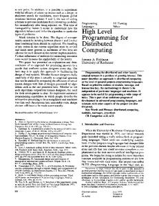
Fig. 6. (a) Transient response of the sensor to a random temperature sequence when exposed to acetone at 1/243, ammonia at 1/3 and isopropyl alcohol at 1/2187 (v/v concentration). (b) Temperature versus conductance response for acetone (one dilution step), ammonia (five steps), and ISP (seven steps).
V. EXPERIMENTAL VALIDATION We validated the active sensing model using a commercial MOX sensor (TGS2600; Figaro USA, Inc.) exposed to three different analytes (acetone, ammonia, and isopropyl alcohol). As as a proxy for an approximation, we used the heater voltage the sensor’s operating temperature. The sensor was introduced in 30 ml glass vials through a tight aperture on the cap and allowed to equilibrate with the static headspace of 10 ml of the analyte. The sensor was interfaced through a National Instruments data acquisition card (USB 6009) controlled using Matlab. Each analyte was serially diluted (1/3 dilution ratio) to determine a set of dilutions at which the sensor provided similar isothermal responses for all the analytes; this ensured that the analytes could not be discriminated without temperature modulation. To obtain the isothermal response, the sensor was exposed to each analyte for 100 seconds under a constant heater voltage of 5 V. The final dilution factors were 1/3 for ammonia (one serial dilution), 1/243 for acetone (five serial dilutions), and 1/2187 for isopropyl alcohol (seven serial dilutions). We used eight heater voltages (i.e., sensing actions) ranging from 1 to 8 V. Fig. 6(a) shows the sensor’s transient response to the three analytes for a random temperature sequence; each step was 40 s long. Information from each transient was reduced to a single observation by computing its integral response [42]. Fig. 6(b) shows the final temperature-conductivity profile, obtained by recording the sensor response to ten random voltage sequences (eight different voltage pulses per sequence) and computing the average response at each temperature. Therefore, the spread at each temperature reflects history effects. We trained a separate IOHMM for each analyte. Fig. 7(a) shows IOHMM prediction results when the sensor was exposed to acetone and driven with a random temperature sequence; prediction results for the other two targets were comparable. The IOHMMs explain a significant proportion of the variance in the response of each sensor: 90.4% for acetone, 92.1% for ammonia, and 90.1% for ISP. IOHMM predictions were shown to be less accurate at lower voltages: 1 and 2 V for acetone, 1–3 V for ammonia, and 1 V for ISP. These results are consistent with
Fig. 7. (a) Comparison between the predictions of the IOHMMs and actual sensor response to a random sequence of heater voltages in the presence of acetone. (b) Classification rate and average sequence length for a TGS2600 sensor as a function of feature acquisition costs.
the fact that the sensor response has higher variance at low temperatures; see Fig. 6(b). Moreover, IOHMM prediction errors were significantly higher for large negative temperature steps ), a reasonable result considering that cooling is pas( sive (e.g., limited by heat dispersion). Despite these estimation errors, the POMDP selects meaningful temperature sequences that predict the chemical class accurately, as we will see next. To evaluate the classification accuracy of the POMDP, we asif ; zero sumed uniform misclassification costs ( otherwise) and varied sensing costs in the range from in increments of 0.05. We ran the active-sensing algorithm five times for each analyte, resulting in 15 test cases at each cost setting. Fig. 7(b) shows the classification rate and average number of temperature steps selected by the POMDP as a function of sensing costs. Results are consistent with those obtained on the simulated sensor model: as feature acquisition costs increase, the PODMP selects fewer temperature steps at the expense of classification rate. In contrast with the simulation results in Fig. 3(b), however, these results show a more graceful degradation in classification performance as a function of the sensing costs. VI. DISCUSSION We have presented a method to optimize the temperature program of MOX sensors in real time, as the sensor reacts to its environment. The approach consists of building a dynamical model of the sensor by means of an IOHMM, and casting the resulting model into a POMDP. Our results show that IOHMMs can capture the conductance-temperature dependence and thermal dynamics of MOX sensors, and that the POMDPs
Authorized licensed use limited to: Texas A M University. Downloaded on May 14,2010 at 23:16:29 UTC from IEEE Xplore. Restrictions apply.
GOSANGI AND GUTIERREZ-OSUNA: ACTIVE TEMPERATURE PROGRAMMING FOR METAL-OXIDE CHEMORESISTORS
outperforms two “passive” classification approaches, a NN rule and a NB rule. The latter result is significant considering that the two passive classifiers were aided by a feature subset selection stage that identified the best features, whereas the POMDP operated on the entire feature space (when comparing methods, the average number of features used by each classifier was the same). The NB classifier was obtained directly from the IOHMM densities; thus, the main difference between NB and POMDP is that the latter takes state transition probabilities into consideration, which allows it to account for the sensor dynamics. This factor, combined with its adaptive feature selection capabilities, explains why the POMDP is able to consistently outperform the NB classifier (as well as the NN classifier). To this end, our results indicate that the POMDP not only selects features with high discriminatory information but also features that have low variance. As a result, the POMDP is able to exploit information both in the mean and in the variance of each class. IOHMM predictions on experimental data indicate that the model is less accurate at lower temperatures, when features are more sensitive to environmental influences. Though it is possible that the number of Gaussian components in our implemen) was insufficient to model the sensor dynamics, tation ( prediction errors could also be due to insufficient training data, since our training set consisted of only ten random temperature sequences (each temperature occurring once in a sequence), and did not contain every possible temperature transition. Similar problems with data sparsity are quite common in speech recognition, the domain where HMMs are most commonly used. A. Future Work Our work has focused on real-time prediction, but the models may also be used to generate temperature profiles offline in a more principled fashion than through trial-and-error of various waveforms (e.g., sine waves, saw tooth), and more along the line of signal exploitation methods in [4] and [10]. IOHMMs are an example of a dynamic Bayesian network with one discrete random variable (input voltage) and one continuous random variable (sensor response), but the model could be extended to incorporate additional variables. As an example, chemical concentrations could be added as a continuous random variable. The resulting Bayesian network could then model conductance-temperature and conductance-concentration relations simultaneously. At the time of this writing, we are working on extensions of the model to handle sensor drift; using a dynamic Bayesian network, drift can be modeled as a hidden variable and predicted using probabilistic inference. Interference from other gases and the effects of humidity may be incorporated in a similar fashion. In this study, we assumed uniform feature acquisition costs regardless of operating temperature, but variable sensing costs could be used to penalize higher temperatures and thus reduce power consumption. There is a great potential for deploying chemical sensors on large-scale networks [43], but such deployments are constrained due to the lack of power-aware, autonomous sensors. The active sensing approach proposed here provides a strategy for implementing energy-aware chemical sensing networks using low-cost commercial sensors.
1081
REFERENCES [1] A. P. Lee and B. J. Reedy, “Temperature modulation in semiconductor gas sensing,” Sens. Actuators, B, vol. 60, pp. 35–42, 1999. [2] A. Ortega, S. Marco, A. Perera, T. Sundic, A. Pardo, and J. Samitier, “An intelligent detector based on temperature modulation of a gas sensor with a digital signal processor,” Sens. Actuators, B, vol. 78, pp. 32–39, 2001. [3] X. Huang, F. Meng, Z. Pi, W. Xu, and J. Liu, “Gas sensing behavior of a single tin dioxide sensor under dynamic temperature modulation,” Sens. Actuators, B, vol. 99, pp. 444–450, 2004. [4] T. A. Kunt, T. J. McAvoy, R. E. Cavicchi, and S. Semancik, “Optimization of temperature programmed sensing for gas identification using micro-hotplate sensors,” Sens. Actuators, B, vol. 53, pp. 24–43, 1998. [5] A. Vergara, E. Llobet, J. Brezmes, P. Ivanov, X. Vilanova, I. Gracia, C. Cane, and X. Correig, “Optimised temperature modulation of metal oxide micro-hotplate gas sensors through multilevel pseudo random sequences,” Sens. Actuators, B, vol. 111–112, pp. 271–280, 2005. [6] Y. Bengio and P. Frasconi, “An input output HMM architecture,” Advances in Neural Information Processing Systems, pp. 427–434, 1995. [7] L. Rabiner and B. Juang, “An introduction to hidden Markov models,” IEEE ASSP Mag., vol. 3, pp. 4–16, 1986. [8] L. P. Kaelbling, M. L. Littman, and A. R. Cassandra, “Planning and acting in partially observable stochastic domains,” Arti. Intell., vol. 101, pp. 99–134, 1998. [9] R. Gosangi and R. Gutierrez-Osuna, “Active chemical sensing with partially observable Markov decision processes,” in Proc. 13th Int. Symp. Olfaction and Electronic Nose, Brescia, Italy, 2009. [10] A. Vergara, E. Llobet, J. Brezmes, X. Vilanova, P. Ivanov, I. Gracia, C. Cane, and X. Correig, “Optimized temperature modulation of microhotplate gas sensors through pseudorandom binary sequences,” IEEE Sensors J., vol. 5, pp. 1369–1378, 2005. [11] R. Bajcsy, “Active perception,” Proc. IEEE, vol. 76, pp. 966–1005, 1988. [12] J. Aloimonos, I. Weiss, and A. Bandyopadhyay, “Active vision,” Int. J. Comput. Vision, vol. 1, pp. 333–356, 1988. [13] D. H. Ballard, “Animate vision,” Artif. Intell., vol. 48, pp. 57–86, 1991. [14] J. J. Gibson, The Ecological Approach to Visual Perception. Boston, MA: Houghton Mifflin, 1979. [15] L. Paletta and A. Pinz, “Active object recognition by view integration and reinforcement learning,” Robot. Autonomous Syst., vol. 31, pp. 71–86, 2000. [16] J. Denzler and C. M. Brown, “Information theoretic sensor data selection for active object recognition and state estimation,” IEEE Trans. Pattern Anal. Mach. Intell., vol. 24, pp. 145–157, 2002. [17] M. A. Sipe and D. Casasent, “Feature space trajectory methods for active computer vision,” IEEE Trans. Pattern Anal. Mach. Intell., vol. 24, pp. 1634–1643, 2002. [18] L. Mihaylova, T. Lefebvre, H. Bruyninckx, K. Gadeyne, and J. D. Schutter, “Active sensing for robotics-A survey,” in Proc. 5th Int. Conf. Numerical Methods and Appl., 2002, pp. 316–324. [19] H. Zhou and S. Sakane, “Mobile robot localization using active sensing based on Bayesian network inference,” Robot. Autonomous Syst., vol. 55, pp. 292–305, 2007. [20] D. Fox, W. Burgard, and S. Thrun, “Active markov localization for mobile robots,” Robot. Autonomous Syst., vol. 25, pp. 195–207, 1998. [21] G. C. H. E. de Croon, I. G. Sprinkhuizen-Kuyper, and E. O. Postma, “Comparing active vision models,” Image Vision Comput., vol. 27, pp. 374–384, 2009. [22] T. Arbel and F. P. Ferrie, “Entropy-based gaze planning,” Image and Vision Comput., vol. 19, pp. 779–786, 2001. [23] T. Nakamoto, N. Okazaki, and H. Matsushita, “Improvement of optimization algorithm in active gas/odor sensing system,” Sens. Actuators, A, vol. 50, pp. 191–196, 1995. [24] C. E. Priebe, D. J. Marchette, and D. M. Healy, “Integrated sensing and processing decision trees,” IEEE Trans. Pattern Anal. Mach. Intell., vol. 26, pp. 699–708, 2004. [25] D. Waagen, H. A. Schmitt, and N. Shah, “Activities in integrated sensing and processing,” in Proc. Intell. Sensors, Sensor Networks and Information Process. Conf., 2004, pp. 295–300. [26] C. Kreucher, K. Kastella, and A. O. Hero, “Sensor management using an active sensing approach,” Signal Process., vol. 85, pp. 607–624, 2005. [27] R. Gutierrez-Osuna, “Pattern analysis for machine olfaction: A review,” IEEE Sensors J., vol. 2, pp. 189–202, 2002. [28] S. Ji and L. Carin, “Cost-sensitive feature acquisition and classification,” Pattern Recognit., vol. 40, pp. 1474–1485, 2007.
Authorized licensed use limited to: Texas A M University. Downloaded on May 14,2010 at 23:16:29 UTC from IEEE Xplore. Restrictions apply.
1082
IEEE SENSORS JOURNAL, VOL. 10, NO. 6, JUNE 2010
[29] A. V. Nefian, L. Liang, X. Pi, X. Liu, and K. Murphy, “Dynamic Bayesian networks for audio-visual speech recognition,” EURASIP J. Appl. Signal Process., pp. 1274–1288, Jan. 2002, DOI=10.1155/ S1110865702206083 http://dx.doi.org/10.1155/S1110865702206083, http://portal.acm.org/beta/citation.cfm?id=1283223. [30] C. H. Papadimitriou and J. N. Tsitsiklis, “The complexity of Markov decision processes,” Math. Oper. Res., vol. 12, pp. 441–450, 1987. [31] S. Zhang, C. Xie, H. Li, Z. Bai, X. Xia, and D. Zeng, “A reaction model of metal oxide gas sensors and a recognition method by pattern matching,” Sens. Actuators, B, vol. 135, pp. 552–559, 2009. [32] P. K. Clifford and D. T. Tuma, “Characteristics of semiconductor gas sensors II. Transient response to temperature change,” Sens. Actuators, vol. 3, pp. 255–281, 1982. [33] R. Ionescu, E. Llobet, S. Al-Khalifa, J. W. Gardner, X. Vilanova, J. Brezmes, and X. Correig, “Response model for thermally modulated tin oxide-based microhotplate gas sensors,” Sens. Actuators, B, vol. 95, pp. 203–211, 2003. [34] S. Nakata, K. Takemura, and K. Neya, “Non-linear dynamic responses of a semiconductor gas sensor: Evaluation of kinetic parameters and competition effect on the sensor response,” Sens. Actuators, B, vol. 76, pp. 436–441, 2001. [35] J. Ding, T. J. McAvoy, R. E. Cavicchi, and S. Semancik, “Surface state trapping models for SnO2-based microhotplate sensors,” Sens. Actuators, B, vol. 77, pp. 597–613, 2001. [36] S. Wlodek, K. Colbow, and F. Consadori, “Signal-shape analysis of a thermally cycled tin-oxide gas sensor,” Sens. Actuators, B, vol. 3, pp. 63–68, 1991. [37] E. Llobet, X. Vilanova, J. Brezmes, D. Lopez, and X. Correig, “Electrical equivalent models of semiconductor gas sensors using PSpice,” Sens. Actuators, B, vol. 77, pp. 275–280, 2001. [38] K. Fukunaga, Introduction to Statistical Pattern Recognition, 2nd ed. Reading, MA: Academic Press, 1990. [39] T. M. Mitchell, Machine Learning, 1 ed. New York: McGraw-Hill, 1997. [40] J. Kittler, “Feature set search algorithms,” Pattern Recognition and Signal Processing, pp. 41–60, 1978.
[41] G. John, R. Kohavi, and K. Pfleger, “Irrelevant features and the subset selection problem,” in Proc. Int. Conf. Mach. Learning, 1994, pp. 121–129. [42] A. Hierlemann and R. Gutierrez-Osuna, “Higher-order chemical sensing,” Chem. Rev., vol. 108, pp. 563–613, 2008. [43] D. Diamond, S. Coyle, S. Scarmagnani, and J. Hayes, “Wireless sensor networks and chemo-/biosensing,” Chem. Rev., vol. 108, pp. 652–679, 2008.
Rakesh Gosangi received the B.Tech. degree in computer science and engineering from the Indian Institute of Technology Madras (IITM), Chennai, India, in 2007. He is currently working towards the Ph.D. degree at Texas A&M University, College Station. His research interests include pattern recognition, probabilistic graphical models, chemical sensors, and machine olfaction.
Ricardo Gutierrez-Osuna (M’00) received the B.S. degree in electrical engineering from the Polytechnic University of Madrid, Madrid, Spain, in 1992, and the M.S. and Ph.D. degrees in computer engineering from North Carolina State University, Raleigh, in 1995 and 1998, respectively. From 1998 to 2002, he served on the faculty at Wright State University. He is currently an Associate Professor of Computer Engineering at Texas A&M University. His research interests include pattern recognition, neuromorphic computation, chemical sensor arrays, and audio-visual speech processing.
Authorized licensed use limited to: Texas A M University. Downloaded on May 14,2010 at 23:16:29 UTC from IEEE Xplore. Restrictions apply.