Activity Recognition using Dynamic Subspace Angles

Activity Recognition using Dynamic Subspace Angles Binlong Li, Mustafa Ayazoglu, Teresa Mao, Octavia I. Camps and Mario Sznaier ∗ Dept. of Electrical and Computer Engineering, Northeastern University, Boston, MA 02115 http://robustsystems.ece.neu.edu

Abstract

ity reduction methods (e.g. PCA or manifold embeddings). Volumetric approaches process the video data as a volume of pixels and use local features that are 3D generalizations of standard image features such as corners and spatial-temporal filter responses. Indeed, a significant portion of the most recent work in activity recognition has been inspired by the success of using local features for object recognition [5, 11, 12, 9]. However, both, non-parametric and volumetric approaches are limited by the inherent local nature of the features used and the lack of strong relations among features across frames. In contrast, parametric timeseries approaches use dynamical models of the motions to exploit temporal relations across frames. Thus, they are better equipped to model and recognize complex activities that last longer. Examples of parametric approaches include hidden Markov models (HMMs) and linear dynamical systems which can be thought of as a generalization of HMMs, where the state vector can take continuous values in Rd and where d is the dimensionality of the state space. However, a drawback of these methods is that they must assume a dynamical model, which is often too simplistic, and that they must estimate the model parameters from extensive experimental data, often corrupted by noise.

Cameras are ubiquitous everywhere and hold the promise of significantly changing the way we live and interact with our environment. Human activity recognition is central to understanding dynamic scenes for applications ranging from security surveillance, to assisted living for the elderly, to video gaming without controllers. Most current approaches to solve this problem are based in the use of local temporal-spatial features that limit their ability to recognize long and complex actions. In this paper, we propose a new approach to exploit the temporal information encoded in the data. The main idea is to model activities as the output of unknown dynamic systems evolving from unknown initial conditions. Under this framework, we show that activity videos can be compared by computing the principal angles between subspaces representing activity types which are found by a simple SVD of the experimental data. The proposed approach outperforms state-of-the-art methods classifying activities in the KTH dataset as well as in much more complex scenarios involving interacting actors.

1. Introduction

In this paper we propose a time-series approach for activity recognition that, in contrast with previous approaches, requires neither assuming nor identifying a dynamical model. Instead, we simply hypothesize that the temporal data is the output trajectory of an underlying, unknown linear (possibly slowly varying) dynamical system. In this context, different realizations of the same activity correspond to trajectories of the same system in response to different initial conditions. Exploiting the fact, derived from realization theory, that these trajectories are constrained to evolve in the same subspace (directly determined from the experimental data) allows for measuring the similarity between activities by simply computing the angle between the associated subspaces. While the approach outlined above works well for low levels of noise, its performance degrades substantially as the noise level increases. To improve robustness against noise, rather than directly clustering activities based on the angle of the corresponding subspaces, we

Activity recognition from video is central to many applications, including visual surveillance, assisted living for the elderly, and human computer interfaces. In recent years, a large number of researchers have addressed this problem as evidenced by several extended survey papers on this topic [1, 4, 10, 18]. Current approaches to modeling and recognizing actions of single actors can be classified into one of three major classes: nonparametric, volumetric, and parametric timeseries approaches [18]. Nonparametric methods rely on features extracted at the frame level that are then matched against stored templates. The templates can be 2D (e.g. motion history images), 3D (e.g. generalized cylinders in the joint space-time (x, y, t) domain), or use dimensional∗ This work was supported in part by NSF grants IIS–0713003 and ECCS–0901433, AFOSR grant FA9550–09–1–0253, and the Alert DHS Center of Excellence under Award Number 2008-ST-061-ED0001.

3193

first apply a discriminative canonical correlation [8] transformation to simultaneously decrease the inter-class and increase the intra-class distances. Finally, the resulting subspaces are used to train a support vector machine (SVM) to classify the activities. The main result of the paper shows that the proposed approach outperforms existing ones when tested using a standard database (KTH) containing video clips of different single actor activities. Further, our approach can also handle, without modifications, the much more difficult case where the scenes contain multiple actors and activities are characterized by the interaction between agents, rather than individual activities. The paper is organized as follows. Section 2 gives a brief summary of background material on dynamical systems and canonical correlations between subspaces. Section 3 gives the details of the proposed approach and section 4 discusses experimental results comparing the proposed approach against previously reported results on activity recognition. Finally, section 5 gives final remarks and discusses future directions.

It should be noted that an important limitation to the practical use in computer vision of models of the form (1), is that one must assume or estimate the dimensions and values of the matrices A and C and the initial vector xo . Further, given a finite number of measurements of yk , the set of triples (A, C, xo ) that could have generated this data is not unique1 . Finally, attempting to jointly identify the dynamics (A, C) and the initial condition xo leads to computationally challenging non convex problems. To avoid these difficulties, in this paper we will not work directly with the model representation (1). Instead, motivated by subspace identification methods [13], we will work with the block Hankel matrices of its output sequences as defined next. Given a sequence of output measurements from the system (1), yo , y1 , . . . , its associated (block) Hankel matrix Hy is:   yo y1 y2 ... ym  y1 y2 y3 . . . ym+1     y2 y y . . . ym+2  3 4   Hy =   (2) .. .. .. .. ..   . . . . .    ym−1 ym ym+1 . . . y2m−1  ym ym+1 ym+2 . . . y2m

2. Background 2.1. Dynamical Systems and the Hankel Matrix

As we show in section 3, the special structure of this matrix encapsulates the dynamic information of the system.

Dynamical systems are a powerful tool to work with temporally ordered data. They have been used in several applications in computer vision, including tracking, human recognition from gait, activity recognition, and dynamic texture. The main idea, is to use a dynamical system to model the temporal evolution of a measurement vector yk ∈ Rn as a function of a relatively low dimensional state vector xk ∈ Rd that changes over time. For example, depending on the application, the measurement vector yk can represent the coordinates of a tracked target at time k, or the pixel values of an image captured at time k. Then, the dynamical model can be used both, as a generative model, for example to predict the location of the target in the next frame or to generate a new video sequence of dynamic texture, or as a nominal model, for example to characterize activities or dynamic textures for recognition or classification. The simplest dynamical model is a linear time invariant (LTI) system of the form: yk xk

= =

Cxk Axk−1 + wk ,

xo given

2.2. Canonical Correlations of Linear Subspaces Recognition and classification problems can often be posed as a vector classification task, where an unknown vector (for example, a rasterized image) has to be assigned to one of a set of training classes represented as a linear subspace learned from a set of labeled vectors (images). The separation between classes can be measured using canonical correlations, also known as principal or canonical angles, which are defined as follows: Given two subspaces F and G such that p = dim(F ) ≥ dim(G) = q ≥ 1, the cosine of the smallest principal angle θ1 (F, G) = θ1 ∈ [0, π/2] between F and G is defined by cos θ1 = max max uT v kuk2 = kvk2 = 1 u∈F v∈G

Assuming that the maximum is obtained at u = u1 , v = v1 , then θ2 (F, G) is defined as the smallest angle between the orthogonal complement of F with respect to u1 and that of G with respect to v1 , and so forth, until one of the subspaces is empty. Then, the canonical correlations are defined as:

(1)

where both the state and the measurement equations are linear, the matrices A and C are constant over time, and where wk ∼ N (0, Q) is uncorrelated zero mean Gaussian measurement noise. The dimension of the state vector, d, is the order (memory) of the system and is a measure of its complexity.

cos θk = max max uT v = uTk vk kuk2 = kvk2 = 1 u∈F v∈G

1 This

is related to the concepts of consistency set and diameter of information [16], Chapter 10.

3194

subject to the constraints

by first transforming the data using the method proposed in [8] followed by a support vector machine (SVM) that selects the best matching subspace. The full details of the classification algorithm are given in section 3.2.

uTj u = 0 , vjT v = 0 , j = 1, 2, . . . , k − 1 When the subspaces are defined as the range of two matrices A and B, the canonical correlations can be computed by performing a singular value decomposition (SVD) as follows [2]. Let PA and PB be unitary bases for the subspaces spanned by A and B and let M = PAT PB . Then, the canonical correlations between A and B are given by the singular values of M . Intuitively, the canonical correlations measure the angles between the closest vectors from the two subspaces. A high canonical correlation value corresponds to a small subspace angle and to subspaces that are close to each other. On the other hand, a small canonical correlation corresponds to a subspace angle near π/2 or subspaces that are close to orthogonal. Thus, in classification applications, classes that have higher canonical correlations are more separated and easier to discriminate. Indeed, given a set of training classes represented by subspaces, it is possible to improve the classification performance and robustness to noise by using discriminant canonical correlations (DCC) [8]. This is accomplished by first applying a linear transformation to the given data in a way to maximize the canonical correlations of with-in classes while minimizing the canonical correlations of between-classes.

3.1. Dynamic Subspaces Angles (DSA) In this section we present the key observation that motivates this paper: in the absence of noise, all the output trajectories of the dynamical system (1) lie on a single subspace that can be determined from the experimental data from a single realization. Theorem: The principal angles between the subspaces spanning the columns of the Hankel matrices corresponding to trajectories of the same dynamical system in response to potentially different initial conditions are zero. Proof: Let Hy be a block Hankel matrix of an output trajectory of the dynamical system (1) when wk ≡ 0. Then, using (1) we have yk = Cxk = CAxk−1 = CA2 xk−2 = · · · = CAk xo Thus, the Hankel matrix Hy can be rewritten as: 

yo y1 y2 .. .

    Hy =     ym−1 ym

3. Proposed Approach

y1 y2 y3 .. .

y2 y3 y4 .. .

... ... ... .. .

ym ym+1 ym+2 .. .

ym ym+1

ym+1 ym+2

... ...

y2m−1 y2m

      = ΓX    (3)

We propose to model activities as the responses of unknown LTI systems with unknown initial conditions. In this scenario, two realizations of the same activity are explained by a single dynamical system with different initial conditions, while different activities are explained by different dynamical systems. Then, the problem of activity recognition reduces to: Comparison of Output Trajectories Problem: Given two temporal sequences, decide whether or not they can be explained as two output trajectories of the same dynamical system, possibly with different initial conditions. In the sequel, we show that the answer to this question can be found in the Hankel matrices of the output sequences under consideration. In particular, we show that in the noise-less case, all the output trajectories of a system, regardless of the initial condition, lie in a single subspace that can be used to represent the corresponding activity and that is easily determined from the Hankel matrix of the experimental data from a single realization. Based on this result, we propose to classify unknown activities by using canonical correlations to compare their associated subspaces to those obtained from training labeled data. To further improve robustness to noise and variations due to different actors performing the activities, classification is actually done

where 

C CA .. .



    Γ=  and   m CA

 X = xo

x1

...

xm



and X is a matrix containing the state trajectories as its columns. From (3) it follows that regardless of the initial condition, the columns of Hy and Γ span the same subspace. Hence, the principal angles between subspaces spanned from the columns of the Hankel matrices of output trajectories from the same system must be zero. q.e.d. The significance of this result, as explained next, is that output trajectories can be compared in terms of dynamic subspaces angles (DSA), defined as the canonical correlations between the subspaces spanned by their Hankel matrices. Note that in realistic situations, wk 6≡ 0. In this case, the angle between subspaces for two realizations of the same activity will not be zero. However, since this angle is a continuous function of the entries of Hy , angles corresponding to (noisy) trajectories of the same system will still be small, 3195

when compared against the subspace angles of different systems. To illustrate this effect, consider a simple onedimensional version of (1) with C = 1, A = 1 and initial condition x0 = 1. Thus, yk = xk = 1 for all k. Assume now that, due to noise, the first three measurements of y yield yo = 0.95, y1 = 0.975 and y2 = 1.012. It can be easily shown that the minimal order of a system required to generate these measurements is two. Indeed, simple algebra shows that the sequence yk could have been generated by the triple       2.5 1 0.95 C= 1 0 , A= , x0 = −1.5 0 −1.4 Hence, a moderate amount of noise (less than 5%) can lead to substantial error in estimating the dynamics and initial condition. On the other hand, the column subspaces of the nominal and noisy Hankel matrices are given by:     −0.71 −0.71 −0.70 −0.72 Unom = , Unoisy = , −0.71 0.71 −0.72 0.70 (4) with the angle between the first vector of each subspace ∼ 0.014. Thus, using subspace angles instead of identifying and comparing dynamical models provides substantial robustness against errors in estimating y. Applying a canonical correlation maximizing transformation [8] to the subspaces prior to computing the angles results in an even larger separation, allowing for successfully classifying activities from realistic video sequences, where y is affected by noise, and correspondence errors.

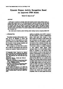
Figure 1. Overview of Activity Recognition Using Dynamic Subspace Angles

2. Hankel Matrices Assembly Next, the measurements for each video are collected in a Hankel matrix representing its temporal informa(k) tion. Let Hi ∈ Rmn×(Fki −mn) denote the Hankel matrix for video i of class k, i = 1, . . . , Nk , and k = 1, . . . , c where m is the number of row blocks and Fki is the number of frames in the video. Thus, there are a total of N Hankel matrices: (1) (1) (c) (c) {{H1 , . . . , HN1 }, . . . , {H1 , . . . , HNc }}. 3. DCC

3.2. Activity Recognition Using DSA

The discriminant function for canonical correlations among the subspaces spanned by the columns of the Hankel matrices (1) (1) (c) (c) {{H1 , . . . , HN1 }, . . . , {H1 , . . . , HNc }} is computed using the algorithm in [8] (repeated here for completeness):

In this section we describe the details for training and testing a system to recognize activities using DSA, given a labeled database consisting of c classes of actions, with Nk sample P videos for class k, with k = 1, . . . , c and N = k Nk . Figure 1 shows a diagram illustrating all the required steps.

(a) Find an orthogonal column basis for each Han(k)

(k) T

(k)

(k)

(k) T

kel matrix: Let Hi Hi ≈ Pi Λ i P i (k) (k) mn×d where Pi ∈ R and Λi are the eigenvalue and eigenvector matrices of the d largest eigenvalues, respectively. (b) Find an orthogonal transformation matrix T ∈ Rmn×q with q ≤ mn: i. T ← Imn ii. Do iterate the following: iii. For all i do QR-decomposition: T T Pi = Φi ∆i → Pi0 = Pi ∆i −1 iv. For every pair i, j do SVD Pi0T T T T Pj0 = Qij ΛQTij

Training Procedure 1. Feature Extraction and Tracking The first step is to collect temporal features from all the videos in the training database. The proposed method can be used with different type of features, the only requirement is that they are temporally ordered. They can be, for example, a set of point features and/or dimensions of bounding boxes tracked across frames, or HOGs values in a set of bins across time. In the se(i) quel we will use yj ∈ Rn to denote the feature vector extracted from video i at frame j. 3196

PN P 0 v. Compute Sb = i=1 l∈Bi (Pl Qli 0 0 0 T Pi Qil )(Pl Qli − Pi Qil ) , where Bi {j|Hj ∈ / Ci } PN P 0 vi. Compute Sw = i=1 l∈Wi (Pk Qki Pi0 Qik )(Pk0 Qki − Pi0 Qki )T , where Wi {j|Hj ∈ Ci } vii. Compute mn eigenvectors −1 {ti }mn S S , T ← [t b 1 , . . . , tnm ] i=1 w viii. End ix. T ← [t1 , . . . , tq ]

− = − = of

Figure 2. Feature Extraction: Three frames from the KTH database for hand waving and walking and their responses to a Gabor 3D spatial-temporal filter. The two strongest clusters are tracked over time (red and green trajectories).

(c) Apply T to the left orthogonal matrix of every 0(k) (k) Hankel matrix: Pi = T T Pi 4. SVM Training Train a multi-class support vector machine using the 0(k) first r columns of Pi , i = 1, . . . , Nk , as sample feature vectors for class k, k = 1, . . . , c. Testing Procedure are:

4.1.1

Feature Extraction

A variety of possible features can be used to capture the dynamics of the activities. For these experiments we chose to use the two strongest connected components of the response to a Gabor 3D spatial-temporal filter proposed in [5] and the width of the bounding box (measured with respect to the centroid of the person performing the activity), tracked across the duration of the video. The response function has the form R = (I ∗ g ∗ hev )2 + (I ∗ g ∗ hod )2 where g is a 2D Gaussian spatial smoothing kernel and hev = 2 2 2 2 − cos(2πtω)e−t /τ and hod = − sin(2πtω)e−t /τ are a quadratic pair of 1D Gabor filters. In our experiments we used σ = 0.8 and τ = 1.2. Features were tracked using a LK tracker. Figure 2 shows sample frames for two activities, their filter response and the tracks for the two strongest clusters.

The steps to classify a video sequence

1. Collect features. 2. Assemble the Hankel matrix of the measurements, Hy . 3. Compute the svd of Hy HyT = P DP T . 4. Apply the DCC Transformation T to P : P 0 = T T P . 5. Use the trained SVM to assign a label based on the first r columns of P 0 .

4. Experiments

Finally, the feature vector y ∈ R6 for each frame consists of the following six numbers: the two coordinates for each of the two strongest clusters, the distance between the left side of the bounding box and the person’s centroid, and the distance between the person’s centroid and the right side of the bounding box2 .

4.1. KTH Database The proposed approach was tested using six types of human activities (walking, running, boxing, hand waving, hand clapping, and jogging) from the widely used KTH activity dataset [17]. The activities were performed by 25 subjects in four scenarios: outdoors, outdoors with scale variation, outdoors with different clothing, and indoors. All sequences have an homogeneous background and were captured by a stationary camera. Unfortunately, comparing performance results against results published in the literature is difficult, since different authors use different experimental protocols [6]. We chose to follow the most commonly used experimental protocol which was described in the original paper [17]. This protocol partitions the data into a training set (subjects: 1,4,11,12,13,14,15,16), a validating set (subjects: 17,18,19,20,21,23,24 25) to tune system parameters, and a testing set (subjects: 2,3,5,6,7,8,9,10,22) to evaluate performance.

4.1.2

Hankel Matrix Assembly

The Hankel matrices were assembled using the features from all the frames. The dimensions were chosen such that the Hankel matrices are as square as possible. Since the average number of frames per video in the database is 200 and the dimension of the feature vector n = 6, we chose m = 24 and hence, the Hankel matrices have mn = 144 rows and a variable number of columns. 3197

using the validation set. The best performance was obtained for r = 1 (See Figure 4). 4.1.5

Tests and Performance Evaluation

We conducted three tests with the KTH dataset. The first one, tested the trained system using the testing set as indicated by the experimental protocol in [17]. The second test was to evaluate the benefit of using DCC to increase performance. Finally, the third test was designed to test whether using the structure and information encoded in the Hankel matrices provided any added value over using DCC on a set of vectors formed by the tracked features in sub-sequences of the videos. Figure 3. Singular values of the Hankel matrices for all the videos in the training and validating sets.

Performance Evaluation The overall accuracy rate of the proposed approach is 93.6%. Tables 1 and 2 show that this performance is better than previously reported performances using the same experimental protocol. The interclass confusion matrix using the test set is given in Table 3. Table 1. Comparison of overall performance for KTH dataset using experimental protocol defined in [17]

Algorithm Ours Wang et al. [19] Laptev et al. [9] Niebles et al. [12] Wong et al. [20] Schuldt et al. [17] Figure 4. Classification performance for the training and validation sets as the number of basis vectors r used to train the SVM are varied. The best performance was obtained for r = 1.

4.1.3

Benefits of Using DCC We measured the performance of the system when skipping the DCC step (in effect, setting the transformation T as the identity). It was observed that the overall performance drops to 89.35% if DCC is not used.

DCC

The number of vectors for the Hankel matrix bases, d, was set to 21. Figure 3 shows a plot of the singular values for the Hankel matrices for the videos in the training and validating sets. The figure shows that the singular values decay quickly and that the energy for beyond the 21th singular value is negligible. 4.1.4

P erf. 93.6 92.1 91.8 91.3 86.7 71.5

Benefits of Using Hankel Matrices Kim et al. [8] proposed to use DCC for object and object category recognition where the data consist of rasterized images, captured under different settings such as different illuminations and viewpoints. One could try to use the same approach to perform activity recognition by applying it to the frames in the activity videos. In this case, the classes are the activities, and each frame is considered as a sample of an activity. However, this approach would not fully exploit the temporal information since DCC is invariant to the ordering of the data. Thus, a better way of using DCC with temporal data would be to cut each video into small sub-sequences, rasterize each sub-sequence into a vector, and apply DCC to these vectors. In this way, each sample would capture a snippet of temporal information. Note that from an implementation point of view, the difference between this approach and the

SVM Training

We use a non-linear support vector machine with 2nd degree inhomogeneous poly-kernel using a one-against-rest approach from the SVM toolbox [3]. The number of vectors r from the transformed bases was chosen by varying it from 1 to 32 and evaluating the classification performance 2 All measurements are normalized with respect to the height of the bounding box to make them invariant to different people’s height.

3198

Table 2. Comparison of overall performance for KTH dataset using experimental protocol defined in [17] as reported in [19]

Harris3D Cuboids Hessian Dense

HOG3D 89 90 84.6 85.3

HOG/HOF 91.8 88.7 88.7 86.1

HOG 80.9 82.3 77.7 79

HOF 92.1 88.2 88.6 88

Cuboids 89.1 -

ESU RF 81.4 -

Hankel 93.06 -

Table 3. Inter-class confusion matrix for KTH (testing sets) using the proposed approach.

Boxing HClapping HWaving Walking Running Jogging

Boxing 97.22 2.78 0 0 0 0

HClapping 0 94.44 13.89 0 0 0

HWaving 0 0 86.11 0 2.78 0

Walking 0 0 0 97.22 0 0

Running 2.78 0 0 0 83.33 0

Jogging 0 2.78 0 2.78 13.89 100

to large computational requirements and manual alignment of the videos.

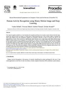
4.2. TV Interaction Database The proposed approach was also tested with the more challenging TV Interaction dataset [14] to classify two types of human interactions (hand shaking and high-five). The database has 50 videos of each type that are short clips from TV sitcoms. Figure 6 (a) shows sample frames illustrating the level of clutter and scene complexity in this database.

Figure 5. Advantage of using Hankel matrices over using DCC with sub-sequences to recognize KTH activities.

proposed one in this paper is minimal: when we use Hankel matrices, each sample vector corresponds to a sub-sequence (a column of the Hankel matrix) that completely overlaps other sample sub-sequences (the previous and next columns of the Hankel matrix), except for two frames3 . However, it should be emphasized that the effect of this seemingly minor difference is quite significant as shown in Figure 5, where the performance of the two approaches in classifying the KTH test set as the number of basis vectors d is varied are compared. There, the best performance using DCC alone is 81.48 % while using Hankel matrices together with DCC achieves a performance of 93.6%. It should be noted, that Kim and Cipollal [7] proposed a different generalization to DCC for handling temporal data through tensors. However, using their method to recognize activities requires significant down-sampling of the data due

(a)

(b) Figure 6. (a) Sample frames from the TV Interaction Database [14]. (b) HOG features.

4.2.1

Feature Extraction

Due to the level of clutter and ego-motion in the videos, we chose to use as features the histogram of gradients (HOG)

3 In our experiments, this corresponds to an overlap of 22 frames out of a 24 frames sub-sequence.

3199

and track the temporal evolution of the angles of the gradients. We computed HOG for each actor (using the bounding boxes provided in the dataset) using a 16 × 8 grid. as shown in Figure 6 (b). Then, the feature vector for frame k is a vector y ∈ R256 made up of the 128 HOG angles for each actor. 4.2.2

[3] S. Canu, Y. Grandvalet, V. Guigue, and A. Rakotomamonjy. Svm and kernel methods matlab toolbox, 2005. 6 [4] C. Cedras and M. Shah. Motion-based recognition: A survey. Image and Vision Computing, 13(2):129–155, 1999. 1 [5] P. Dollar, V. Rabaud, G. Cotteell, and S. Belongie. Behavior recognition via sparse spatio-temporal features. In VS-PETS, pages 65–72, 2005. 1, 5 [6] Z. Gao, M. Chen, A. G. Hauptmann, and A. Cai. Comparing evaluation protocols on the kth dataset. In Human Behavior Understanding, ICPR, pages 88–100. Springer, 2010. 5 [7] T. Kim and R. Cipolla. Canonical correlation analysis of video volume tensors for action categorization and detection. IEEE Trans. on Pattern Analysis and Machine Intelligence, 31(8):1415–1428, Aug. 2009. 7 [8] T. Kim, J. Kittler, and R. Cipolla. Discriminative learning and recognition of image set classes using canonical correlations. IEEE Trans. on Pattern Analysis and Machine Intelligence, 29(6):1005–1018, Jun 2007. 2, 3, 4, 6 [9] I. Laptev, M. Marszalek, C. Schmid, and B. Rozenfeld. Learning realistic human actions from movies. Computer Vision and Pattern Recognition, 2008. CVPR 2008. IEEE Conference on DOI - 10.1109/CVPR.2008.4587756, pages 1–8, 2008. 1, 6 [10] T. B. Moeslund, A. Hilton, and V. Kr¨uger. A survey of advances in vision-based human motion capture and analysis. Computer Vision and Image Understanding, 104(2):90–126, 2006. 1 [11] J. Niebles, H. Wang, and L. Fei-Fei. Unsupervised learning of human action categories using spatial-temporal words. International journal of computer vision, 79(3):299–318, 2008. 1 [12] J. C. Niebles, C.-W. Chen, and L. Fei-Fei. Modeling temporal structure of decomposable motion segments for activity classification. ECCV, pages 1–14, Jul 2010. 1, 6 [13] P. V. Overschee and B. D. Moor. N4SID: subspace algorithms for identification of combined deterministic– stochastic systems. Automatica, 30(1):75–93, 1994. 2 [14] A. Patron-Perez. Tv human interaction dataset. 7 [15] A. Patron-Perez, M. Marszalek, A. Zisserman, and I. Reid. High five: Recognising human interactions in tv shows. In British Machine Vision Conference, 2010. 8 [16] R. S´anchez Pe˜na and M. Sznaier. Robust Systems Theory and Applications. Wiley & Sons, Inc., 1998. 2 [17] C. Sch¨uldt, I. Laptev, and B. Caputo. Recognizing human actions: A local svm approach. In ICPR, 2004. 5, 6, 7 [18] P. Turaga, R. Chellappa, V. S. Subrahmanian, and O. Udrea. Machine recognition of human activities: A survey. IEEE Trans. on Circuits and Systems for Video Technology, 18(11):1473–1488, Nov 2008. 1 [19] H. Wang, M. Ullah, A. Klaser, I. Laptev, and C. Schmid. Evaluation of local spatiotemporal features for action recognition. In British Machine Vision Conference, pages 1–11, 2009. 6, 7 [20] S. Wong, T. Kim, and R. Cipolla. Learning motion categories using both semantic and structural information. 2007 IEEE Conference on Computer Vision and Pattern Recognition, pages 1–6, 2007. 6

Hankel Matrix Assembly, DCC, and SVM Steps

The Hankel matrices were assembled using the HOG features using m = 4. Hence, they have mn = 1024 rows and a variable number of columns depending on the number of frames in the clip. For the estimation of T during the DCC step, we used d = 6 and we kept one vector (r = 1) for the SVM training. 4.2.3

Performance Evaluation

We tested the classification performance following the experimental protocol used by the creators of the database [15] achieving a overall performance of 68% which is significantly higher compared to the performance of 54.45% reported in [15].

5. Conclusion We proposed a new time-series approach for human activity recognition that does not need to identify a model. Instead, it exploits the dynamic information encoded in the structure of Hankel matrices built from the data. We showed that trajectories corresponding to the same activity live in a subspace and that the DSA – i.e. the canonical correlations between the associated subspaces – can be used to classify the activities. Our experiments show that both, using DCC to increase the separation between classes, and using Hankel matrices to capture the temporal information, result in significant improvements of the overall classification performance. The proposed approach was tested with the KTH database and the much more challenging TV Interaction database, achieving an overall performance of 93.6% and 68%, respectively, which are significantly higher than the highest reported performance using the same experimental protocols. In the future, we plan to explore the effect of using different types of features, more complex activities and the possibility of using the dynamic subspaces as generative models.

References [1] J. K. Aggarwal and Q. Cai. Human motion analysis: A review. Computer Vision and Image Understanding, 73(3):428–440, 1999. 1 [2] A. Bjorck and G. Golub. Numerical methods for computing angles between linear subspaces. Mathematics and Computation, 27(123):579–594, July 1973. 3

3200