ory,â in PhD Thesis, Merton College, Universoty of OXford,. 1998. [15] M. Isard and A. Blake, âContour tracking by stochastic propagation of conditional density,â ...
Activity Recognition Using the Dynamics of the Configuration of Interacting Objects Namrata Vaswani, Amit Roy Chowdhury, Rama Chellappa
Abstract:
arately and then learning their interactions, we propose a different approach to the problem using Kendall’s statistical shape theory [3]. We model an activity by the polygonal ‘shape’ formed by joining the locations of these point objects (henceforth referred to as ‘points’) at any time and its deformation over time. This provides a compact global framework to model the motion of interacting moving objects over time. We are able to identify “spatial” abnormalities, e.g. deviations from the normal path, as well as “temporal” abnormalities, e.g. sudden stopping for prolonged periods of time when the normal activity should be continuous motion.
Monitoring activities using video data is an important surveillance problem. A special scenario is to learn the pattern of normal activities and detect abnormal events from a very low resolution video where the moving objects are small enough to be modeled as point objects in a 2D plane. Instead of tracking each point separately, we propose to model an activity by the polygonal ‘shape’ formed by joining the locations of these point masses at any time , and its deformation over time. We learn the mean shape and the dynamics of the shape change using hand-picked location data (no observation noise) and define an abnormality detection metric for the simple case of a test sequence with negligible observation noise. For the more practical case where observation (point locations) noise is large and cannot be ignored, we use a particle filter to estimate a probability density function (pdf) for the actual shape given the noisy observations upto the current time. To detect abnormality, we propose to compare the distance of this estimated pdf from the pdf learnt earlier for a normal activity, using Kullback-Leibler distance. The approach can be directly applied for object location data obtained using sensors such as visible, radar, infra-red or acoustic.
Shape is defined as all the geometric information that remains when location, scale and rotational effects are filtered out [4]. One of the earliest works in shape theory was that of Zahn and Roskies who used Fourier descriptors to model shape [5]. Another method for shape matching is the extended Gaussian image (EGI) model [6] in which the surface normal vector information for any object is mapped onto a unit sphere. Also, there exists a huge body of work in the vision community on shape tracking, analysis and similarity [7, 8, 9, 10, 11]. Statistical shape theory [3] which began in the late 1970s has evolved into practical statistical approaches for analyzing objects using probability distributions of shape. Of late, it has been applied to some problems in image analysis [12], object recognition and image morphing (Chapter 11 and 12 of [4]). All these examples, however, model the shape of a single object in static images. Our work presents an approach for extending this method to modeling the shape formed by the locations of a group of moving objects over time.
1 Introduction Monitoring activities from video data is an important surveillance problem. A special scenario is to learn the pattern of normal activities and detect abnormal events from very low resolution video where the moving objects are small enough to be modeled as point objects in a 2D plane. In [1], the authors proposed building a tracking and monitoring system using a “forest of sensors” distributed around the site of interest. Their approach involved tracking objects in the site, learning typical motion and object representation parameters (e.g. size and shape) from extended observation periods and detecting unusual events in the site. In [2], the authors proposed a method for recognizing events involving multiple objects using Bayesian inference. The above approaches use the motion tracks of individual objects and their interaction with other objects in the scene to analyze the event. Instead of tracking point objects sep-
Consider as an example, the video sequence of passengers getting out of a plane and moving towards the terminal (see figure 1 (a)). All passengers are supposed to follow the same path from the plane to the terminal. We learn the mean ‘shape’ (after removing location, scale and rotation) of the polygon formed by the locations of the passengers in any frame using hand picked location data (no observation noise). The dynamics of shape change is learnt by projecting the shape at any time into the hyper-plane tangent to the (spherical) shape space at the mean and defining a Gauss Markov model in this tangent space (explained in sections 2.1 and and 3.1). The projection to tangent space from fig1
ure space 1 is nonlinear (equations (2), (5)) and hence we now have a nonlinear dynamical system in figure space. We first define a log likelihood metric in tangent space to detect abnormality for the simple case of a test sequence with negligible observation noise (fully observed case [13]). Next we consider the more practical (and difficult) case of large observation noise in the observed point locations. We now have a partially observed nonlinear dynamical system [13] from which we need to estimate the actual shape and also detect abnormality. Due to the nonlinearity and nonGaussianity (explained in section 4) of the system, we cannot use a Kalman filter for this problem. But this problem fits into the framework of particle filtering. Particle filtering [13] also known as the sequential Monte Carlo method [14] or condensation algorithm [15] was first introduced in [16] as an approach to non-linear, non-Gaussian Bayesian state estimation. Particle filters have been used in computer vision for shape based tracking of a single object using various representations of shape [17, 18]. In this work, we attempt to use a particle filter to track the ‘shape’ formed by the locations of a group of moving objects. The rest of the paper is organized as follows. In section 2, we give a brief review of statistical shape theory and particle filtering. Section 3 describes the ‘shape activity’ model and how to estimate its parameters using hand-picked data and also how to detect abnormalility in the fully observed case. In section 4, we describe a particle filtering approach to track the actual shape from noisy observations (partially observed case) and detect abnormality. We use the dynamic model learnt from the hand-picked (or accurately observed) data as the system model for the particle filter. Experimental results are presented in section 5 and conclusions in section 6.
shape invariant to translation, the complex vector of raw location data ( ) can be centered by subtracting out the mean of the vector, i.e.
�� ��
� �
���� �� �� where ��������� � � ��� � � (1) ��� is a � �!� identity matrix and � � is a � dimensional vector
of ones. Scale Normalization: Preshape is the geometric information that remains after location and scaling information has been filtered out. It is obtained by normalizing by its norm, , i.e.
"#�%$&$ '$($
0
1. ) *+2
30 ) *54 687 80 � 1.:9;��?�@ � 7BA�CEDGF 9 � � $&$ (3) , I 6 # H 7 Full Procrustes
0 � 1.J9 68is7 this minimum dis6IHK7 8distance, � tance i.e. 0 1
: . L 9 N � ( M Q O S P RUT @ T �T V 80 � 1.:9 . Since the preshapes ) *+2 and ) *54 have already been normalized for translation and scale, the translation value that minimizes 687 3. � 0J9 , AXW CYD FW �[Z , and the scale, = W ��$ )Q*+\ 2 ) *54 $ is very ] AI^J_17 )Q*+\ 2 )+* 4 9 . close to one. The rotation angle, W � For a population of similar shapes, a full Procrustes mean shape (` W ) is obtained by minimizing (over ` ) the sum of squares of full Procrustes distances from each observation
8a in the population to the unknown mean shape, ` , i.e. j ` W �cbedgfhM(OQi P k 6 H 0 7 8a � ` 9 (4) , a(l . For 2D shapes, the full Procrustes mean ` W can be found as the eigenvector corresponding to the largest eigenvalue j of the matrix mn�po a(l . ) *5q )G*5\ q [19]. Obtaining the full
In this section we briefly review the basic tools for statistical shape analysis as described by Dryden and Mardia in [4]. We use Kendall’s representation of a shape configuration dimensional space as the matrix formed by in the locations of landmark points on each specimen. For dimensional shape a more convenient representation is a dimensional complex vector with real and imaginary parts representing the and coordinates of the point. The projection from the original figure space to Kendall’s shape space and then to the hyperplane tangent to the (spherical) shape space involves the following steps:
���
�
1 Space
Procrustes mean and aligning all preshapes in the dataset to it (by finding their full or partial Procrustes fit to the mean) is known as Generalized Procrustes Analysis. Partial Procrustes fit is obtained by setting and solving only for the rotation angle in (3) to align the preshape to the mean. (See chapter 3 of [4] for details).
Translation Normalization:
(2)
/.
2.1 Statistical Shape Theory
���� �
)+* �
-" ,
Distance between shapes: A concept of distance between shapes is required to fully define the non-Euclidean shape metric space. The shape space is non-Euclidean because of the scaling to norm one. The full Procrustes distance [4] of a centered complex configuration from is given by the Euclidean distance between the full Procrustes fit of the preshape of , ( ), onto the preshape of , ( ). Full Procrustes fit is chosen to minimize
2 Preliminaries
�
= � �
In order to make the
Shape Variability in Tangent Space: To examine the structure of shape variability from the average shape,
defined by the original unnormalized point configuration
2
(a)
(b)
Figure 1: (a): A ‘normal activity’ frame with shape contour superimposed, (b): Contour distorted by spatial abnormality we define a linearized space (tangent space) about the mean shape and consider variance in the linearized space. The preshape formed by points lies on a dimensional (because of translationnormalization) complex hypersphere of unit radius (due to scale normalization). The aligned preshapes (after generalized Procrustes analysis) of a dataset of similar shapes would lie close to each other and to their Procrustes mean on this hypersphere. The tangent hyperplane at the mean is an approximate linear space to represent this dataset and in this space, standard linear multivariate analysis techniques can be applied. The partial Procrustes tangent coordinates [4] of a preshape ( ), taking the Procrustes mean, , as the pole for the tangent projection, are obtained by projecting the partial Procrustes fit (w.r.t. ) of a preshape, into the tangent space at the mean. They are evaluated as [4]
�
� � �
)
7 6 _ 7 �$ � 9 � � � J. 9 7 �39 j 7 � 9 � .j o ja(l . q 7 � 9 � 1. j 1. 1. 7 � 9�� j . o j(a l . � q 2 7 � 9 tion step samples the new state 4 � 2 �3 a65 from the distribution 7 'a 5 � �+*1. �.�+3 * . � 9 . Thus the emperical distribution j 7 . j . !�#/8 0$ 'q & 7 � of9 isthisthenew , cloud of particles, � �7, �+* . � 9 � j o a&l " pdf � of � � given observations upto time � . For each particle, its weight is proportional to the likelihood of the'q & obj 9 0 0 , #/8 0$ q6& 5 / � 'a 5 servation given that particle, i.e. � 3 � q6=I2 9 0 36: 0 , #/8 0$ 5 . o ; 3': < j 7 � 'a 5 j 'q & 7 . The measure 2� �7, � � 9 � j o a(l . � 3 !�# 8 0$ � 9 is the pdf of the state given observations uptil 7 time . We resample j j 7 times with replacement from 2� �7, � �39 to obtain � �7, � � 9Y� j . o ja(l ". ! # 0$ q'& 7 � 9 .
`
`
] 7 ) � ` 9 � IA ^J_17 ) \ ` 9 � 7) ` � 9 � � �J��� `1` �\ � >:?�@ )
)
by Monte Carlo sampling, the optimal posterior distribution of the state at any time t given the past observations. It works for any non-linear, non-Gaussian dynamical system for which � � , � � �� ���� is known and can be sampled from and � �� �� is known. The filter [13] starts with sampling times from the initial state distribution ��� to approximate it by � � '& . Now assuming that the distribution of "! #%($ has been approx�)�+* given observations upto time '& imated as � �+* -, �+* , the predic.! #/0�$ 1
(5)
where is the preshape. Note that, the tangent coordinates are perpendicular to the Procrustes mean shape (by construction) and hence lie in a dimensional hyperplane. The inverse of the above mapping (tangent space to preshape space) is
� ���
) 7 � � ] � ` 9 � � 7 � � � \ � 9 .���0 ` C � � >�?�@ (6) The unnormalized shape is given by scaling the preshape by its scale ( " ), [��" ) . 2.2 Particle filtering
�
j��
3 Fully Observed ‘Shape’ Activity Model We attempt to use Dryden and Mardia’s statistical shape theory ideas (described above to represent the shape of “an” object) to model the ‘shape’ formed by the locations of a group of moving objects and its deformations over time. In describing the motion of a deforming shape, one needs to separate the effect of the global motion of the shape from its deformations. Extending Soatto and Yezzi’s idea of static and dynamic deformable shapes [20], we define a “static shape activity” as one in which the shape formed by the moving points remains almost constant with time (except for small deformations). In this case, there is not
7� �6 � . 9 j
Let the state process � � � �� be an � -valued Markov process with a Feller transition kernel [13] � � � ��� (where � � is a realization of the random process � � ). �� �� � be an � Let the observation process -valued �� stochastic process defined as � � � � � . The initial state distribution is denoted by ��� and the observation likelihood at time given the state by � �� �� . A particle filter [13] is a recursive algorithm that approximates
5�
� 5 7
� 7 �9C �39 _ 7 :$ � S9
3
Also a minimum mean square error (MMSE) estimate of A (using stationarity assumption) can be evaluated as [21]
much information in the global motion parameters (translation, scale and rotation of the shape) and the activity can be represented by the mean “shape” and its allowed range of deformations. The shape deformation process in this case is stationary and ergodic. A “dynamic shape activity” on the other hand is represented by the time varying pattern of deformation and/or global motion (non-stationary process). As an example of a “static shape activity”, in our experiments we have looked at the “activity” of passengers getting out of a plane and walking towards the terminal. Since Kendall’s shape analysis methods (discussed above) are for a fixed number of points, we resample the curve connecting the passenger locations at time to represent it by a fixed number of points, . The complex vector formed by these points ( and coordinate forming the real and imaginary parts) is then centered using equation (1) to give the observation vector sequence, � ��� . We assume in this section that hand-picked or accurately observed point location data is available (negligible observation noise). The observation vector is normalized for scale (to obtain the preshape) and generalized Procrustes analysis (equation (4)) is performed on this sequence of pre-shapes to obtain the Procrustes mean shape ( ). The preshapes can be aligned to and projected into the tangent space (hyperplane) at using equation (5). The vector of tangent coordinates that we get is a complex -dimensional vector. We string the real and imaginary parts of this vector to obtain a -dimensional real vector. But as explained earlier, the tangent coordinates actually lie in a dimensional complex space (which is equivalent to -dim real space).
� W � � 5T .� � *1. where � k� � � �� � � � � 5T . � � �+� * . � � � � � l 0 � �+� *1. , (9) Using �[� � W and ergodicity assumption, the noise covariance matrix can be calculated � j � � � 7 � � ��� � �+* . 9 7 � � ��� � �+*1. 9 � � � � � � � k � 7 � � ��� � �+*1. 9 7 � � ��� � �+* . 9 � , (10) �l 0 Given a training sequence, we can use the above equations to estimate � , � and � j . Based on the stationary Gauss Markov model described above we have, � ��� � 77 Z � � 9 ��� � � ��� . $ � (11) � � � ���� j 9, � � � Thus any � length sequence, � �+*�� � . � ,(,&, �+*1. � � , would have a jointly normal distribution with pdf � 7 � �+*�� � . � � � 9 3 � 5 � 7 � �+*�� � .�9 � 7 � �+*�� � 0 $ � �+*��� � .�9 � 7 � �:$ � �+* .�9 ,(,&,V 5 7 � 4�. � 1�� 9 "� *1. � ,&,(, . � 4 � 3� � � 1 � 0�� 5 , "!0./, 3 0�� 5 . , . ; , 2 1 2 . . 2 1 2 3 0�1+*-, 2 2 = 0 1+*-, 4 *�/0 1 5 (' ) ( � o *�/0 1 5 (12) 0 + 1 * , ! #%$'& 7 � ; 3 9� 03
3.1 Dynamical Model in Tangent Space
3.2 Abnormality Detection
�
�
`
�
5
`
`
�
��
�� � � � ��
�� 0 � ��
where (a) follows from the Markovian assumption and (b) follows from equations (11).
We have assumed in this section that the noise in the observations when projected into tangent space is negligible compared to the system noise, .� . For a test sequence, in this case, we can evaluate the tangent space projections (� � ) directly from the observations (�� ) using equations (2) followed by (5). We use the following hypothesis to test for abnormality. A given test sequence is said to be generated from the normal activity iff the probability of occurrence of its tangent projections (in the tangent plane generated by the normal activity mean ) using the pdf given by (12) is large (greater than a certain threshold). Thus the distance to activity metric for an frame sequence ending at time , , is the log likelihood (without the constant terms) of the tangent coordinates of the observation i.e.
Let the vector of tangent coordinates be represented by * � � . The origin of the tangent hyperplane is chosen � to be the tangent coordinate of and hence the data projected in tangent space has zero mean by construction. The time correlation between the tangent coordinates is learnt by fitting a one step Gauss Markov model , i.e.
`
�
�� � � � �
� Z
� � � �+*1. C �
�
(7)
`
where "� 2 is a zero mean i.i.d. Gaussian process and is independent of � �+* . Since the activity is assumed to be stationary and ergodic, we can evaluate the covariance matrix of � � , for any time t as [21]
1.
� k� �� � � �
� � � �� � � �l .
�
� � � �
�,
6�79
�
6�7 9 �
� �� � . � *1. � �+*�� � . C k � 7 � 1 ��� � 1 *1. 9 � � j* . 7 � 1 ��� � 1 * . 9 1 l �+*�� � 0
(8)
2 Note that to simplify notation, we do not distinguish between a random process and its realization in the rest of the paper.
�
�+*
(13) 4
6�
]" � �
We test for abnormality at any time by evaluating for the past frames. In the rest of the paper, we refer to this as the ‘log likelihood metric’. Now, if one looks at the eigenvalues of , there are 56 dimensions of “almost” zero variance (eigenvalues much smaller than the rest). One could choose these directions to represent the Approximate Null Space (ANS) of the data. If data from the same activity is projected in these dimensions it will be very close to the origin with very high probability (follows from Chebyshev’s inequality [21]) while as discussed in [22], this will not happen in general for data from any activity outside the ‘normal activity class’. We use this idea to analyze tangent space data projected along the ANS using the same log likelihood metric as defined above but applied only to the 6-dimensional ANS space data. The difference between the values of the log likelihood metric for normal and abnormal activity is now more pronounced and also computed at a reduced computational cost.
�
�
� � 7 Z � � 9 7 ]" �� �� Rayleigh 7 ] " 2 A ��9 ] C A ��9 Unif 2 � � � � 2 � (15) The model parameters � � � j � � are learnt using a single training sequence of a normal activity and assuming A station� arity for � as described in 3.1. The parameter is learnt as A � � � b $ � $ ] � � ] �+* . $ . Due to lack ] of training data, the %� and � are taken as estimates " training sequence values of ] of " 2 � and 2 � . �
� �� �� j
4.2 Observation Model
� �0 V �
We assume that independent Gaussian noise with variance is added to the actual location of the points, i.e. 4
��� � 7 7 � � � �0 V � � � 0 7 �� 9 where . ��0 C � � � � 9 ��" � � � � \ � � 9 ` � � � > * ?�@ 0 (16) � 7 where � � � 9 is the function given by equation (6) followed 0 by scaling by " � . Also in general, both � � �V � and ` can be time varying. To take care of D outliers, we allow a small probability ( �� � ) of any point occurring anywhere in the image with
��� C
�
equal probability (uniform distribution).
4.3 Particle Filter We use the state transition kernel given in (14) and the observation likelihood given by (16) in the particle filtering framework described in section 2.2. The particle filter provides at each time , an point ! function estimate of the distribution of the state variables at time given observations upto time , � �7, �+* � � � � � �� �+* (prediction) and the distribution of the state given observations upto time , � �7, � � � � � � �� � (update).
� � ] �� � � � ] �
� The state vector, � � is composed of � � � � � � where � are the tangent coordinates of the unknown shape � (equation 5), � is the global rotation angle, � , and � is the global scale, � � . The tran� sition model for � � is discussed in section 3.1. The scale parameter at time is assumed to follow a Rayleigh 3 distribution about its past value. The rotation angle is modeled by a uniform distribution with the previous angle as mean, i.e.
A ^5_17 \ ` 9
�
�
�
]
� � 7�
�
" h� $($ :$&$
�+*
�
Note that in this paper we have assumed a stationary system model for � � . But in general, the framework described here is applicable even if are time varying (nonstationary process).
In the previous section, we defined an abnormality detection metric for the case of negligible observation noise (accurately observed point locations data). But, when noise in the observations (projected in tangent space) is comparable to the system noise, the above model will fail (See figure 2(c)). This is because tangent coordinates estimated directly from this very noisy observation data would be highly erroneous. Observation noise in the point locations will be large in most practical applications especially with low resolution video. In this case, we have to solve the joint problem of filtering out the actual shape ( � ) from the noisy observations � (�� � � ) and also detecting abnormality. Since � is now unknown, so is � � and we thus have a partially observed non-linear dynamical system [13] with the following system (state transition) and observation model.
�
(14)
with initial state distribution
4 Partially Observed ‘Shape’ Activity Model
4.1 System Model
�
�
7 " :. 9 7] A � ] �+*1. �C A 9 Unif �+*1. � Rayleigh �+*
� � j 1. 7 � " � ] $ 5 �� . �9 j 7 � " � ] $ � �� +9
4.4 Abnormality Detection We test for abnormality based on the following hypothesis. A test sequence of observations, � ��� is said to be generated by a normal activity iff
.�� j 9
���������������
3 Rayleigh distribution chosen to maintain non-negativity of the scale parameter
5
�����!"�#�$�&%
4 is the complex version of operation described in the paragraph just before section 3.1)
5
(inverse of
� 7 �$ �� S9
(a) The pdf of the tangent coordinates (� � ) given the observations upto time , � � � � is close to the normal activity pdf, � � (given by equation (12) for ). We measure closeness using the Kullback-Leibler distance [23] with � � �� � being the true pdf. Thus we have for a normal activity ( being a normality threshold),
�7 9 � 7 $ �� 9
�
when compared to the observation noise variance, the observations would be incorrectly tracked (the estimated pdf � �7, � does not approximate the true one). Also, if the observation has occurred, its probability of occurrence should be greater� than zero. If the estimated probability of the obseris very small, then also the observation vation � �� �+* is incorrectly tracked. Thus, to summarize, an activity sequence is abnormal if either it is incorrectly tracked or the K-L metric defined above exceeds a threshold. It is normal if it is “correctly tracked” and the K-L metric is less than the threshold.
� � �
7 � 7 � ��$ ��� � 9�$($ � 7 � �S9S9��� ,
j
W 7 $ �� . 9
(17)
and (b) it is “correctly tracked” (i.e. the estimated pdf of the state given the observations, � �7, � � � is a good approximation to � � � � ) by the particle filter trained on the dynamic model learnt for a normal activity. Note that using a particle filter, we can approximate � � � �� � � � by only if the ob� � � � � �7, � servations are “correctly” tracked. We work under the assumption that a normal activity sequence is (almost) always “correctly tracked”. Now, there can be two kinds of abnormalities. If the abnormality is a very ‘drastic’ one, it will not be “correctly tracked” by the particle filter (which is trained on a normal activity) and thus violate (b). In this case we ignore � � �� � the value of � since it is not a correct es�7, � timate of the actual K-L distance. On the other hand, for a ‘slow’ abnormality (say a person slowly walking in a wrong direction), the particle filter will be able to “correctly track” the observations i.e. the estimate � �7, � � � and hence � � �� � � will be a valid approximation. In this �7, � � � �� � case, the abnormality gets detected by � �� �7, � . � � Now, the expression for � �7, � � � is �
j 7 9
� 7 �$ �� 9
7 � 7 �$ �� S9�$($ � 7 9S9
5 Experimental Results
7 j 7 9�$($ � 7 S9S9
We use a video sequence of passengers getting out of a plane and walking towards the terminal as an example of a “static shape activity” to test our algorithm. We test the performance of the algorithm on simulated spatial and temporal abnormalities, since we do not have real sequences with abnormal behavior. Spatial abnormality (shown in figure 1(b)) is simulated by making one particle deviate from its original path and then move back. This simulates the case of a person deciding to not walk towards the terminal. Temporal abnormality is simulated by fixing the location of a particle thus simulating a stopped person (which can be a suspicious activity too). We first show results for the case of low (negligible) observation noise, using the log likelihood metric defined in 3.2. Given a test sequence, at every time instant we apply the log likelihood metric to the past frames with i.e. � ���� � �+* �� � �+* �� � � . Reducing will detect abnormality faster but will reduce reliability. In figure 2(a), the cyan dashed line plot is for the case of zero observation noise (hand-picked points). The blue circles (‘o’) plot shows the metric for a normal activity with ( pixel) noise added to the hand-picked points, while the green stars (‘*’) plot is for a spatial abnormality (also with the same amount of observation noise) introduced at �� for 40 frames. 2(b) shows the same plots for the temporal abnormality (plotted with red triangles). The spatial abnormality gets detected (visually) around while the temporal one takes a little longer. Some of the lag in both cases is because of . In 2(c) we show the same plots but with �� . The metric now confuses normal and abnormal behavior, as discussed in section 4, especially for the temporal abnormality. In figure 3, we show results for 9 pixel observation noise �� ) but with the noise now incorporated into the ( dynamic model (particle filtering). We show plots for the more difficult case of ‘slow abnormality’ where the tracking errors are small (‘correctly estimated’ pdf) even for the abnormal activity. Hence the K-L distance metric is needed to distinguish between normal and abnormal behavior. (a)
7 j 7 S9�$($ � 7 S9
7 j 7 S9�$($ � 7 S9
�
7 � �7j , � 7 � � 9�$($ � 7 � � S9 9 � �
�� � j . o ja(l . � f (�
� �$ ��
j 7 9 7 j 7 9�$($ � 7 9 7 j 7 9�$($ � 7 9S9 j 7� � � � �7, � � 9 6 j 7 � � 4�� 1�� � �7, � � 9�
ef 7 � � 9 � � � k j � 6a 5 � *1. � 6a 5 C � � �3 �3 ( a l . � C � � 0�; � 0 � �� � *1. � � (18) C j . o ja(l . � �f � 7 /� �/9 0 � *�� $ � $ ),
6 0 7 9 � � _ � 7 1. � . � � S9 (, ,&,
� �0 V � �
� �