ACTLW – An Action-based Computation Tree Logic With Unless Operator Robert Meolic a,∗ Tatjana Kapus a
a
Zmago Brezoˇcnik
a
University of Maribor, Faculty of Electrical Engineering and Computer Science, Smetanova ulica 17, SI-2000 Maribor, Slovenia
1
Abstract
2
Model checkers for systems represented by labelled transition systems are not as extensively used as those for systems represented by Kripke structures. This is partially due to the lack of an elegant formal language for property specification which would not be as raw as, for example, HML yet also not as complex as, for example, µ-calculus. This paper proposes a new action-based propositional branching-time temporal logic ACTLW, which enhances popular computation tree logic (CTL) with the notion of actions in a similar but more comprehensive way than action-based CTL introduced by R. De Nicola and F. Vaandrager in 1990. ACTLW is defined by using temporal operators until and unless only, whereas all other temporal operators are derived from them. Fixed-point characterisation of the operators together with symbolic algorithms for global model checking are shown. Usage of this new logic is illustrated by an example of verification of mutual-exclusion algorithms.
3 4 5 6 7 8 9 10 11
Key words: formal verification; model checking; action-based temporal logic; fixed point; mutual-exclusion algorithm
12
1. Introduction
13
Model checking is becoming a widely used verification method in both research and commercial projects. Because of many techniques invented to cope with the problem of state-space blow-up, e.g. symbolic algorithms [7] and state-space caching [17], it is definitely not limited to small laboratory examples anymore. An increasing interest in practical applications of model checking is especially well indicated by the rise of user-friendly interfaces for specifying temporal properties [16].
14 15 16 17 18
∗ Corresponding author. Email addresses:
[email protected] ( Robert Meolic ),
[email protected] ( Tatjana Kapus ),
[email protected] ( Zmago Brezoˇcnik ).
Preprint submitted to Elsevier
23 October 2007
26
Model checkers presume that a system is specified as a finite-state transition system and its properties are expressed in a suitable formal language. There are two different approaches, either the system being represented by a Kripke structure (KS) or by a labelled transition system (LTS). In a KS, basic elements are called atomic propositions and are assigned to the states, while in an LTS they are called actions and are assigned to the transitions. Well-known and widely used languages today, based on LTSs include CCS (e.g. [25]), CSP (e.g. [1]), and LOTOS (e.g. [19] and [26]). Disparate formalisms are used to express the properties of KSs and LTSs, To illustrate the problem one could compare the following two properties:
27
– If the car is at the crossroad, then its new route will be either East street or West street.
28
– If the car enters the crossroad, then its next action will be to turn either left or right.
19 20 21 22 23 24 25
29 30 31 32 33 34 35 36 37 38 39 40 41 42 43 44 45 46 47 48 49 50 51 52 53 54 55 56 57 58 59 60 61 62 63 64
The first property can easily be expressed using state-based formalisms, e.g. temporal logics LTL and CTL [10]. The second one cannot, because it is about the car’s movement (i.e. actions) and not the car’s state (i.e. atomic propositions). We need action-based formalisms for reasoning about actions. Among different action-based formalisms, action-based temporal logics are a good compromise between expresiveness and clarity. They originate in a simple modal logic called process logic introduced in 1985 by M. Hennessy and R. Milner [18]. Today, this formalism is known as Hennessy-Milner logic (HML). HML can provide a characterisation of strong equivalence of LTSs. In 1990, R. De Nicola and F. Vaandrager extended HML and proposed a temporal logic called action-based computation tree logic (ACTL) [23]. Although ACTL imitates CTL syntax, it is still oriented toward adequacy with respect to equivalence relations between LTSs. Hence, an explicit distinction was made between unobservable action τ and observable actions. In 1993, R. De Nicola et al. provided some additional notes on ACTL and proposed it as a general framework for verifying the properties of action-based models [24]. They also showed how to exploit a CTL model checker for ACTL model checking. The proposed translation function is described in more detail in [12]. Later, ACTL was successfully integrated into several verification tools, e.g. BDD-based ACTL model checker Severo [14] and the XTL prototype model checker, which is part of the CADP toolbox [20]. In both, ACTL slightly differs from the original one, since in Severo unobservable action τ is treated equally to observable actions and CADP only uses a fragment of ACTL. On the other hand, ACTL model checkers AMC [6] and SAM [13] more strictly follow the original definition of ACTL. Moreover, SAM supports µ-ACTL [11], an extension of ACTL with fixed-point operators. Both, AMC and SAM, are parts of the verification environment JACK, which has been successfully used in a couple of projects, e.g. in verification of a railway signalling system design [4]. Despite the name, ACTL is not a straightforward extension of CTL. Its authors neglected many elegant CTL equivalences and the simplicity of model checking algorithms. This paper introduces a new action-based variant of CTL called action-based CTL with unless operator (ACTLW). It can render all ACTL formulae but nevertheless it has analogous model checking algorithms and formulae patterns as CTL. ACTLW is based on temporal operators until (U) and unless (W), whereas all other temporal operators are derived from them. In the literature, temporal operator unless is also known as weak until and has not been introduced in ACTL. The paper is further organised as follows. Section 2 gives the syntax and semantics of the new logic. Rules for translation of an ACTL formula into an equivalent ACTLW formula, fixedpoint characterisations of ACTLW operators, and useful syntactic abbreviations are also shown. The section is concluded with a discussion about ACTLW semantics over LTSs with deadlocked states. Section 3 presents symbolic algorithms for global ACTLW model checking. In Section 4 2
67
we illustrate the use of ACTLW by specifying properties of several mutual-exclusion algorithms. Results from a prototype ACTLW model checker are also given. The paper concludes with a short discussion.
68
2. Definitions
69
Action-based computation tree logic with unless operator (ACTLW) is a propositional actionbased branching-time temporal logic interpreted over LTSs. It resembles CTL but describes the occurence of transitions rather than the validity of atomic propositions over time. In contrast to ACTL, ACTLW does not focus on adequacy with respect to equivalence relations but on the simplicity of model checking, i.e. it allows a straightforward implementation due to CTL-style fixed-point characterisations and property specification using common CTL-style equivalences and CTL-style patterns. Formally, an LTS and ACTLW are defined as follows.
65 66
70 71 72 73 74 75 76 77 78 79 80 81 82 83 84 85 86 87 88
Definition 1 (Labelled transition system). A labelled transition system (LTS) is a quadruple M = (S, Aτ , δ, s0 ) where: – S is a non-empty set of states; – Aτ is a non-empty set of actions containing observable actions and an unobservable action τ ; – δ ⊆ S × Aτ × S is the transition relation; – s0 is the initial state. Set of actions Aτ will be called an alphabet of the LTS. In contrast to [23], unobservable action τ is here defined to be in the alphabet. A triple (s, α, s′ ) ∈ δ is called a transition with action α from state s to state s′ . A path π in an LTS is a finite or infinite alternating sequence of states and actions s0 , a1 , s1 , a2 , s2 , ... in the LTS such that it starts in a state and for any two successive states si−1 and si on the path, (si−1 , ai , si ) ∈ δ. We use notation π(i) for identification of particular states on the path π (Figure 1) in such a way that π(0) is the first state on π and π(i+1) is the state on the path π immediately after the state π(i).
a1 π(0)
a2 π(1)
a3
...
π(2)
Fig. 1. A path in a labelled transition system
89 90 91 92 93 94 95 96 97
If there exists (s, α, s′ ) ∈ δ, then state s′ is a successor of state s. We let δA (s) denote the set of successors of the state s reachable by a transition labelled with an action from the set A. A state without successors is called a deadlocked state. Infinite paths and finite paths ending in a state without successors are denoted as fullpaths in an LTS. A state where an infinite path begins such that all actions on this path are unobservable actions τ is called a divergent state. Definition 2 (Action-based CTL with unless operator). Let M = (S, Aτ , δ, s0 ) be an LTS with a total transition relation. The syntax of ACTLW over M is defined by the following grammar, where α ∈ Aτ is an arbitrary action, EE and AA are path quantifiers, and U and W are until and unless operators, respectively: 3
χ ::= α | ¬χ | χ ∨ χ ϕ ::= true | ¬ϕ | ϕ ∨ ϕ | EE γ | AA γ γ ::= {χ}ϕ U {χ}ϕ | {χ}ϕ W {χ}ϕ
98 99 100 101
The satisfaction of an action formula χ by an action a ∈ Aτ (a |= χ), a state formula ϕ by a state s (s |=M ϕ), and path formula γ by a fullpath π (π |=M γ) is inductively defined by the following rules, where α ∈ Aτ and /χ/ = {α | α |= χ}: a |= α
iff a = α ;
a |= ¬χ
iff a 6|= χ;
a |= χ ∨ χ′
iff a |= χ or a |= χ′ ;
s |=M true
always;
s |=M ¬ϕ
iff s 6|=M ϕ; ′
s |=M ϕ ∨ ϕ iff s |=M ϕ or s |=M ϕ′ ; s |=M EE γ
iff there exists a fullpath π in M such that π(0) = s and π |=M γ;
s |=M AA γ iff for all fullpaths π in M: π(0) = s =⇒ π |=M γ; π |=M {χ}ϕ U {χ′ }ϕ′ iff there exists π(i) such that i ≥ 1, π(i) |=M ϕ′ , π(i) ∈ δ/χ′/ (π(i−1)), and for all 1 ≤ j ≤ i−1: π(j) |=M ϕ and π(j) ∈ δ/χ/ (π(j −1)); ′
π |=M {χ}ϕ W {χ }ϕ iff π |=M {χ}ϕ U {χ′ }ϕ′ , or there does not exist a state π(i) 102 103 104 105 106 107 108 109 110 111 112
′
such that i ≥ 1 and π(i) 6|=M ϕ or π(i) 6∈ δ/χ/ (π(i−1)). We write true for α ∨ ¬α where α ∈ Aτ is some arbitrarily chosen action. In action formulae and state formulae false stands for ¬true and various Boolean operators are also used. We will write χ∧χ′ for ¬(¬χ∨¬χ′ ) and ϕ∧ϕ′ for ¬(¬ϕ∨¬ϕ′ ). When LTS M is clear from the context, we write s |= ϕ instead of s |=M ϕ. We say that ϕ holds in state s of LTS M iff s |=M ϕ. We say that ϕ holds in LTS M (M |= ϕ) iff ϕ holds in the initial state of LTS M. Moreover, for action formula χ we let /χ/ denote the set of actions a ∈ Aτ such that a |= χ. For state formula ϕ we let /ϕ/M denote the set of states p in M = (S, Aτ , δ, s0 ) such that p |=M ϕ. For A ⊆ Aτ and P ⊆ S we let //A, P//M denote the set of transitions (p, a, p′ ) ∈ δ such that a ∈ A and p′ ∈ P . Derived ACTLW operators are introduced in a similar way to CTL (operators using AA are introduced analogously): EEX{χ} ϕ , EE[{false}false U {χ} ϕ] EEF{χ} ϕ , EE[{true}true U {χ} ϕ] EEG{χ} ϕ , EE[{χ}ϕ W {false} false]
113 114
An informal explanation of ACTLW formulae may be helpful. Let us use term ϕ-state to denote state p in M where state formula ϕ holds (i.e. p ∈ /ϕ/M ), and term (χ, ϕ)-transition to 4
115 116 117 118 119 120 121 122 123 124
denote transition (p, a, p′ ) in M where action formula χ holds for action a and state formula ϕ holds in state p′ (i.e. (p, a, p′ ) ∈ ///χ/, /ϕ/M //M ). Then, the meanings of temporal operators are as follows (Fig. 2): X{χ} ϕ is satisfied on a fullpath iff its first transition is a (χ, ϕ)-transition. F{χ} ϕ is satisfied on a fullpath iff there exists a (χ, ϕ)-transition on it. G{χ} ϕ is satisfied on a fullpath iff all transitions on it are (χ, ϕ)-transitions. [{χ}ϕ U {χ′ } ϕ′ ] is satisfied on a fullpath iff it starts with a finite (possibly empty) sequence of (χ, ϕ)-transitions followed by a (χ′ , ϕ′ )-transition. – [{χ}ϕ W {χ′ } ϕ′ ] is satisfied on a fullpath iff formula [{χ}ϕ U {χ′ } ϕ′ ] is satisfied on it or formula G{χ} ϕ is satisfied on it.
– – – –
X {χ}φ:
χ
φ
F {χ}φ: G {χ}φ:
χ
{χ}φ U {χ’}φ’:
χ
φ φ
χ
φ
χ
φ
χ
φ
χ
φ
χ’
χ
φ
χ
φ’
Fig. 2. The meaning of temporal operators in ACTLW
125 126 127 128 129 130 131 132 133 135 134
Finally, path quantifiers EE and AA require that the property expressed by the path formula is satisfied for at least one fullpath or for all fullpaths, respectively, starting in the given state. Further, we discuss the expresiveness of ACTLW with regard to ACTL defined in [23]. For every ACTL formula there exists an ACTLW formula which has exactly the same meaning over the same arbitrary LTS. We conjecture that not all ACTLW formulae can be rendered with ACTL (e.g. EEG{χ} ϕ if τ 6|= χ and ϕ 6= false), but we do not have proof for this. Theorem 1. Let M be an LTS with a total transition relation. An ACTL formula ϕ holds in M iff ACTLW formula actl2actlw(ϕ) holds in it, where the translation function from ACTL to ACTLW is inductively given as follows: actl2actlw (true) = true actl2actlw (¬ϕ) = ¬ actl2actlw (ϕ) actl2actlw (ϕ ∧ ϕ′ ) = actl2actlw (ϕ) ∧ actl2actlw (ϕ′ ) actl2actlw (∃Xχ ϕ) = EEX {χ ∧ ¬τ } actl2actlw (ϕ) actl2actlw (∀Xχ ϕ) = AAX {χ ∧ ¬τ } actl2actlw (ϕ) actl2actlw (∃Xτ ϕ) = EEX {τ } actl2actlw (ϕ) actl2actlw (∀Xτ ϕ) = AAX {τ } actl2actlw (ϕ) 5
actl2actlw (∃(ϕ χ U ϕ′ )) = (actl2actlw (ϕ′ ) ∨ (actl2actlw (ϕ) ∧ EE [{χ ∨ τ } actl2actlw (ϕ) U {χ ∨ τ } actl2actlw (ϕ′ ) ])) actl2actlw (∀(ϕ χ U ϕ′ )) = (actl2actlw (ϕ′ ) ∨ (actl2actlw (ϕ) ∧ AA [{χ ∨ τ } actl2actlw (ϕ) U {χ ∨ τ } actl2actlw (ϕ′ ) ])) actl2actlw (∃(ϕ χ Uχ′ ϕ′ )) = actl2actlw (ϕ) ∧ EE [{χ ∨ τ } actl2actlw (ϕ) U {χ′ ∧ ¬τ } actl2actlw (ϕ′ ) ] actl2actlw (∀(ϕ χ Uχ′ ϕ′ )) = actl2actlw (ϕ) ∧ AA [{χ ∨ τ } actl2actlw (ϕ) U {χ′ ∧ ¬τ } actl2actlw (ϕ′ ) ] 136
Proof. Follows from the definitions of ACTL and ACTLW.
137
As with CTL operators (e.g. [8]), the ACTLW operators can be characterised by fixed-point expressions. We consider elegant to use Φ∃ and Φ∀ in the fixed-point expressions which are functions 2S×Aτ ×S −→ 2S over M = (S, Aτ , δ, s0 ). Let T ⊆ δ. Then p ∈ Φ∃ (T ) iff ∃a ∈ Aτ ∃p′ ∈ S . (p, a, p′ ) ∈ δ ∧ (p, a, p′ ) ∈ T and p ∈ Φ∀ (T ) iff ∀a ∈ Aτ ∀p′ ∈ S . (p, a, p′ ) ∈ δ =⇒ (p, a, p′ ) ∈ T . Note that for any x, y ⊆ δ, Φ∃ (x) = S − Φ∀ (δ − x), Φ∀ (x) = S − Φ∃ (δ − x), Φ∃ (x∪y) = Φ∃ (x)∪Φ∃ (y), Φ∃ (x∩y) = Φ∃ (x)∩Φ∃ (y), and also Φ∀ (x∩y) = Φ∀ (x)∩Φ∀ (y), while in general Φ∀ (x ∪ y) 6= Φ∀ (x) ∪ Φ∀ (y) .
138 139 140 141 142 143 144 145
Let lfp and gfp denote the least and the greatest fixed points, respectively. ACTLW operators can be characterised by the following expressions: /EEX{χ} ϕ/M = Φ∃ (///χ/, /ϕ/M//M ) /EEF{χ} ϕ/M = lfp Z . Φ∃ (///χ/, /ϕ/M//M ∪ //Aτ , Z//M ) /EEG{χ} ϕ/M = gfp Z . Φ∃ (///χ/, /ϕ/M//M ∩ //Aτ , Z//M ) = gfp Z . Φ∃ (///χ/, /ϕ/M ∩ Z//M ) ′
′
/EE[{χ}ϕ U {χ } ϕ ]/M = lfp Z . Φ∃ (///χ′ /, /ϕ′ /M//M ∪ ///χ/, /ϕ/M ∩ Z//M ) /EE[{χ}ϕ W {χ′ } ϕ′ ]/M = gfp Z . Φ∃ (///χ′ /, /ϕ′ /M//M ∪ ///χ/, /ϕ/M ∩ Z//M ) /AAX{χ} ϕ/M = Φ∀ (///χ/, /ϕ/M//M ) /AAF{χ} ϕ/M = lfp Z . Φ∀ (///χ/, /ϕ/M//M ∪ //Aτ , Z//M ) /AAG{χ} ϕ/M = gfp Z . Φ∀ (///χ/, /ϕ/M//M ∩ //Aτ , Z//M ) = gfp Z . Φ∀ (///χ/, /ϕ/M ∩ Z//M ) /AA[{χ}ϕ U {χ′ } ϕ′ ]/M = lfp Z . Φ∀ (///χ′ /, /ϕ′ /M//M ∪ ///χ/, /ϕ/M ∩ Z//M ) /AA[{χ}ϕ W {χ′ } ϕ′ ]/M = gfp Z . Φ∀ (///χ′ /, /ϕ′ /M//M ∪ ///χ/, /ϕ/M ∩ Z//M ) 6
146 147
In some cases, a fixed-point characterisation of negated ACTLW operators is helpful. Let us give only expressions which will be further used in the proof of Theorem 2: /¬AAF{χ} ϕ/M = gfp Z . Φ∃ (δ − (///χ/, /ϕ/M//M ∪ //Aτ , (S − Z)//M )) = gfp Z . Φ∃ ((δ − ///χ/, /ϕ/M//M ) ∩ (δ − //Aτ , (S − Z)//M )) = gfp Z . Φ∃ ((δ − ///χ/, /ϕ/M//M ) ∩ //Aτ , Z//M ) /¬AA[{χ}ϕ W {χ′ } ϕ′ ]/M = lfp Z . Φ∃ (δ − (///χ′ /, /ϕ′ /M//M ∪ ///χ/, /ϕ/M − Z//M )) = lfp Z . Φ∃ ((δ − ///χ′ /, /ϕ′ /M//M ) ∩ (δ − ///χ/, /ϕ/M − Z//M )) = lfp Z . Φ∃ ((δ − ///χ′ /, /ϕ′ /M//M ) ∩ ((δ − ///χ/, /ϕ/M//M ) ∪ //Aτ , Z//M ))
148 149 150 151 152 153 154 155
Fixed-point characterisations of other negated ACTLW operators can be derived in a similar way, e.g. the characterisation for negation of operator AAU differs from the characterisation for negation of operator AAW only by exploiting gfp instead of lfp. A valuable advantage of CTL over ACTL is the property that all CTL operators can be expressed using only three of them. In fact, different triples can be used. The popular one consists of EX, EG, and EU. To show that ACTLW allows different bases, we need the following lemma. Lemma 1. Let E and F be subsets of a given powerset and g a monotonic mapping over subsets of this powerset such that g(x ∪ y) = g(x) ∪ g(y) and g(x ∩ y) = g(x) ∩ g(y). Then: lfpZ.(F ∩ (E ∪ g(Z))) ∪ gfpZ.(F ∩ g(Z)) = gfpZ.(F ∩ (E ∪ g(Z)))
156 157 158 159 160 161
Proof. Let 0 and 1 denote the empty and universal set, respectively. Let k(Z) = F ∩ (E ∪ g(Z)), ku0 = k(0), kui+1 = k(kui ), kup = lfpZ.(F ∩ (E ∪ g(Z))), kv0 = k(1), kvi+1 = k(kvi ), and kvq = gfpZ.(F ∩ (E ∪ g(Z))). Let h(Z) = F ∩ g(Z), hv0 = h(1), hvi+1 = h(hi ), and hvr = gfpZ.(F ∩ g(Z)). Let gu0 = g(0), gui+1 = g(gui ), gus = g s+1 (0) = lfpZ.g(Z), gv0 = g(1), gvi+1 = g(gvi ), and gvt = g t+1 (1) = gfpZ.g(Z). Let n = max(p, q, r, s, t). Then kun = kup and it can be calculated as follows: ku0 = F ∩ (E ∪ g(0)) = (F ∩ E) ∪ (F ∩ g(0)) ku1 = F ∩ (E ∪ g(F ∩ (E ∪ g(0)))) = (F ∩ E) ∪ (F ∩ g(F ) ∩ g(E)) ∪ (F ∩ g(F ) ∩ g 2 (0)) kun = (F ∩ E) ∪ (F ∩ g(F ) ∩ g(E)) ∪ . . . ∪ (F ∩ g(F ) ∩ . . . ∩ g n (F ) ∩ g n (E)) ∪ (F ∩ g(F ) ∩ . . . ∩ g n (F ) ∩ g n+1 (0))
162
Also kvn = kvq and it can be similarly calculated as follows: kvn = (F ∩ E) ∪ (F ∩ g(F ) ∩ g(E)) ∪ . . . ∪ (F ∩ g(F ) ∩ . . . ∩ g n (F ) ∩ g n (E)) ∪ (F ∩ g(F ) ∩ . . . ∩ g n (F ) ∩ g n+1 (1)) 7
163
Further hvn = hvr and it can be calculated as follows: hv0 = F ∩ g(1) hv1 = F ∩ g(F ∩ g(1)) = F ∩ g(F ) ∩ g 2 (1)) hvn = F ∩ g(F ) ∩ . . . ∩ g n (F ) ∩ g n+1 (1)
166
Finally, kun ∪ hvn = (F ∩E)∪(F ∩g(F )∩g(E))∪. . .∪(F ∩g(F )∩. . .∩g n (F )∩g n (E))∪(F ∩ g(F ) ∩ . . . ∩ g n (F ) ∩ g n+1 (0)) ∪ (F ∩ g(F ) ∩ . . . ∩ g n (F ) ∩ g n+1 (1)). Because g n+1 (0) = gun and g n+1 (1) = gvn , we can take g n+1 (0) ⊆ g n+1 (1) and thus kun ∪ hvn = kvn .
167
Theorem 2.
164 165
EE[{χ} ϕ W {χ′ } ϕ′ ] = EE[{χ} ϕ U {χ′ } ϕ′ ] ∨ EEG {χ}ϕ AA[{χ} ϕ U {χ′ } ϕ′ ] = AA[{χ} ϕ W {χ′ } ϕ′ ] ∧ AAF {χ′ }ϕ′ 168 169 170 171 172 173 174 175 176 177 178 179
Proof. This can be proved by using fixed-point characterisations of ACTLW operators and Lemma 1. Let M = (S, Aτ , δ, s0 ) be an LTS. To prove the first equation we take F = S, E = Φ∃ (///χ′ /, /ϕ′ /M//M ), and g(Z) = Φ∃ (///χ/, /ϕ/M ∩Z//M ). To prove the second equation we negate it to obtain ¬AA[{χ} ϕ U {χ′ } ϕ′ ] = ¬AA[{χ} ϕ W {χ′ } ϕ′ ] ∨ ¬AAF {χ′ }ϕ′ and take F = Φ∃ (δ − ///χ′ /, /ϕ′ /M//M ), E = Φ∃ (δ − ///χ/, /ϕ/M//M ), and g(Z) = Φ∃ (//Aτ , Z//M ). Consequence. The set {EEU, EEG, AAF, AAW} is an adequate set of ACTLW operators, i.e. they are sufficent to express all other ACTLW operators. Conjecture 1. A minimal adequate set of operators for ACTLW contains four operators. More precisely, it contains operators EEU and AAW, one operator from set {EEG, EEW}, and one operator from set {AAF, AAU}. Efficient ACTLW syntactic abbreviations can be achieved by defining {χ} true , {χ} and {true} ϕ , ϕ. In this way, the following short formulae are obtained: EEX{χ} , EEX{χ} true EEF{χ} , EEF{χ} true EEG{χ} , EEG{χ} true EE[{χ} U {χ′ }] , EE[{χ} true U {χ′ } true] EE[{χ} W {χ′ }] , EE[{χ} true W {χ′ } true] EEX ϕ , EEX{true} ϕ EEF ϕ , EEF{true} ϕ EEG ϕ , EEG{true} ϕ EE[ϕ U ϕ′ ] , EE[{true} ϕ U {true} ϕ′ ] EE[ϕ W ϕ′ ] , EE[{true} ϕ W {true} ϕ′ ]
180
Abbreviations of ACTLW formulae with AA operator are analogous to those given above. By using the presented abbreviations, many equivalences given for CTL can be adapted to ACTLW. 8
181
Theorem 3. EEX ϕ = ¬AAX ¬ϕ EEF ϕ = ¬AAG ¬ϕ EEG ϕ = ¬AAF ¬ϕ EE[ϕ W ϕ′ ] = EE[ϕ U ϕ′ ] ∨ EEG ϕ AA[ϕ U ϕ′ ] = AA[ϕ W ϕ′ ] ∧ AAF ϕ′ EEX {χ} = ¬AAX {¬χ} EEF {χ} = ¬AAG {¬χ} EEG {χ} = ¬AAF {¬χ} EE[{χ} W {χ′ }] = EE[{χ} U {χ′ }] ∨ EEG {χ} AA[{χ} U {χ′ }] = AA[{χ} W {χ′ }] ∧ AAF {χ′ }
182 183 184 185 186 187 188 189 190 191 192 193 194 195 196 197
Proof. These equivalences can be proved by fixed-point characterisations of ACTLW operators. In the first three cases one should consider that the set of transitions which are not (true, ϕ)transitions is the same as the set of (true, ¬ϕ)-transitions. The fourth and the fifth equivalence follow directly from Theorem 2. Others are similar. In Definition 2 there is a requirement for the transition relation of LTS to be total. There is no reason why ACTLW formulae could not be validated over an LTS containing deadlocked states. If the requirement for total transition relation is removed, then in a deadlocked state, formulae AAX {χ} ϕ, EEG {χ} ϕ, AAG {χ} ϕ, EE[{χ}ϕ W {χ′ } ϕ′ ], and AA[{χ}ϕ W {χ′ } ϕ′ ] hold for any χ and χ′ (including χ = false and χ′ = false) and for any ϕ and ϕ′ (including ϕ = false and ϕ′ = false), while EEX {χ} ϕ, EEF {χ} ϕ, AAF {χ} ϕ, EE[{χ}ϕ U {χ′ } ϕ′ ], and AA[{χ}ϕ U {χ′ } ϕ′ ] do not hold for any χ and χ′ (including χ = true and χ′ = true) and for any ϕ and ϕ′ (including ϕ = true and ϕ′ = true). If deadlocked states are introduced in the LTS, then fixed-point characterisations of ACTLW operators EEG, EEW, AAF, and AAU must be adapted. For example, let Sd be a set of all deadlocked states in LTS M. Then the following fixed-point characterisations of ACTLW operators are in accordance with Definition 3 (the adaption of others is analogous): /EE[{χ}ϕ W {χ′ } ϕ′ ]/M = gfp Z . (Φ∃ (///χ′ /, /ϕ′ /M//M ∪ ///χ/, /ϕ/M ∩ Z//M ) ∪ Sd ) /AA[{χ}ϕ U {χ′ } ϕ′ ]/M = lfp Z . (Φ∀ (///χ′ /, /ϕ′ /M//M ∪ ///χ/, /ϕ/M ∩ Z//M ) − Sd )
198 199 200 201 202 203 204
After the introduction of deadlocked states, Theorems 1 and 2 remain valid. Furthermore, ACTLW becomes capable of detecting and distinguishing deadlocked and divergent states. The following patterns can be used: – The state is a deadlocked state: AAX {false} – There exists a reachable deadlocked state: (AAX {false}) ∨ (EEF AAX {false}) – The state is a divergent state: (EEX {true}) ∧ EEG {τ } EEX {true} – There exists a reachable divergent state: EEF EEG {τ } EEX {true} 9
205
206 207 208 209 210 211 212
3. ACTLW model checking The ACTLW model checking problem is to determine if the given ACTLW formula holds in the given finite-state LTS. Here, we present symbolic algorithms which evaluate formulae with the operators from the ACTLW definition. We write cf S(r) to denote the characteristic function of set of states S encoded with variables r0 , r1 , ..., cf A(a) to denote the characteristic function of set of actions A encoded with variables a0 , a1 , ..., and cf D(r, a, s) to denote the characteristic function of transition relation D encoded with variables r0 , r1 , ..., a0 , a1 , ..., s0 , s1 , .... The set of states in which formula EE[{χ}ϕ U {χ′ } ϕ′ ] holds can be calculated as: /EE[{χ}ϕ U {χ′ } ϕ′ ]/M = lfp Z . Φ∃ (///χ′ /, /ϕ′ /M//M ∪ ///χ/, /ϕ/M ∩ Z//M ) = lfp Z . ( Φ∃ (///χ′ /, /ϕ′ /M//M ) ∪ Φ∃ (///χ/, /ϕ/M ∩ Z//M ) )
213 214 215 216
The algorithm in Fig. 3 directly follows this fixed-point formula. It takes transition relation D, two sets of states where ACTLW formulae ϕ and ϕ′ hold, two sets of actions for which action formulae χ and χ′ are valid, and returns the set of states where ACTLW formula EE[{χ}ϕU{χ′ }ϕ′ ] holds — in fact, it takes and returns the characteristic functions of these sets. Resolve EEU ( cf D(r, a, s), cf χ(a), cf ϕ(r), cf χ′ (a), cf ϕ′ (r) ) { f unct1 = AND (cf χ, cf ϕ); f unct2 = EEX (cf D, AND (cfχ′ , cf ϕ′ )); Z = f unct2; last = 1; while (Z ! = last) { last = Z; Z = OR(f unct2,EEX (cf D, AND (f unct1, Z))); } return Z; } Fig. 3. An efficient algorithm for resolving operator EEU
217
Similarly, the set of states in which formula EE[{χ}ϕ W {χ′ } ϕ′ ] holds can be calculated as: /EE[{χ}ϕ W {χ′ } ϕ′ ]/M = gfp Z . ( Φ∃ (///χ′ /, /ϕ′ /M//M ) ∪ Φ∃ (///χ/, /ϕ/M ∩ Z//M ) ∪ Sd )
218 219 220
The algorithm obtained from this formula is almost identical to the algorithm for resolving operator EEU. The only differences are that the greatest fixed point should be calculated and that the set of deadlocked states should be considered. 10
221
The set of states in which formula AA[{χ}ϕ U {χ′ } ϕ′ ] holds can be calculated as: /AA[{χ}ϕ U {χ′ } ϕ′ ]/M = lfp Z . ( Φ∀ (///χ′ /, /ϕ′ /M//M ∪ ///χ/, /ϕ/M ∩ Z//M ) − Sd )
222
The algorithm for resolving operator AAU is shown in Fig. 4. Resolve AAU ( cfD(r, a, s), cf χ(a), cf ϕ(r), cf χ′ (a), cf ϕ′ (r) ) { f unct1 = AND (cfχ, cf ϕ); f unct2 = AND (cfχ′ , cf ϕ′ ); Z = 0; last = 1; while (Z ! = last) { last = Z; Z = AND ((NOT cf Sd ), AAX (cfD, OR (f unct2, AND (f unct1, Z)))); } return Z; } Fig. 4. An efficient algorithm for resolving operator AAU
224 223
The set of states in which formula AA[{χ}ϕ W {χ′ } ϕ′ ] holds can be calculated as: /AA[{χ}ϕ W {χ′ } ϕ′ ]/M =gfp Z. Φ∀ (///χ′ /, /ϕ′ /M//M ∪ ///χ/, /ϕ/M ∩ Z//M )
227
The algorithm obtained from this formula is almost identical to the algorithm for resolving operator AAU. The only differences are that the greatest fixed point should be calculated and that the set of deadlocked states does not need to be considered.
228
4. Example
225 226
229 230 231 232 233 234 235 236 237 238 239 240 241 242
Mutual-exclusion algorithms are small but quite popular examples of concurrent systems [2,9,27]. They solve the problem of preventing the simultaneous entering of two or more processes into a special part of their code called a critical section. Mutual exclusion has an important role in computer science, as it is, for example, needed to avoid simultaneous writing and reading of the same memory location, which can cause an improper behaviour of the system. There exist many well-known mutual-exclusion algorithms. We report about the verification of Dekker’s algorithm (1965), Hyman’s algorithm (1966), Peterson’s algorithm (1981), and three variants of Lamport’s Bakery algorithm (1974). In all cases, our system is composed of two processes applying for entry into the critical section. Among the listed ones, only Bakery algorithm could be extended for an arbitrary number of processes. The processes in the given algorithms employ shared variables b1 and b2, which they use to express the intention of entering its critical section, and shared variable k (ni in Bakery algorithm), which they use to decide whether they can enter its critical section. In the algorithms, the initial values of shared variables are the following: b1 = false, b2 = false, k = 1, n1 = 0, and n2 = 0. 11
243
244 245 246 247 248 249 250
4.1. Dekker’s algorithm Dekker’s algorithm is one of the oldest and also one of the better-known mutual-exclusion algorithms. In Dekker’s algorithm, a process that wants to enter its critical section first sets its variable b to true. Then it checks b from the other process. If it is set to false, then the process may enter the critical section. However, if b from the other process is true, then both processes want to enter their critical sections. In this case, both processes check variable k that determines which process may persist and which one must drop its request. Dekker’s algorithm is given in Fig. 5.
a1: a2: c1: c2: a3: c3: a4:
a5: a6: a7:
PROCESS P1 while (true) { b1=true; while (b2==true) do { if (k==2) { b1=false; while (k==2) wait; b1=true; } } k=2; b1=false; }
PROCESS P2 while (true) { b2=true; while (b1==true) { if (k==1) { b2=false; while (k==1) wait; b2=true; } } k=1; b2=false; }
Fig. 5. Dekker’s mutual-exclusion algorithm
251
252 253 254
4.2. Hyman’s algorithm Hyman’s algorithm given in Fig. 6 is an example of a too simplified and, therefore, incorrect mutual-exclusion algorithm. It resembles Dekker’s algorithm, but the process that wants to enter its critical section does not check variable b after variable k obtains an appropriate value.
a1: a2: c1: c2: a3: a4: a5:
PROCESS P2 while (true) { b2=true; while (k2) { while (b1==true) wait; k=2; } b2=false; }
PROCESS P1 while (true) { b1=true; while (k1) { while (b2==true) wait; k=1; } b1=false; }
Fig. 6. Hyman’s mutual-exclusion algorithm 255 256 257 258 259 260
The problem in Hyman’s algorithm is the following. Let b1 = false, b2 = false, and k = 1, and let both processes be outside the critical section. Suppose that process P2 executes the lines labelled with a2, c1, and c2, and then for some reason stops running before it sets variable k to 2. While P2 is being stopped, process P1 starts. Because the value of variable k is equal to 1, it enters its critical section. Afterwards, process P2 may continue, set variable k to 2, and enter its critical section, too. 12
261
262 263 264 265 266
4.3. Peterson’s algorithm Peterson’s algorithm given in Fig. 7 is one of the newer and simpler mutual-exclusion algorithms. Basically, it is again a variant of Dekker’s algorithm. In Peterson’s algorithm, the process that wants to enter its critical section sets its variable b to true and then it also sets variable k to point to another process. Thus, each process which wants to enter its critical section first generously gives precedence to the other one when entering the critical section.
a1: a2: a3: c1:
a4: a5:
PROCESS P2 while (true) { b2=true; k=1; while (b1==true and k==1) { wait; } b2=false; }
PROCESS P1 while (true) { b1=true; k=2; while (b2==true and k==2) { wait; } b1=false; }
Fig. 7. Peterson’s mutual-exclusion algorithm
267
268 269 270 271 272 273 274 275 276 277 278 279 280 281 282 283 284 285 286 287 288 289 290 291
4.4. Lamport’s Bakery algorithm Lamport’s Bakery algorithm is a frequently addressed example of mutual-exclusion algorithm. It can be extended to more than two processes and it does not depened on any lower level mutual exclusion. Thus it works correctly even if processes simultaneously read and write shared variables. Bakery algorithm follows the principle of serving customers at a bakery, where the processes are the customers who can be served only one at a time. They determine the order in such a way that each process takes a ticket number. The process with the lowest number is allowed to enter the critical section. Basically, this is an infinite system since ticket numbers may grow arbitrarily large. When a process leaves its critical section, it gets ticket number 0, which indicates that the process is not interested in entering the critical section. The original Bakery algorithm is given in Fig. 8. Processes are not completely symmetrical, but differ in the condition labelled with c2. Suppose that both processes are in their initial states and that process P1 wants to enter its critical section. It sets variable b1 to true and performs addition in the line labelled with a3. Afterwards, process P1 enters its critical section as it has the ticket with the lowest number and conditions c1 and c2 allow this. Now suppose that process P2 also wants to enter the critical section. The value of variable n2 is set to 2, because the value of n1 is 1. Thus process P2 is being denied entry to the critical section and must wait. After process P1 leaves the critical section, it gets a ticket with the number 0. Process P2 has now the ticket with the lowest number and may enter the critical section. The situation is even more interesting when processes P1 and P2 want to enter their critical sections simultaneously. In this case, it may happen that variables n1 and n2 both get value 1. Due to the different conditions c2, process P1 will enter the critical section, while process P2 will not do this. In the case of the system composed of two processes some authors have intentionally or inattentively simplified the original algorithm. We know about two such simplifications. The first of them (Fig. 9) has been found in [3] and will be called Ben-Ari’s variant after the author of 13
292 293 294 295
this book. The second simplification (Fig. 10) will be called the STeP variant [5]. In Ben-Ari’s variant, processes do not use variables b1 and b2. Their role is compensated by variables n1 and n2. The STeP variant is even plainer. Variables b1 and b2 are simply removed from the original algorithm.
a1: a2: a3: a4: c1: c2:
a5: a6:
PROCESS P2 while (true) { b2=true; n2=n1+1; b2=false; while (b1==true) wait; while (n10 and n2>=n1) { wait; } n2=0; }
PROCESS P1 while (true) { b1=true; n1=n2+1; b1=false; while (b2==true) wait; while (n20 and n1>n2) { wait; } n1=0; }
Fig. 8. Lamport’s Bakery mutual-exclusion algorithm
a1: a2: a3: c2:
a5: a6:
PROCESS P1 while (true) { n1=1; n1=n2+1; while (n20 and n1>n2) { wait; } n1=0; }
PROCESS P2 while (true) { n2=1; n2=n1+1; while (n10 and n2>=n1) { wait; } n2=0; }
Fig. 9. Ben-Ari’s variant of Bakery mutual-exclusion algorithm
a1: a3: c2:
a5: a6:
PROCESS P1 while (true) { n1=n2+1; while (n20 and n1>n2) { wait; } n1=0; }
PROCESS P2 while (true) { n2=n1+1; while (n10 and n2>=n1) { wait; } n2=0; }
Fig. 10. Bakery mutual-exclusion algorithm from project STeP 296 297 298 299 300
It turns out that the the STeP variant is only conditionally correct. More precisely, it relies on atomic implementation of the incrementation. In our model, the incrementation is implemented as a two-step operation, i.e. first read the old value and then write the new value, which leads to an invalid situation, where due to the simultaneous incrementation of variables n1 and n2 both processes get the same number and enter the critical section at the same time. 14
301
302 303 304 305 306 307 308 309 310 311
4.5. The verification Verification of the mutual-exclusion algorithms was done with a prototype ACTLW model checker, which we have implemented as a module of open-source tool EST, 2nd Ed. (http:// lms.uni-mb.si/EST/). EST is a BDD-based tool for verification of concurrent systems. It includes an extended CCS parser, runs on different platforms (including Linux and Microsoft Windows), and distinguishes itself with an easily readable source code written in C. A system to be verified with EST is represented as a parallel composition of LTSs [22]. For example, the set of LTSs for the STeP variant of Bakery algorithm consists of N 1, N 2, N 1IN C, N 2IN C, P 1, and P 2. LTSs N 1 and N 1IN C are shown in Fig. 11. They are used to store and to increment the value of variable n1. LTSs N 2 and N 2IN C are analogous. LTSs P 1 and P 2 (shown in Fig. 12) represent the algorithm of processes P 1 and P 2, respectively. s0
!n1r0
?n1w0
s0
?n1inc
?n1w2 ?n1w1 !n1r2 !n1r1 ?n1w0?n1w0 ?n1w2 s1
?n2r1
?n2r0
s2
?n1w1 ?n1w1
!n1inc
s1
s2
?n1w2
s3
s4
!n1w2
!n1w1
Fig. 11. LTS N 1 representing variable n1 and LTS N 1IN C used to increment it
s0
s0
!n2inc
!n1inc
s1
s1
?n1inc
?n2inc
!n1w0 s3
s2
?n1r0 ?n1r1
?n1r2 ?n2r0
s3
?n2r2
!exit1
?n2r0 s4
?n1r0
s5
!enter2
!enter1 s5
s2
?n2r2
?n1r0 ?n1r2
s4
?n2r1
!n2w0
s6
s6
!exit2
s7
Fig. 12. Models of processes P1 and P2 in the STeP variant of Bakery algorithm
15
312 313 314 315 316 317 318 319 320 321 322 323 324 325 326 327 328
329
Writing, comparing and the incrementation of variable n1 is performed via actions !n1w0, !n1w1, !n1w2 (write value 0,1, or 2), ?n1r0, ?n1r1, ?n1r2 (read the value and proceed if it is equal to 0, 1, or 2), and !n1inc (increment the value by 1). In such a manner, only variables with a finite (and for practical reasons small enough) domain can be modelled. This turns out to be a limitation of the Bakery algorithm, where processes use shared variables whose domains are integer numbers without any upper bound. In our model, if the values of variables n1 or n2 exceeds 2, the model reaches a deadlocked state, which is a warning that the domain is too small. To facilitate verification, a transition with action !request1 or !request2, respectively, has been added to all the models to obtain notification that a particular process applied for entry to its critical section. For example, in the STeP variant of Bakery algorithm a transition with action !request1 is inserted in LTS P1 just after transition s1 — ?n1inc—> s2. Below we give properties checked with the ACTLW model checker. To illustrate the difference between ACTLW and ACTL, we also show how these properties can be specified with ACTL. Please, note that we shortened some formulae by using (a strong version of) Hennessy-Milner’s operator [ ] , which is in ACTLW and ACTL defined as ¬EEX{χ} (¬ϕ) and ¬∃Xχ ¬ϕ, respectively. Moreover, to be able to give ACTL formulae F 1 and F 2, we omit the requirement for the transition relation from the definition of ACTL to be total. (i) [Deadlock] The composed model contains a deadlocked state. F 1 = (AAX {false}) ∨ (EEF AAX {false})
330 331 332
A corresponding ACTL formula: F 1 = ∃F ((¬∃Xtrue true) ∧ (¬∃Xτ true)) (ii) [Divergent] The composed model contains a divergent state. F 2 = EEF EEG {τ } EEX {true}
333 334 335 336 337
A corresponding ACTL formula: F 2 = ∃F ¬∀(true true Utrue true) (iii) [Mutual exclusion] If process P1 (P2) enters the critical section, then process P2 (P1) cannot enter it, unless process P1 (P2) leaves the critical section. F 3a = AAG [!enter1] AA [{¬ !enter2} W {!exit1}] F 3b = AAG [!enter2] AA [{¬ !enter1} W {!exit2}]
338 339 340 341 342
A corresponding ACTL formula: F 3a = ∀G [!enter1] ¬∃(true ¬!exit1 U!enter2 true) (iv) [Overtaking] If process P1 (P2) wants to enter the critical section, then process P2 (P1) can enter the critical section at most once before process P1 (P2) enters the critical section. F 4a = AAG[!request1]¬EE[{¬!enter1}U{!enter2}EE[{¬!enter1}U{!enter2}]] F 4b = AAG[!request2]¬EE[{¬!enter2}U{!enter1}EE[{¬!enter2}U{!enter1}]]
343 344 345 346 347 348 349 350 351
A corresponding ACTL formula: F 4a = ∀G [!request1] ¬∃(true ¬!enter1 U!enter2 ∃(true ¬!enter1 U!enter2 true)) Due to the special meaning of unobservable action τ , ACTL formula F 2 does not distinguish deadlocked and divergent states. Hence, it corresponds to the given ACTLW formula only for LTSs without deadlocked states. Formulae F 3 and F 4 show the usefulness of operator W and ACTLW formulae abbreviations. ACTL formulae corresponding to F 3b and F 4b are analogous to F 3a and F 4a, respectively. Although performance analysis of our ACTLW model checker is not the goal of this paper, 16
352 353
we report the size of the composed models (Fig. 13). The verification of every algorithm was finished within seconds on a modern computer. Number of states
Number of transitions
Number of transitions with observable action
Dekker’s algorithm
164
310
88
Hyman’s algorithm
96
182
84
Peterson’s algorithm
68
136
42
Lamport’s algorithm
292
521
121
Ben-Ari’s variant
214
383
102
The STeP variant
242
451
162
Fig. 13. Size of models of mutual-exclusion algorithms 354 355 356 357 358 359 360 361
The table in Fig. 14 gives verification results. It turns out that the model of Lamport’s variant and also the model of Ben-Ari’s variant of Bakery algorithm contain deadlocked states. They are a consequence of the bounded domain of variables n1 and n2. Namely, Bakery algorithm presumes an unlimited set of values for these variables, whereas the model is built in such a way that whenever the value of n1 or n2 is equal to the maximal allowed value M AX and the incrementation is demanded, the model reaches a deadlocked state. We have checked that by defining M AX + 1 = 0, M AX + 1 = 1, or M AX + 1 = M AX, the algorithms work incorrectly and hence, the unbounded domain is an essential requirement for both variants. Deadlock Divergent Mutual exclusion Overtaking Dekker’s algorithm
FALSE
TRUE
TRUE
FALSE
Hyman’s algorithm
FALSE
FALSE
FALSE
FALSE
Peterson’s algorithm
FALSE
TRUE
TRUE
TRUE
Lamport’s algorithm
TRUE
TRUE
TRUE
TRUE
Ben-Ari’s variant
TRUE
TRUE
TRUE
TRUE
The STeP variant
FALSE
FALSE
FALSE
TRUE
Fig. 14. Results of mutual-exclusion algorithms verification 362 363 364 365 366 367
Verificiation also pointed out that some models contain divergent states. Infinite sequences of unobservable actions τ are a consequence of modelling and not the property of the algorithms. Divergent states do not influence the results of model checking regarding mutual exclusion and overtaking, but they complicate the checking of liveness properties. Indeed, fairness constraints are needed to check liveness properties even if the model does not contain divergent states [9]. We have not implemented fairness constraints, yet, and we refer a curious reader to see e.g. [15]. 17
368
5. Conclusion
369
LTSs can be used to model the behavioural aspects of concurrent and distributed systems, e.g. communications protocols, mutual-exclusion algorithms, object-oriented software, asynchronous circuits etc. On the other hand, model checking is one of the most promising verification techniques drawing a lot of attention to its results when used for reasoning over Kripke structures. The fusion of these two concepts leads to model checkers focusing on actions rather than states and inspires the development of action-based temporal logics. This paper introduces ACTLW, a propositional branching-time temporal logic similar to CTL, which describes the occurence of actions over time. It can be considered as an enriched variant of ACTL introduced by R. De Nicola and F. Vaandrager in [23]. All properties expressed with ACTL formulae can be expressed with ACTLW formulae. Compared to ACTL, the definition of ACTLW contains the additional operator unless (W), whereas the path operators ϕχ Uϕ′ , Xτ , and Xχ are absent. Moreover, ACTLW allows and does not impose the usage of unobservable action τ for expressing the properties. This gives flexibility and also contributes to the expressiveness of ACTLW formulae. Moreover, the syntax of ACTLW allows constant true to be omitted from the formulae, which results in a framework where the properties can be expressed with patterns similar to those used with CTL [21]. For example, ACTLW formula EEF EEG {τ } EEX {true} is quite a comprehensive way of expressing that there exists a reachable divergent state. For comparison, the same property is expressed in ACTL using a definitely more ambiguous formula ∃F ¬∀(true true Utrue true), which even has a drawback that it is inappropriate for LTSs with deadlocked states. We proposed notation EE and AA for path quantifiers in ACTLW to distinguish ACTL and ACTLW formulae in plain text format. In this way, both types of operators can coexist and the compatibility with existing ACTL model checkers is preserved. This notation even allows mixing of ACTL and ACTLW formulae, e.g. E[true {a} U EEF {b} true] = ∃(true a U EEF {b} true). The given symbolic algorithms for ACTLW model checking are similar to those used for CTL model checking [8]. They are based on calculating the least and greatest fixed points. The maximum number of iterations in each algorithm is bounded by the number of states in the LTS, thus the complexity of the algorithms is linear in the number of states in the LTS. The algorithms are also linear in the length of the formula. However, as usual with all global model checking algorithms, an efficient representation of Boolean functions (such as BDDs) is indispensable to avoid the state explosion problem. The presented algorithms can be extended to generate diagnostics, either in the form of linear witnesses and counterexamples or witness and counterexample automata [21]. Actually, we have implemented an ACTLW model checker with the ability of diagnostics generation and included it into the EST tool. The ACTLW model checker from EST can also be tested online using Witness and Counterexample Server at http://fmt.isti.cnr.it/WCS/. There are many directions for extending the presented work. We give some theorems about the properties of ACTLW, but there are several others to prove. In particular, we are looking for proof of Conjecture 1 about a minimal adequate set of operators for ACTLW. Other very interesting topics are the relationship between ACTLW and ACTL, especially the differences in their expressiveness, on-the-fly ACTLW model checking, the extension of ACTLW with fairness constraints, and the usage of ACTLW in different interfaces for specifying properties.
370 371 372 373 374 375 376 377 378 379 380 381 382 383 384 385 386 387 388 389 390 391 392 393 394 395 396 397 398 399 400 401 402 403 404 405 406 407 408 409 410
18
References [1] B. B. Anderson, J. V. Hansen, P. B. Lowry, and S. L. Summers. Standards and verification for fair-exchange and atomicity in e-commerce transactions. Information Sciences, 176(8):1045–1066, 2006. [2] K. Asai, S. Matsuoka, A. Yonezawa. Model Checking of Control-Finite CSP Programs. In Proceedings of the 26th Hawaii International Conference on System Sciences, vol. 2, pages 174–183, 1993. [3] M. Ben-Ari. Principles of concurrent and distributed programming. Prentice Hall International (UK), 1990. [4] C. Bernardeschi, A. Fantechi, S. Gnesi, S. Larosa, G. Mongardi, and D. Romano. A Formal Verification Environment for Railway Signaling System Design. Formal Methods in System Design, 12(2):139–161, 1998. [5] N. Bjørner, A. Browne, M. Col´on, B. Finkbeiner, Z. Manna, H. Sipma, and T. E. Uribe. Verifying Temporal Properties of Reactive Systems: A STeP Tutorial. Formal Methods in System Design, 16(3):227–270, June 2000. [6] A. Bouali, S. Gnesi, and S. Larosa. The Integration Project for the JACK Environment. In Bulletin of the EATCS, no. 54, pages 207–223. 1994. [7] J. R. Burch, E. M. Clarke, K. L. McMillan, D. L. Dill, and L. J. Hwang. Symbolic Model Checking: 1020 States and Beyond. Information and Computing, vol. 98, no. 2, pages 142–170, 1992. [8] E. M. Clarke, O. Grumberg, and D. A. Peled. Model Checking. The MIT Press, 1999. [9] F. Corradini, M. R. Di Berardini, and W. Vogler. Checking a Mutex Algorithm in a Process Algebra with Fairness. In Proceedings of CONCUR 2006, LNCS 4137, pages 142–157, 2006. [10] E. A. Emerson. Temporal and Modal Logic. In Handbook of Theoretical Computer Science, volume B, pages 995–1072. Elsevier Science Publishers B.V., 1990. [11] A. Fantechi and S. Gnesi. From ACTL to µ-calculus. In Proceedings of the ERCIM Workshop on Theory and Practice in Verification, 1992. [12] A. Fantechi, S. Gnesi, and G. Ristori. Model checking for action-based logics. Formal Methods in System Design, 4(2):187–203, 1994. [13] A. Fantechi, S. Gnesi, F. Mazzanti, R. Pugliese, and E. Tronci. A Symbolic Model Checker for ACTL. In Proceedings of FM-Trends’98, LNCS 1641, pages 228–242, 1998. [14] M. Ferrero and M. Cusinato. Severo: A symbolic equivalence verification tool. Tesi di Laurea. Politecnico di Torino, Italy, 1994. [15] G. Ferro. Un model checker lineare per la logica temporale ACTL. Tesi di Laurea. Universit`a degli Studi di Pisa, Italy, 1994. [16] N. De Francesco, A. Santone, and G. Vaglini. A User-Friendly Interface to Specify Temporal Properties of Concurrent Systems. Information Sciences, 177(1): 288–311, 2007. [17] P. Godefroid, G. J. Holzmann, and D. Pirottin State-space caching revisited. Formal Methods in System Design, 7(3):227–241, 1995. [18] M. Hennessy and R. Milner. Algebraic Laws for Nondeterminism and Concurrency. Journal of the ACM, 32(1):137– 161, 1985. [19] M. Kapus-Kolar. Enhanced event structures: Towards a true concurrency semantics for E-LOTOS, Computer Standards and Interfaces, 29(2):205–215, 2007. [20] R. Mateescu. Formal Description and Analysis of a Bounded Retransmission Protocol. In Proceedings of the COST 247 International Workshop on Applied Formal Methods in System Design, pages 98–113, 1996. [21] R. Meolic. Action computation tree logic with unless operator. PhD thesis, University of Maribor, Slovenia, 2005. [22] R. Milner. Operational and Algebraic Semantics of Concurrent Processes. In Handbook of Theoretical Computer Science, volume B, pages 1201–1242. Elsevier Science Publishers B.V., 1990. [23] R. De Nicola and F. W. Vaandrager. Action versus State based Logics for Transition Systems. In Semantics of Systems of Concurrent Processes, Proceedings LITP Spring School on Theoretical Computer Science, LNCS 469, pages 407–419, 1990. [24] R. De Nicola, A. Fantechi, S. Gnesi, and G. Ristori. An action based framework for verifying logical and behavioural properties of concurrent systems. Computer Networks and ISDN Systems, 25:761–778, 1993. [25] M. C. Pinto, L. Foss, J. C. M. Mombach, and L. Ribeiro. Modelling, property verification and behavioural equivalence of lactose operon regulation. Computers in Biology and Medicine, 37(2):134–148, 2007. [26] G. Sala¨un, W. Serve, Y. Thonnart, P. Vivet. Formal Verification of CHP Specifications with CADP — Illustration on an Asynchronous Network-on-Chip. Proceedings of the 13th IEEE International Symposium on Asynchronous Circuits and Systems, pages 73–82, 2007. [27] D. J. Walker. Automated Analysis of Mutual Exclusion Algorithms using CCS . Formal Aspects of Computing, 1(3):273–292, 1989.
19