Adaptable Neural Networks for Content-based Video Adaptation in Low/Variable Bandwidth Communication Networks Anastasios Doulamis and Georgios Tziritas Computer Science Department, University of Crete Heraklion, Crete, Greece Tel + 30 2810 393523, +30 2810 393517 Email:
[email protected],
[email protected]
Abstract – In this paper, an adaptable neural network model is used for real time video delivery over communication networks of low and variable bandwidth, such as the wireless ones. The scheme performs video delivery in content domain in contrast to the previous approaches in which only temporal frame skipping is adopted. The proposed method requires no buffering of video frames and thus imposing no frame delay. In particular, in case of low bandwidth conditions, the proposed scheme estimates the number of frames that best represent the sequence within a time segment and transmit this number for delivery instead of a temporal frame skipping. Multiple key frames are considered by optimally approximating the real bandwidth availability with a rational fraction. Key frame estimation is accomplished using a neural network model capable of predicting the indices of the most appropriate key frames that are to be delivered without being available the video information. The model takes into account the previous information as it has been evaluated by the already delivered information. The proposed scheme is based on an efficient recursive estimation algorithm since the network weights cannot be considered constant throughout video transmission. This is due to the fact that content as well as bandwidth characteristics vary from time to time.
INTRODUCTION I Efficient video delivery and transmission over low and time variable networks, (e.g., the wireless networks), require to tailor video information with a minimal reduction of its quality. Conventional time sampling algorithms discard audiovisual information, with respect to bandwidth constraints, without taking into account content characteristics. As a result, useful information maybe discarded since humans perceive video quality as a function of video content fluctuation rather than video temporal variation.
Adaptation algorithms for video delivery have attracted many researchers in the past. Examples include the Fine Granularity Scalability (FGS) [2] scheme of the MPEG-4 standard [1]. The FGS scheme decomposes video into a base layer (BL) and one or several enhancement layers (EL’s). In the base layer, the basic video quality is delivered whereas video quality is improved by the information carried on the enhancement layers. Other works for video adaptation include spatial and temporal scalable algorithms, such as the ones presented in [3]-[6]. In particular, [3] proposes the so called FC-DCT method while [4] the FM-DCT one. Both techniques are applied on the MPEG compressed domain. In [5] the temporal scalability is achieved through an efficient management of B frames, while in [6] a new frame is introduced in levels based on the FSG approach and the temporal variation of the bandwidth. The above mentioned methods tailor video quality either by reducing the spatial or the temporal information that cannot be delivered. However, in the recent algorithms of video abstraction and summarization, video information are organized audiovisual data with respect to the content characteristics. Algorithms for shot detection can be considered as the first attempts towards a content-based video adaptation [7], [8]. Other more complicated approaches are based on the extraction of multiple keyframes from a shot, able to effectively describe the shot content [9]. In [10], video is decomposed into a sequence of “sub-shots” and a motion intensity index is computed for each of them. Then, all indices are quantized into predefined bins, with each bin assigned a different sampling rate and key-frames are sampled from each sub-shot based on the assigned rate. The main drawback, however, of all the above mentioned methods, is that content organization is performed in a static way preventing content adaptation in terms of bandwidth variations. This means that the amount
of the delivered audiovisual content is not restricted by the network channel characteristics, and the terminal devices requirements. Bandwidth adaptability has been reported in many works such as the [11], [12] and [13]. In particular, in [11] when the bandwidth is lower than the required one, the first video frame is delivered, while the remaining are skipped until bandwidth requirements are satisfied. Such an approach, however, performs only linear adaptation, since content information is not taken into account. Another policy, considering the variation of motion activity between the sequence where a frame is transcoded and the sequence where that frame is skipped, has been proposed in [12]. A dynamic method for frame skipping has been proposed in [13]. However, despite its dynamic nature, the aforementioned methods do not exploit content information. A content-based video adaptation scheme has been proposed in one of our earlier works [14] which adaptively discards the audiovisual content that cannot be afforded by the network, (e.g., due to the bandwidth variations), at a minimum content cost. In particular, the algorithm optimally estimates the amount of information that best represents the content of a given time segment by extracting a single key frame which is then delivered. The algorithm assumes that the frames which are to be delivered are available so that at any time the best representative frame can be calculated. This implies either a buffering delay or that the total video information is accessible since it is stored in a file. Thus, the above mentioned scheme cannot be applied to a real time video capturing procedure. In addition, only a single key frame is extracted quantizing bandwidth variation into rational fractions of 1/N. In this paper, we extend the work of [14] by eliminating the above mentioned constraints. In particular, we consider a) a real time capturing process so that frames that are to be delivered cannot be transmitted before their capturing, b) multiple key frames can be delivered within a time interval by approximating the real bandwidth availability with any rational fraction that is closer to it. In particular, key-frame prediction is performed by the use of an adaptable neural-network model. The model takes into account content fluctuation in previous times and the current content conditions and recursively estimates the new network weights used in the prediction process. This is due to the fact that content as well as bandwidth characteristics vary from time to time. The proposed network weight updating is performed in an optimal way so that a) the network response is approximately equal to current conditions (after the adaptation, the network should correctly predict the actual key frames as they are estimated right after the capturing of the respective time segment) and b) a minimal degradation over the previous network knowledge is accomplished. The proposed adaptive neural network architecture actually simulates a recursive implementation of a non-linear autoregressive model (RNAR), which is suitable for complex and non-stationary processes, such as the key frame indices. In contrast to conventional neural network training algorithms, where generally require long training
periods, the computational complexity of the proposed scheme is very small and can be applied to real time applications. This paper is organized as follows. Section II formulates the key frame prediction problem. Section III presents the adaptable model used for key frame prediction, while section IV the optimal weight updating algorithm. In section V, the algorithm adopted for the actual key frame selection is described while in section VI we illustrate the proposed real time video content adaptation. Experimental results and comparisons with other approaches are shown in section VII. Finally, section VIII concludes the paper. II
KEY FRAME PREDICTION
Let us assume that at a time t=n, the encoder should deliver a number of video frames lower than the captured ones since the current network bandwidth, say B(n), is lower than the minimum required for video transmission Bo. The ratio L(n)= B(n)/B0 expresses the proportion of the bandwidth reduction compared to the minimum required. Thus, L(n) expresses the number of frames that should be skipped. Since L(n) is a real number but the number of frames that should be skipped is integer, we bound L(n) by a rational fraction, the numerator of which expresses the number of frames that should be delivered, while the denominator the frame (time) segment within which the frame delivery should be completed. Let us denote this rational fraction as N o / M o , where N o < M o since only lower bandwidth characteristics are of interest. In order to avoid long time segment which significantly increases the computational complexity of the proposed scheme, we constraint the denominator to be smaller than M max i.e., M o < M max . Thus, N o is the number of frames that can be delivered within a time segment of M o frames bounded by the M max . In the framework of this paper, the N o frames that should be delivered are selected with respect to the content domain. In particular, the most representative frames within the time segment M o are selected and these frames are transmitted through the low and variable bandwidth network. Thus, in the proposed scheme video delivery is performed using a content-based sampling by discarding frames the content of which can be represented by other frames. Since, however, we are referring to a real time capturing system, the key frames cannot be selected unless capturing of the respective time segment is performed. For this reason, a prediction model is adopted in this paper, able to provide a reliable estimate of the key frame indices. In particular, a neural network model is used as key frame predictor approximating a Non-linear AutoRegressive model (NAR). The network receives input information derived from the previous time segment as well as the evaluation of the current key frame prediction. It should be mentioned that in such dynamically changed environments, the neural network parameters cannot be
considered constant throughout video transmission. This is due to the fact that the content characteristics may vary from time to time and thus the corresponding network weights. For this reason, following network prediction, an evaluation model is activated exploiting the actual results so that in next prediction steps better exploitation of the current content fluctuation is accomplished. Let us denote as y (n) = [ y1 (n)L y M max (n)]T the neural network output that predicts the indices of key frames at time t=n within a time segment of M o frames. Since Mmax is the maximum possible time segment, the neural network outputs are bounded by Mmax. Let us assume, without loss of generality, that 0 ≤ yi ( n) ≤ 1 . Values of yi (n) close to one indicate that the respective frame presents high probability of being selected as representative. On the contrary, values close to zero corresponds to frames whose the probability of being selected as key frames are low. By examining the number L(n) the model can estimate the closest rational fraction N o / M o that approximates the real number L(n) as much as possible under the constraint that M o < M max . This can be mathematically expressed as
the fact that, almost the same motion activity will be encountered within successive frame unless of a shot change. As a result, real time estimation of the feature elements can be obtained. Figure 1 illustrates a graphical description of the proposed content-based sampling scheme. In particular, at time t=n, the current bandwidth availability is calculated and the numbers N o , M o are estimated as in (1). Then, the neural network model is used to estimate the key frame indices as will be described in the following and before capturing the referring frames. After the frames’ capturing, evaluation of the prediction results is accomplished and new network weights are estimated to improve prediction accuracy for the following frames. n n
n+1
N o =2, Mo =4
{N o , M o } = arg
min
{L ( n ) −
{ N < M &M < M max }
N } M
(1)
Having estimated the numbers N o , M o , we can calculate the number of key frames that should be delivered. Thus, among all values of yi (n) , the N o elements with the highest values are selected as key frames since these indices represent the highest probability of being these frames the content representatives. The neural-network model predicts the key frame indices based on the knowledge already obtained in the network by considering the fluctuations of the previously delivered content. In particular, let us denote as fi the feature vector of the ith frame of the sequence. Vectors fi are calculated in our case as in [14] so that the processing is applied directly on the MPEG compressed domain. More specifically, the color histogram in the Y Cr Cb color space and the histogram of the MPEG motion vectors are used as appropriate features. These descriptors can be directly calculated from the MPEG compressed stream without requiring video decoding, a process that is tedious and time consuming. In particular, to estimate the color histograms in P and B frames with a minimal decoding, the method of [8] is used. More specifically, the method of [8] exploits the motion information of P and B and the known DCT coefficient of the reference I frame to calculate the color characteristics of the P and B frames. In addition, motion vectors are only available in P and B frames and not in I frames. For the I frames, the same vectors as the ones estimated in the exactly previous P or B frame are taken into account. This assumption is based on
n+2
n+1
n+2
n+3
n+4
n+3
No =3, Mo =5
Neural Network Prediction Model
Key frame prediction
Neural Network Adaptation Actual Key frames
Figur
e 1. A graphical description of the proposed scheme.
III
NON-LINEAR AUTOREGRESSIVE MODEL FOR OPTIMAL KEY FRAME PREDICTION
Let us assume in the following that the key frames selection depends on the previous content characteristics within a time interval p. That is, y (n) = g ( z (n − 1), z (n − 2),..., z (n − p )) + e(n)
(2)
where g (⋅) is a non-linear function, and e(n) an independent and identically distributed (i.i.d) error. The variable p denotes the order of the model, i.e., the size of the previous time window that should be used so as to provide a reliable key frame prediction. Vectors z(i)
expresses the magnitude of the respective feature vector fi i.e., z (i ) = fi . The main difficulty in implementing the non-linear model of (1) is that function g (⋅) is actually unknown. However, in [15], it has been shown that a feedforward neural network, is able to implement such a model, within any acceptable accuracy. Let us denote as w i = [ wi ,1 L wi, p +1 ]T , i = 1,2, L l the ( p + 1) × 1 vectors containing all weights wi , k , k = 1, L , p
which connect the ith hidden neuron to the kth input element and wi , p +1 the biases of the ith neuron. In this notation, we assume a network of l hidden neurons. Let us also define as v (i ) = [v1(i ) v2(i ) Lvl(i ) ]T , with i=1,2,…,Mmax, an l × 1 vector, which contains the network weights, say v (ij ) ,
connecting the jth hidden neuron to the ith output neuron and as θ (i ) the respective bias. Then, vector w = [ w 1T w T2 L w Tl v ( 1 ) L v
(M
max )θ ]T
represents all network weights and biases among all the Mmax outputs. In this case, the network output ith network output, i.e., the ith key frame index, say y (i ) is predicted as y (i ) = ( v (i ) )T ⋅ u(g ) + θ (i )
(3)
⎡u1 (g )⎤ ⎡h(w1T ⋅ g)⎤ ⎥ ⎢ ⎥ ⎢ T u(g ) = ⎢ M ⎥ = ⎢ M ⎥ = h( W ⋅ g ) T ⎢ ⎥ ⎢⎣ul (g )⎥⎦ h( w l ⋅ g ) ⎥ ⎣⎢ ⎦
(4)
With
where W is a ( p + 1) × l matrix, the columns of which correspond to the weight vector w i , that is W = [w1 w 2 L w l ] and h(⋅) a vector-valued function, the elements of which correspond to the activation functions, say h(⋅) , of hidden neurons. In our case, the sigmoid function is used as h(⋅) . Vector g denotes the neural network input and in our case it is given as the magnitude of the feature vectors of the p previous frames, i.e., g = [z (n − 1)z (n − 2)L z (n − p ) 1]T
(5)
The g is a ( p + 1) × 1 input vector containing the pprevious samples z (n − 1) z (n − 2) L z (n − p ) plus a unity to accommodate the bias effect and the number of activated neurons. IV OPTIMAL WEIGHT ADAPTATION In the previous implementation, the model parameters, i.e., the network weights, are considered constant throughout video transmission. However, in dynamic environments, where the system characteristics change through time, this assumption deteriorates the prediction accuracy, since the model response cannot be adapted to
current conditions [16]. After capturing, the neural network output can be evaluated and thus the prediction results. In this case, the network weights can be updated so that the prediction is adjusted to the current content fluctuations. Let us denote as S c a set, which contains the actual indices of the key frames in the M o time segment after the capturing of all M o frames, the extraction of the feature vectors fi and thus the z (i ) = fi and the application of the key frame selection algorithm which is described in the following section. Key frame selection are defined similarly to the prediction index y(n). That is, S c = {L, (z (i ), di ),L}
(6)
where z (i ) is the magnitude of the feature vector of the ith frame of the M o time segment refers to the query feature vector, and d i the respective probability of this frame of being key frame or not. High values of d i indicates that the probability of the ith frame to be a key frame is high. On the contrary, as the value of d i decreases, the probability of selecting the ith frame as key frame is also decreases. Let us denote by w (n) the network weights before the adaptation at time t=n. Similarly, let w (n + 1) denote the network weights after the adaptation. This means that the following key frames sample will be estimated using the new weights w (n + 1) , while the previous ones have been predicted based on the previous weights w (n) . At time t=n, the bandwidth is measured and the number of key frames required to be transmitted is estimated based on the rational approximation of the real number L(n). Then, the new weights w (n + 1) are estimated by minimizing the following equation yiw ( n +1) ≈ di
, for all i ∈ S c
(7)
Equation (7) expresses the fact that after capturing, we wish the new network weights to perfectly predict the actual key frames as they have been estimated by the algorithm described in section V. We have added the superscript w ( n + 1) in the network output yi to indicate its dependence on the new network weights w (n + 1) . Usually, the number of samples of set S c is much smaller than the number of coefficients w (n + 1) that should be estimated. Therefore, equation (7) is not sufficient to uniquely identify the parameters w (n + 1) To achieve uniqueness in the solution, an additional requirement is imposed, which takes into consideration the variation of the similarity measure. In particular, among all possible solutions, the one that satisfies (7) and simultaneously causes a minimal modification of the network weights is chosen. That is ˆ ( n + 1) : yiw ( n +1) = z (i ) w
(8a)
s.t. min w ( n + 1) w
(8b)
In equation (8), we denote as wˆ ( n + 1) the optimal network weights. The constraint term of equation (8a) indicates that, the proposed on-line learning strategy modifies the similarity measure so that, after the adaptation, the current content fluctuation is satisfied as much as possible. On the contrary, the term of (8b) expresses that the adaptation is accomplished with a minimal modification of the already estimated network knowledge. IV.1
Recursive Estimation of the Network Weights
In this section, a recursive algorithm is presented to perform the constraint minimization of (8). Therefore, the scheme yields to a Recursive Weight Estimation algorithm. Let us consider that at time t=n the network is represented by the weights w (n) . Let us now assume, that the model parameters at the (n+1)th iteration, i.e., the w (n + 1) , are related to the model parameters w (n) at the nth iteration as w ( n + 1) = w (n) + Δw
(9)
where Δw refers to a small increment of the model coefficients. Equation (9) indicates that a small modification of the coefficients is adequate to satisfy the current content fluctuation as expressed by (8a). In the following, we deal with the analysis of equation (8a), i.e., the constraint of the minimization. In particular, based on equation (9), linearization of the non-linear activation functions h(⋅) is permitted using a first order Taylor series expansion. Then, equation (8a) can be decomposed in a system of linear equations, as indicated by the following theorem Theorem 1: The constraint expressed by equation (8a) under the assumption of (9) is decomposed to a system of linear equations of the form c(n) = A(n) ⋅ Δw , where vector c(n) and matrix A(n) depends only on the neural network eights at the following iteration.
where the columns a i (n) are appropriately defoned with respect to the previous network weights w (n) , ai (n) = [vec{( di − yiw ( n ) (n)) ⋅ (g ( r ) )T }T u(r )T ]
T
(13)
where u(n) = h( WT (n) ⋅ (di − yiw ( n ) (n)))
(14)
h(⋅)K h(⋅)]T a vector containing the activation with h(⋅) = [1 4243 L times
functions h(⋅) . Vector g(n) is given as follows g( n) = D(n) ⋅ v (n)
(15)
with matrix D(n) expresses the derivatives of the elements of vector u(n), i.e., D(n) = diag{δ1 ( n), L , δ L (n)}
(16)
In (16) diag{⋅} refers to a diagonal matrix. Based on the previous equations, it can be seen that, vector c(n) and matrix A(n) are only related with the coefficients w (n) at the t=n time segment. The second constraint as expressed by (8b) is analyzed using Lagrange multipliers. In this case, the aforementioned minimization problem is written as
(
Δw = argmin ( Δw )T ⋅ Δw + λ T ⋅ (c(n) − A(n) ⋅ Δw ) Δw
)
(17)
where the elements of vector λ corresponds to the Lagrange multipliers. Differentiating equation (17) with respect Δw and λ and setting the results equal to zero, we obtain Δw = AT (n) ⋅ ( A (n) ⋅ AT (n))−1 ⋅ c(n)
(18)
Δw2
The proof of Theorem 1 is given in [17].
c-aTΔw=0
Δw
Vector c(n) expresses the difference between the desired probability of a frame to be selected as key frame and the one provided by the system before frame capturing, i.e., using the weights w (n) . In particular, vector c(n) is given as c(n) = [L ci ( n)L]T
(10)
ci (n) = di − yiw ( n ) (n)
(11)
with Furthermore, matrix A(n) is given as A (n)T = [ La i (n) L]
(12)
Δw1
A two-dimensional graphical representation of the proposed approach is shown in Figure 2. Figure 2. A graphical representation of the proposed optimal small weight perturbation.
V
INITIAL NEURAL NETWORK TRAININGACTUAL KEY FRAME ESTIMATION
The desire actual key frames are estimated in our case as follows. Let us also denote as J(k) the energy of shape
coefficients to the kth previous frame among the p available. Thus, index k=1,…,p. To calculate the desire values, initially, the first derivative of signal J(k), say J ′(k ) , is evaluated with respect to time index k. Since, however, variable k takes values in discrete time, the first derivative is approximated as the difference of feature vectors between two successive frames Jk ) = J (k + 1) − J (k ) .However, the previous operator is rather sensitive to noise since differentiation of a signal stresses the high pass components. For this reason, a weighted average of the first ′ , over a window, is used to eliminate the derivative, say J w noise influence. Particularly, the weighted first derivative is given as J w′ (k ) =
l = β1 ( k )
∑ wl −k (J (l + 1) − J (l ) ) ,k=0,…,p-2
(19)
l =α1 ( k )
where α1 (k ) = max(0, k − N w ) , and β1 (k ) = min( p − 2, k + N w ) and 2*Nw+1 is the length of the window, centered at frame k. It can be seen from (19) that the window length linearly reduces previous segment limits used for key frame prediction. The weights wl are defined for l ∈ {− N w , N w } ; in the simple case, all weights wl are considered equal to each other, meaning that the derivatives of all frame feature vectors within the window interval present the same importance, wl =
1 ( 2 N w + 1)
, l=-Nw,…,Nw
(20)
Similarly the second weighted derivative, J w′′ (k ) , for the k-th frame is defined as J w′′ (k ) =
l =β2 (k )
∑ wl −k J ′′(k )
l =α 2 ( k )
(21)
where J ′′(k ) = J ′(k + 1) − J ′(k ) , k=0,…,p-3 and α 2 (k ) = min(0, k − N w ) , β 2 (k ) = min( p − 3, k + N w )
As explained previously, the local maxima and minima of J ′′ are considered as appropriate curve points, i.e., as time instances for the selected key-frames. Note that J ′′ is a discrete time sequence. Hence, as the value of the weighted second derivative reaches zero, the highest (closest the one) the probability of selecting the respective frame as key frame. On the contrary, as the weighted derivative increases the probability of the frame to be selected as representative decreases. Using such a notation, the probabilities are examined and the set of probable actual key frames is defined to estimate the desire vector di. VI
REAL TIME VIDEO CONTENT ADAPTATION
In this section, we describe the concept behind the algorithm for transmitting selectively frames over a network of low and time-variable bandwidth.
Without loss of generality, let us assume that the first key frame among the No in the time segment Mo is the one with index J, where J is an integer 0≤J