Adaptation-Based Programming in Java Tim Bauer
Martin Erwig
Alan Fern
Jervis Pinto
School of EECS Oregon State University {bauertim,erwig,afern,pinto}@eecs.oregonstate.edu
Abstract Writing deterministic programs is often difficult for problems whose optimal solutions depend on unpredictable properties of the programs’ inputs. Difficulty is also encountered for problems where the programmer is uncertain about how to best implement certain aspects of a solution. For such problems a mixed strategy of deterministic programming and machine learning can often be very helpful: Initially, define those parts of the program that are well understood and leave the other parts loosely defined through default actions, but also define how those actions can be improved depending on results from actual program runs. Then run the program repeatedly and let the loosely defined parts adapt. In this paper we present a library for Java that facilitates this style of programming, called adaptation-based programming. We motivate the design of the library, define the semantics of adaptation-based programming, and demonstrate through two evaluations that the approach works well in practice. Adaptation-based programming is a form of program generation in which the creation of programs is controlled by previous runs. It facilitates a whole new spectrum of programs between the two extremes of totally deterministic programs and machine learning. Categories and Subject Descriptors D [3]: 3 General Terms Languages Keywords Java, Reinforcement Learning, Partial Programming, Program Adaptation
1.
Introduction
Programs written in traditional programming languages are typically deterministic, that is, at every step they specify exactly which action to take next. In contrast, there are many problems that do not lend themselves easily to such a deterministic implementation. This is particularly the case for applications that involve decisions for which the best choice depends on aspects of the program input that are unpredictable. Consider, for example, the implementation of an intelligent agent for a real-time strategy game. If the choices are to retreat or attack, to wait or advance, to move toward or away from an object, etc., the best course of action depends on many aspects of the current game state. It is practically impossible to anticipate all the situations such an agent can be faced with and program a specific strategy for each and every case. The programmer is left with considerable uncertainty about how to write deterministic
Permission to make digital or hard copies of all or part of this work for personal or classroom use is granted without fee provided that copies are not made or distributed for profit or commercial advantage and that copies bear this notice and the full citation on the first page. To copy otherwise, to republish, to post on servers or to redistribute to lists, requires prior specific permission and/or a fee. PEPM’11, January 24–25, 2011, Austin, Texas, USA. c 2011 ACM 978-1-4503-0485-6/11/01. . . $10.00 Copyright
code that makes good choices across all possibilities. Note, however, that even in these situations a programmer is still often able to specify a numeric reward/penalty function that distinguishes good program behavior from poor behavior. For example, in a real-time strategy game this reward might relate to the damage inflicted on an enemy versus the damage taken. In situations like these, it would be nice if a programmer could leave specific decisions that they are uncertain about as open and instead provide “reward” signals that indicate whether the program is performing well or not. Of course, this would only be useful if the program could automatically “figure out” how to select actions at the open decision points in order to maximize the reward obtained during program executions. One approach to achieve this behavior is to provide functionality for the program to learn, over repeated runs of the program, to optimize the selection of actions at open decision points. This learning functionality should not be visible for the programmer, who needs only to specify their uncertainty about decisions and provide the reward signal. We call this approach to programming adaptation-based programming (ABP) because programs are written in a way that defines their own adaptation based on the situations encountered at runtime. In this paper we describe the realization of ABP as a library for Java. The design of this library [4] has to address many questions. For example: • How can program decisions be made adaptable? We need con-
structs to mark parts of a program as adaptable, and we must be able to specify default and adaptive behaviors as well as rewards and the allocation of rewards to behaviors. • What granularity of adaptation should be supported? How can
rewards be shared among different decisions, and how can they be kept separate if needed? How can adaptation be properly scoped with respect to program time and locality? • What mechanisms do programmers need for controlling the
adaptation process? Under which conditions can a decision be considered fully adapted as opposed to still adapting? How can adaptations be made persistent? Answers to these questions determine the design of a library for adaptation-based programming, and will be addressed in Section 2 by discussing variations of a small ABP example. Specifically, this section provides a programmer’s point of view on the library design, which is an important aspect since ease of use and clarity of concepts is an essential precondition for a widespread adoption of a library. Our library is designed to be used by regular programmers, not machine-learning experts. Hence this work is distinct from Java reinforcement learning libraries (e.g. [20]). In fact, the user is insulated from the details of the RL algorithm used and they need not understand its implementation to use our library. By design the library interface and concepts necessary to use it are minimal. Before we describe the details we briefly discuss the question regarding the scope of program adaptation supported by our ABP library. One could certainly envision the adaptation of, say type
definitions, in response to repeated program executions to optimize data representations. Similarly, the change of control structures could be a response to feedback gathered from runtime information. However, one practical problem with such an approach is that it generally requires recompilation of programs after adaptation, which leads to a more complicated framework compared to a system that only works completely within a single compiled program. Moreover, if the adaptation system does not require recompilation, this will certainly lead to a more efficient runtime behavior of adaptation, which is a very important aspect since problems that are amenable to ABP often require an enormous number of program runs to successfully adapt, see also Section 4. The design of our Java ABP library is therefore based on compilation-invariant adaptations. The remainder of this paper is structured as follows. After illustrating the use of our Java ABP library in the next section, we will provide a more formal description of the semantics of ABP in Section 3. In particular, we will describe the meaning of an ABP program as an optimization problem and then define the meaning through the learning of good (or optimal) policies. Section 4 provides an evaluation of our library using a dice game and a realtime strategy game. We discuss related work in Section 5, future work in Section 6, and conclude with Section 7.
2.
Library Support for ABP in Java
To illustrate our program generation approach suppose we are implementing a simple hunting simulation involving two wolves hunting a rabbit. Our goal is to write a program where the wolves work together to trap the rabbit. In Section 2.1 we provide some implementation details about the example application to set the stage for the application of ABP. In Section 2.2 we then illustrate how to realize the application using our ABP library. We will also use the example to motivate the design of the library components. In Section 2.3 we discuss some additional aspects regarding the programmer’s control over the machine learning process. In particular, we show how a programmer can improve (that is, speed up) the adaptation process by coding insights about the domain. Finally, we discuss in Section 2.4 the flexibility and safety that our library design offers for working with multiple adaptations. 2.1
Permissible moves for each animal are described via a Move enumeration. enum Move { STAY,LEFT,RIGHT,UP,DOWN; static final Set SET = unmodifiableSet(EnumSet.allOf(Move.class)); }
For our example the Rabbit class given below is an interface for any number of fixed strategies that the rabbit may take. abstract class Rabbit { abstract Move pickMove(Grid g); static Rabbit random(); }
The static method random returns a rabbit that moves randomly. A game proceeds as follows. First, the rabbit may observe the location of the wolves and then move one square in any direction. Next, the first wolf gets to observe the rabbit’s move and move itself. After that the second wolf gets to observe both prior moves and then move itself. If at the end of a round either wolf has landed on the rabbit’s square, the rabbit is captured. Otherwise, the hunt continues. To make the problem more interesting we allow the xcoordinate of the world to wrap. Hence an animal at the left end of the grid can wrap around to the right end and vice versa. In this way, the rabbit could always escape if the wolves close from the same direction. Hence, the wolves must be smart enough to cooperate and close from opposite directions. A programmer solving this problem with the above definitions might initially sketch out pseudocode such as that given below. Rabbit rabbit = Rabbit.random(); Grid g0 = Grid.INITIAL; while (true) { Move rabbitMove = rabbit.pickMove(g0); Grid g1 = g0.moveRabbit(rabbitMove); // ... pick move for wolf 1 Move wolf1Move = ??? Grid g2 = g1.moveWolf1(wolf1Move); // ... pick move for wolf 2 Move wolf2Move = ??? Grid g3 = g2.moveWolf2(wolf2Move);
Example Scenario
Our game world’s state is represented by a two-dimensional grid as in the class given below.
if (g3.rabbitCaught()) { ... raise our score a large amount break; }
class Grid { Grid moveWolf1(Move m); Grid moveWolf2(Move m); Grid moveRabbit(Move m);
g0 = g3; ... lower our score a small amount }
boolean rabbitCaught(); ... static Grid INITIAL; }
This class maintains the coordinate positions of each animal on the grid and implements game logic and rules. We omit some of the details that are not important for the following discussion. Changes to the state are made via three move methods moveWolf1, moveWolf2, and moveRabbit. Each of these methods returns a new Grid with the move applied. Additionally, a method rabbitCaught is given that checks to see if the rabbit has been captured in the current game grid. The static constant INITIAL corresponds to the instance of the world with the wolves at the top-left and the rabbit at the bottom right. This is used for the game’s initial configuration.
The grid g0 represents the world state at the beginning of the loop each iteration. Again this includes the location of each animal. We move each animal as described before in the rules. The Grids g1, g2, and g3 correspond to the game state after each animal’s move. For now, we are uncertain about how to select the wolf moves, so we indicate that with question marks. Near the end of the loop, we check to see if the rabbit has been captured. If not, we reassign g0 and perform another round. This pseudocode motivates some observations. • There is a natural sense of constrained uncertainty when our wolves select their moves. They have to pick one of a small finite set of moves. • We can consider the score as a reward or indicator of success
or failure. It can be used as a metric telling us how successful our wolves are. Moreover, it suggests that it is easier to classify good and bad solutions than to generate them.
• There is an inherent dependency between each wolf’s strategy.
They must work together. Moreover, the reward or score applies to both as they share a common goal. 2.2
Adaptation Concepts
The coupling between choice and reward suggests that some sort of abstraction could automatically select sequences of moves and then evaluate those moves by checking the score. Over time, this abstraction could identify better and better sequences of choices so as to optimize their average reward. Implementing these notions is the goal of our ABP library which we now describe. We define an adaptive variable (adaptive for short) as one of these points of uncertainty in a program where we must make some decision amongst a small discrete set of choices. A value generated by one of these variables is called an adaptive value. We call the location of this uncertain selection a choice point. An adaptive can suggest a potential action at a choice point. But in order to do so, it requires some unique descriptor that identifies the state of the world. In our above example, there are two points of uncertainty, namely the wolf move selection indicated with ???. In our library we represent adaptive variables via the Adaptive class shown below. public class Adaptive { public A suggest(C context, Set
actions); }
Adaptive values are parameterized by two type variables. The first (C) corresponds to the context or world state, and the second (A) corresponds to the type of permissible actions that the adaptive can take. The context parameter C gives the library a clean and efficient description of what the world looks like at any given point. In our hunting example, this will initially be the Grid class. The suggest method is our way of asking the adaptive for an appropriate value for some context. Moreover, we pass a set of permissible actions for the adaptive to choose from. We are asking the adaptive value, “If the state of the world is context, what is a good move from the set of actions?” In our wolf hunt example, each of our wolves could be represented by an adaptive. The context type parameter would be the world state Grid, and the action type would simply be a Move. We illustrate this shortly. The dependency between the moves we select for our wolves elicits another important observation: multiple adaptives might share a common goal. Under this view our adaptive wolves must share a common reward stream. The score in the game (the reward) applies to both wolves, not just one. This sharing of rewards asks for a scoping mechanism that allows the grouping of multiple adaptive variables. We define this common goal as an adaptive process. It represents a goal that all its adaptives share, it distributes rewards (or penalties) to its adaptives, and it manages various history information that its adaptive variables learn from. We show the basic interface in our ABP framework defining an adaptive process below. public class AdaptiveProcess { static AdaptiveProcess init(File status); public Adaptive initAdaptive(Class contextClass, Class actionClass); public void reward(double r); public void disableLearning(); }
A new adaptive process is created via the class’s init method. The source file argument permits the AdaptiveProcess to automatically be persisted between runs. The first time the program is run, a new file is created to save all information about adaptives. When
the program terminates, the process and all its adaptives are automatically saved. Successive program invocations will reload the learning process information from the given file. This persistence permits the adaptive variables contained in the process to evolve more effective strategies over multiple program runs. Individual adaptives are created with the initAdaptive method. The context and action type parameters are passed in as arguments, typically as class literals. This permits us to dynamically type check persisted data as it is loaded. In our wolf example we would use the following code to initialize our process and the adaptives for each wolf. public class Hunt { public static void main(String[] args){ AdaptiveProcess hunt = AdaptiveProcess.init(new File(args[0])); Adaptive w1 = hunt.initAdaptive(Grid.class,Move.class), w2 = hunt.initAdaptive(Grid.class,Move.class);
We specify the aforementioned rewards of an adaptive process with the reward method. Positive values indicate positive feedback and tell the process that good choices were recently made, negative values indicate bad choices were recently made. Upon receiving a reward, the adaptive process will consider the previous actions it has taken and adjust its view of the world accordingly. This permits later calls to suggest to generate better decisions. Details of the mechanics are described more formally in Section 3. We discuss the final method of AdaptiveProcess, disableLearning, later. Continuing with the previous block of code, the body of our game we sketched out earlier in pseudo code could be implemented as follows. Rabbit rabbit = Rabbit.random(); Grid g0 = Grid.INITIAL; while (true) { Move rabbitMove = rabbit.pickMove(g0); Grid g1 = g0.moveRabbit(rabbitMove); // ... pick move for wolf 1 Move wolf1Move = w1.suggest(g1,Move.SET); Grid g2 = g1.moveWolf1(wolf1Move); // ... pick move for wolf 2 Move wolf2Move = w2.suggest(g2,Move.SET); Grid g3 = g2.moveWolf2(wolf2Move); if (g3.rabbitCaught()) { // ... raise our score a large amount hunt.reward(CATCH_REWARD); break; } g0 = g3; // ... lower our score a small amount hunt.reward(MOVE_PENALTY); } } }
The interesting pieces of this code are those near the comments where we filled in adaptive code and we discuss them here. First, the wolf strategies are as simple as calls to the adaptive variables’ suggest methods. In each case, we pass in the current game state (the Grid) and the set of all moves Move.SET. Note that every move is legal; we simply translate moves into walls as Move.STAY for simplicity. Second, where we referred to scores earlier, we place calls to the reward method of the adaptive process representing our hunting goal. After each unsuccessful round we assess a small penalty MOVE PENALTY. Once the rabbit is captured we reward a large amount CATCH REWARD. In our example we use −1 and 1000,
Let us suppose that our programmer implementing the wolf hunt game observed that any successful strategy would require the two wolves moving in opposite directions. In that case, we could easily specify this partial knowledge by passing in a subset of the permissible moves. We illustrate this by showing a slice of the earlier code inside the game loop.
12 Full Move Set Constrained Move Set
Moves to Catch Rabbit
10
8
// ... pick move for wolf 1 Move wolf1Mv = w1.suggest(g1,setOf(LEFT,DOWN,STAY)); Grid g2 = g1.moveWolf1(wolf1Mv);
6
// ... pick move for wolf 2 Move wolf2Mv = w2.suggest(g2,setOf(RIGHT,DOWN,STAY)); Grid g3 = g2.moveWolf2(wolf2Mv);
4
2
0
500
1000
1500
2000 2500 Learning Games
3000
3500
4000
Figure 1. Average number of moves to catch the rabbit.
Including the above constraint gives the more efficient “Constrained Move Set” plot shown in Figure 1. (The setOf function just wraps a list into a Set.) This constrained learning permits a better solution, and one that can typically be learned faster since the adaptives must explore fewer alternatives. 2.4
respectively. If we run the game over multiple iterations, the average number of moves for the wolves to catch the rabbit drops fairly quickly. After a few thousand runs the average is between 4 and 6 moves. With grid dimensions of 3 × 4 from the initial state, the worstcase optimal solution is 4 moves. That is, if the rabbit stays as far away from the wolves as possible each round, it will take up to 4 moves to capture it. With a random rabbit, we should expect smaller averages. The reason for this initial discrepancy is two-fold. First, a few thousand iterations is not a long time for the adaptive process to learn an optimal strategy; indeed after a few thousand more games, the average drops lower. Second, and more importantly, even once an optimal strategy is found, the adaptive process will continue to search for better ones and may try suboptimal strategies. An initially bad looking move might lead to a better overall solution. Hence, it is necessary for the adaptive process to operate suboptimally as its adaptive variables try various move sequences. Recall the disableLearning method of AdaptiveProcess whose description we deferred earlier. This method tells the adaptive process to suspend its search through suboptimal values and use only the best moves for every given world state. This is a means for the programmer to indicate to the adaptive process that it should stop searching and work deterministically with the knowledge it currently has. During practice we explore new strategies, but during the big game we use what we know works. If we transition to this optimal mode and run the wolf hunt program shown before, the average number of moves to catch the rabbit drops to around five after just a few thousand rounds. In Figure 1 the plot titled “Full Move Set” shows the average number of rounds necessary to catch the rabbit as a function of the number of games learned when playing in this optimal mode. We discuss the second plot presently. 2.3
Optimizing the Adaptation Behavior
Recall in one extreme we consider algorithms that are fully specified, where the programmer completely describes how to solve the problem and manually handles all cases. Such algorithms can be complicated even for easy tasks. In an opposite extreme we offload the entire strategy to some function that we learn via machine learning algorithms. But in doing so we forfeit control over various aspects of it. Furthermore, debugging such algorithms is difficult. One of the goals of our ABP library is to offer a middle ground; the programmer can specify some of the analytical solution, but leave small pieces to be learned. An example of this is shown by the suggest method of Adaptive. The second argument takes a set of permissible moves.
Varying Context and Action Types
In general, different adaptives within a process may contain different context and action types. Recall the method from AdaptiveProcess to create a new adaptive. public Adaptive initAdaptive(Class contextClass, Class actionClass);
Hence, the type variables C and A for the context and action type are applied to the adaptives, not the process. For example, suppose our hunting game contained a lion and a wolf working together. These different animals might have completely different capabilities and different move types. Imagine that a lion can POUNCE as well as do the other basic moves. Then the adaptive representing the lion might have a LionMove as its action type and the wolf adaptive could have a WolfMove. The parametric polymorphism here gives us some extra static type checking and saves us having to explicitly cast objects. We are less likely to ask the wrong adaptive for an incorrect move type.
3.
Formalizing ABP: Semantics and Learning
In the previous section, we illustrated how an AdaptiveProcess allows a programmer to explicitly encode their uncertainty about a program via Adaptive objects, as well as the desired program behavior via reward statements. The intention is for the resulting adaptive program to learn, over repeated executions, to make choices for adaptive values that maximize reward. However, the notions of “learning” and “maximize reward” have not yet been made precise. In this section, we first formalize these notions by providing a semantics that defines how a program with an AdaptiveProcess defines a precise optimization problem that serves as the learning objective. Next, we describe how this semantics allows us to draw on work in the field of reinforcement learning (RL) to solve the optimization problem over repeated runs of the program. Finally, we describe some useful extensions beyond the basic semantics, which are supported by the library and provide the programmer with additional flexibility. 3.1
Induced Optimization Problem
For simplicity, and without loss of generality, we describe the semantics for programs that include a single AdaptiveProcess and where the set of adaptive objects appearing in the program is fixed and statically determined. We also assume that the context and action types of each adaptive are discrete finite sets. The relaxation of these assumptions is discussed at the end of this section. Recall that the Wolf-Rabbit program from Section 2 contains a single AdaptiveProcess and two adaptives, each responsible for selecting actions for a wolf via calls to the suggest method.
The programmer did not need to specify an implementation for suggest, but rather expects that the ABP machinery will optimize this method for each adaptive in order to produce good program behavior, that is, capture the rabbit quickly. To specify the optimization problem induced by an adaptive program, we first introduce some definitions. A choice function for an adaptive with context-type C and action-type A is a function from C to A. A policy for an adaptive program is an assignment of a choice function to each adaptive that appears in the program. In the Wolf-Rabbit example, a policy is a pair of functions, one for each wolf, that returns a movement direction given the current game context. Given an adaptive program P and a policy π, we define the execution of P on input x with respect to π to be an execution of P where each call to an adaptive’s suggest method is serviced by evaluating the appropriate choice function in π. Each such execution is deterministic and results in a deterministic sequence of calls to the reward method, each one specifying a numeric reward value. The sum of these rewards is of particular interest and we will denote this sum by R(P, π, x), noting that R is a deterministic function of its arguments. In our Wolf-Rabbit example, the program input x might correspond to an initial position of the wolves and rabbit or a random seed that determines those positions and R(P, π, x) depends on whether the wolves catch the rabbit and if so how long it took when following π. Intuitively, we would like to find a π that achieves a large value of total reward R(P, π, x) for inputs x that we expect to encounter. More formally, let D be a distribution over possible inputs x in our intended application setting. For instance, in the Wolf-Rabbit example, D might be the uniform distribution over possible initial positions of the wolves and rabbit, or might assign probability one to a single initial position. Given such a distribution D and an adaptive program P, we can now define the induced optimization problem to be that of finding a policy π that maximizes the expected value of R(P, π, x) where x is distributed according to D. That is, our goal is to find π∗ as defined below. π∗ = arg max E [R(P, π, x)] , x ∼ D
(1)
π∈Π
That is we wish to find the arguments that maximizes the expression where Π is the set of all policies, E[·] is the expectation operator, and x ∼ D denotes that x is a random variable distributed according to distribution D. In order to make this a well defined objective we assume that all program executions for any π and x terminate in a finite number of steps so that R(P, π, x) is always finite.1 In all but trivial cases finding an analytical solution for π∗ will not be possible. Thus, the ABP framework attempts to “learn” a good, or optimal, π based on experience gathered through repeated executions of the program on inputs drawn from D. Intuitively, during these executions the learning process explores different possibilities for the choices of the various adaptives in order to settle on the best overall policy for the program. Once this policy is found, the learning process can be turned off and the policy can be used from that point onward to make choices for the adaptives. 3.2
Learning Policies
Now consider how we might learn a good, or optimal, policy via repeated program executions. First, note that given a particular policy π we can estimate the expected reward E [R(P, π, x)] by first sampling a set of inputs {x1 , . . . , xn } from D, then executing the program on each xi with respect to π to compute R(P, π, xi ), and then averaging these values. A naive learning approach then is to estimate the expected reward for each possible policy and then return 1 If this does not hold, for example, for a continually running program, other
standard objectives are available including temporally-averaged reward and total discounted reward. There are straightforward adaptations to the learning algorithm described below for both of these objectives [11].
the policy with the best estimate. This, however, is not a practical alternative since in general there are exponentially many policies. For example, in our Wolf-Rabbit example, the number of choice functions for each of the wolf adaptives is equal to the number of mappings from contexts to the five actions, which is exponential in the number of contexts. Thus, this naive enumeration approach is only practical for problems where the number of adaptives and contexts for those adaptives is trivially small. To deal with the combinatorial complexity we leverage work in the area of RL [18] for policy learning. RL studies the problem of learning controllers that maximize expected reward in controllable stochastic transition systems. Informally, such a system transitions among a set of control points with rewards possibly being observed on each transition. Each control point is associated with a set of actions, the choice of which influences (possibly stochastically) the next control point and reward that is encountered. An optimal controller for such a system is one that selects actions at the control points to maximize total reward. It is straightforward to view an adaptive program as such a transition system where the control points correspond to the adaptives in a program. In particular, each program execution can be viewed as a sequence of transitions between control points, or adaptives, with interspersed rewards, where the specific transitions and rewards depend on the actions selected by the adaptives. More formally, it has been shown [2, 13] that state-machine or program-like structures that are annotated with control points are isomorphic to Semi-Markov Decision Processes (SMDPs), which are widely used models of controllable stochastic transition systems. The details of SMDP theory and this result are not critical to this paper. However, the key point is that there are well-known RL algorithms for learning policies for SMDPs based on repeated interaction with those systems. This means that we can use those algorithms as a starting point for the learning mechanisms of our ABP library. In particular, our first version of the library is based on an algorithm known as SMDP Q-learning [5, 12], which extends the Q-learning algorithm [22] from Markov Decision Processes to SMDPs. Below we describe SMDP Q-learning in terms of its implementation in our ABP library. Naturally, future work will investigate other learning approaches, both existing and new, to understand which approaches are best suited for optimizing the adaptive programs produced by end programmers. In the context of ABP, SMDP Q-learning aims to learn a Qfunction for each adaptive in a program. A Q-function for an adaptive with context-type C and action-type A is a function from C × A to real numbers. In our current library, the Q-function for each adaptive is simply represented as a table, where rows correspond to the possible contexts and columns correspond to possible actions. The Q-function entry for adaptive object o, context c, and action a will be denoted by Qo (c, a). Intuitively, SMDP Q-learning aims at learning values so that Qo (c, a) indicates the goodness of adaptive o selecting action a in context c. Thus, after learning a Qfunction, the choice function for each adaptive o simply returns the action that maximizes Qo (c, a) for any given context. Accordingly, the policy for the program after learning is taken to be the collection of the choice functions induced by the learned Q-function. It remains to describe the formal semantics of the Q-function and the algorithm used to learn it from program executions. The intended formal meaning of the Q-function entry Qo (c, a) is the expected future sum of rewards until program termination after selecting action a in context c for adaptive o and then assuming that all other adaptives act optimally. If the table entries satisfy this definition, then selecting actions that maximize the Q-functions results in an optimal policy. SMDP Q-learning initializes the Qfunction tables arbitrarily (often to all zeros) and then incrementally updates the tables during program executions in a way that moves the tables toward satisfying the formal definition of the Q-function. Under certain technical assumptions the algorithm is guaranteed to
converge to the true Q-function and hence the optimal policy. We now describe the simple updates performed by the algorithm. SMDP Q-learning initializes the Q-table to all zeros and then iteratively executes the adaptive program P on inputs drawn from D while exploring different action choices for the adaptives that it encounters. In particular, when the adaptive process is in learning mode, each call to the suggest method of an adaptive is serviced by the Q-learning algorithm, which returns one of the possible actions for that adaptive and also updates the Q-table based on the observed rewards. Specifically, for the i’th call to suggest for the current program execution, let oi denote the associated adaptive, ci denote the associated context, and ai denote the action selected by Q-learning for that call to suggest. Also let ri denote the sum of rewards observed via calls to the reward method between oi and oi+1 . Note that in some cases there will be no calls to reward between oi and oi+1 in which case ri = 0. After encountering the (i + 1)’th call to suggest, SMDP Q-learning performs the following two steps: (1) Update Q-function. Update Qoi (ci , ai ) based on ri and the Qtable information for context ci+1 of adaptive oi+1 (see Equation 2 as detailed later). (2) Select Action. Select an action to be returned by suggest for the adaptive oi+1 . Notice that this learning algorithm does not require the storage of full trajectories resulting from the program executions, rather it only requires that we store information about the most recent and current adaptives encountered. It remains to provide details for each of these two steps. Q-Function Update When the (i + 1)’th call to suggest is encountered, the Q-learning algorithm performs an update to the Qtable entry Qoi (ci , ai ) according to the following equation, Qoi (ci , ai ) ← (1 − α)Qoi (ci , ai ) + α(ri + max Qoi+1 (ci+1 , a)) a
(2)
where α is a real-valued learning rate between 0 and 1. Intuitively, this update is simply moving the current estimate of Qoi (ci , ai ) toward a refined estimate given by ri + maxa Qoi+1 (ci+1 , a). Since the update for entry Qoi (ci , ai ) is done at the (i + 1)’th call to suggest and references the Q-table for oi+1 via the max operation, the above update is not well defined for that last adaptive in the program execution. Thus, we adjust the update for the last adaptive as follows. Let t be the number of calls to suggest throughout the program execution until termination. When the program terminates we update Qot (ct , at ) according to, QoT (cT ), aT ) ← (1 − α)QoT (cT , aT ) + α · rT
(3)
where rT is the total reward observed after oT until the program terminates. Theoretically, the above update rule is guaranteed to converge to the true Q-value, provided that α is decayed according to an appropriate schedule. However, the theoretically correct decay sequences typically lead to impractically slow learning. Thus, in practice, it is common to simply select a small constant value for α. The default in our library is 0.01. Action Selection After performing a Q-table update for a call to suggest, Q-learning selects an action to be returned by suggest for the adaptive. In theory, there are many options for this choice that all guarantee convergence of the Q-learning algorithm to the true Q-function. In particular, any action selection strategy that is greedy in the limit of infinite exploration (GLIE) suffices for convergence. A selection strategy is GLIE if it satisfies two conditions: (1) For every adaptive and context it tries each action infinitely often in the limit, and (2) In the infinite limit it selects actions that maximize the Q-function, that is, for adaptive oi in context ci select ai = arg maxa Qoi (ci , a). One simple and common GLIE strategy is ε-greedy exploration [18] and is what is currently implemented in
our library. This strategy selects the greedy action with probability 1 − ε and selects a random action with probability ε for 0 < ε < 1. If ε is decreased at an appropriate rate, this strategy will be GLIE. In practice, however, it is common to simply select a small constant value for ε, which is used throughout the learning period. The default value in our library is 0.3. To summarize, the SMDP Q-learning algorithm implemented in our library has two parameters: the learning rate α and the exploration constant ε, which have small default values (0.01 and 0.3 respectively), but can also be set by the programmer if desired. The Q-function table is initialized to all zero values and updated each time a call to suggest is encountered. It is worth noting that, in addition to the conditions mentioned above, the convergence of Q-learning also requires that the adaptive contexts satisfy certain theoretical assumptions [12]. In practice these assumptions rarely hold, but nevertheless, Q-learning has proven to be a practically useful algorithm in many applications even when such conditions are not satisfied [7]. 3.3
Extensions
Multi-Process Adaptive Programs Recall that the above semantics were defined for programs that include a single adaptive process. In some cases it is useful to include multiple adaptive processes in a program, and our library supports this. Each such process has its own set of adaptives and its own reward statements throughout the program. For example, in the Wolf-Rabbit example, a programmer might want to include one adaptive process for the wolves and a different adaptive process for the rabbit. The rabbit process could be used to learn avoidance behavior for the rabbit, with the reward structure for this process the opposite of that of the wolves. In particular, yielding positive rewards for each step the rabbit stays alive and a large negative reward for being caught. As another example, it is sometimes the case that a program can be broken into independent components that can each be optimized independently yet still yield overall good program behavior. For example, suppose we are writing a controller for a video game character where we must control both high-level choices about which map location to move to next and lower-level choices about exactly how to reach those locations. The problems of selecting a good location and how to get to those locations often decouple and we could treat these as separate adaptive processes. The motivation for doing this is that it is possible that optimizing the individual processes is easier than attempting to optimize a single process that mixes all of the decisions together. Our framework handles multi-process programs by simply running independent learning algorithms on each of them. Theoretically, this extension puts us in the framework of Markov Games [9], which are the game-theoretic extension of Markov Decision Processes. Such games can be either adversarial, where the objectives of the different processes are conflicting (such as the first example) or cooperative, where the objectives of the processes agree with one another as in the second example. Understanding the convergence properties of RL algorithms in such game settings is an active area of research [16] and is much less understood than the single process case. As such we do not pursue a characterization of the solution that will be produced by our library at this time, but note that in practice the type of independent training pursued by our library has often been observed to produce useful results [14, 19]. Multi-Episode Adaptive Programs In the above framework, learning occurred over many repeated executions of the adaptive program, each execution using a program input drawn from some distribution. In the Wolf-Rabbit example, each program execution corresponds to a single game. While it is possible to use scripts to “train” the program through repeated executions, this is often not convenient for a programmer. Rather, it may be preferable to be able to effectively run a large number of games via one execution of the program and learn from all of those games. In our Wolf-Rabbit
example, one way this might be done is to simply have a high-level loop in the main program that repeatedly plays games, allowing the AdaptiveProcess to learn from the entire game sequence. In concept, learning may be successful on such a multi-game program execution. However, this basic approach has a subtle flaw, which can result in some amount of confusion for the learning algorithm. In particular, the learning algorithm will observe a long sequence of calls to suggest and to reward. In the case where a single program execution corresponds to multiple games, the calls to suggest and reward do not all correspond to the same game, but rather are partitioned across multiple games. It is clear to the programmer that actions selected by adaptives in one game have no influence on the outcome or reward observed in future games. However, this is not made explicit to the learning algorithm and can result in a more difficult learning problem. In particular, the learning algorithm will spend time trying to learn how the actions choices in a previous game influence the rewards observed in the next and future games. After enough learning, the algorithm will ideally “figure out” that indeed the different games are independent, however, this may take a considerable amount of time depending on the particular problem. In order to allow programmers to perform such multi-game training, while avoiding the potential pitfall above, we introduce the concept of an episode into the library. In particular, we give the programmer the ability to explicitly partition the sequence of suggest and reward calls into independent sub-sequences. Each such independent sub-sequence will be called an episode, which in the Wolf-Rabbit example corresponds to a single game. We instantiate this concept in our library by adding the following method to the AdaptiveProcess class. public void endEpisode()
The programmer can then place calls to this method at the end of each episode, which make the episode boundaries explicit for the learning algorithm. Thus, the learning algorithm will now see a sequence of calls to suggest and reward between calls to endEpisode. It is straightforward to exploit this episode information in the SMDP Q-learning algorithm. The only adjustment is that upon encountering a call to endEpisode an update based on Equation 3 is performed instead of Equation 2. Further, no update is performed when encountering the first call to suggest after any endEpisode. The effect of these changes is to avoid Q-table updates that cross episode boundaries. The formal semantics for the multi-episode setting is almost identical to the one described above. The only difference is that we define R(P, π, x) to be the average total reward across episodes during the execution of P on input x with respect to policy π. With this change the overall optimization problem is as specified in Equation 1. Finally, we note that the concept of multi-episode program executions can be particularly useful when combined with multiprocess programs. For example, there can be cases where the natural episode boundaries of two different processes in a program do not coincide with one another. Since calls to endEpisode are associated with individual adaptive processes, our library can easily handle such situations. The above multi-process example involving navigation in a video game environment provides a good example of when this situation might arise. The adaptive process corresponding to the high level choice about which location to move to next may have episode boundaries corresponding to complete games. However, these boundaries are not natural for the process dedicated to the details of navigating from one location to another. Rather, the natural episode boundaries for that process correspond to the navigation sequences between the goal locations specified by the high-level process.
void yahtzeePlayer(AdaptiveProcess player, Adaptive c1, Adaptive c2, GameState s1) { for (int i = 1; i