Adaptive anisotropic kernels for nonparametric estimation of absolute ...

PHYSICAL REVIEW E 80, 011913 共2009兲

Adaptive anisotropic kernels for nonparametric estimation of absolute configurational entropies in high-dimensional configuration spaces Ulf Hensen,1 Helmut Grubmüller,1 and Oliver F. Lange2,*

1

Department of Theoretical Biophysics, Max-Planck Institut für biophysikalische Chemie, 37070 Göttingen, Germany 2 Department of Biochemistry, University of Washington, Seattle, Washington 98195, USA 共Received 29 November 2008; revised manuscript received 19 March 2009; published 20 July 2009兲 The quasiharmonic approximation is the most widely used estimate for the configurational entropy of macromolecules from configurational ensembles generated from atomistic simulations. This method, however, rests on two assumptions that severely limit its applicability, 共i兲 that a principal component analysis yields sufficiently uncorrelated modes and 共ii兲 that configurational densities can be well approximated by Gaussian functions. In this paper we introduce a nonparametric density estimation method which rests on adaptive anisotropic kernels. It is shown that this method provides accurate configurational entropies for up to 45 dimensions thus improving on the quasiharmonic approximation. When embedded in the minimally coupled subspace framework, large macromolecules of biological interest become accessible, as demonstrated for the 67-residue coldshock protein. DOI: 10.1103/PhysRevE.80.011913

PACS number共s兲: 87.15.H⫺, 65.40.gd, 05.70.⫺a

I. INTRODUCTION

Entropies are key quantities in physics, chemistry, and biology. While free energy changes govern the direction of all chemical processes including reaction equilibria, entropy changes are the underlying driving forces of ligand binding, protein folding or other phenomena driven by hydrophobic forces. Atomistic simulations, e.g., molecular dynamics, in principle provide all the information needed for calculating both, free energies and entropies. Generally, one can distinguish three types of approaches to obtain these quantities from computer simulations. One type of methods evaluates the partition sum directly to obtain absolute values. The second type of methods obtains differences by special purpose perturbation simulation techniques. Third, scanning procedures, introduced by Meirovitch 关1,2兴, aim at reconstructing molecular probability distributions in a step-wise fashion. For free-energy differences, methods of the perturbation type are commonly used, e.g., free-energy perturbation or thermodynamic integration which allow to exploit cancellation of terms in the difference of the partition sums of the two states. Thus, it suffices to sample those degrees of freedom which are affected by the perturbation which are usually few 共e.g., regions around binding sites兲. If the two states differ substantially, however, sampling suffers from slow convergence. For entropy differences, however, the full Hamiltonian contributes to the result, such that here complete sampling of the full phase space is indeed required 关3,4兴. Thus, perturbation approaches do not share the same fundamental advantage over a direct evaluation of the partition sum to obtain entropies as they do for free-energy differences. Direct approaches have additional advantages. First, such methods are independent from finding suitable perturbation pathways between the states of interest and/or analytical trac-

*[email protected] 1539-3755/2009/80共1兲/011913共9兲

table reference states. Furthermore, to gain a detailed understanding of the molecular mechanisms, one would like to separate various contributions to the entropy 共changes兲, e.g., side-chain, backbone or ligands. Using a direct method, all these analyses can be carried out on the same computational ensembles. However, it remains notoriously difficult to directly obtain accurate entropies even from well-sampled computational ensembles 关3,5–8兴. The difficulty arises from the necessary evaluation of the integral for the configurational part of the entropy, Sc ⬃ −

冕

␳共x兲ln ␳共x兲dx,

共1兲

in the 3N-dimensional configurational space of the system, where N is the number of atoms. Since N is usually large, e.g., on the order of several hundred or thousands for proteins, this integral cannot be evaluated directly. Thus, for larger molecules one usually has to resort to a harmonic or quasiharmonic 共QH兲 approximation of the system 关9,10兴, which renders the integral Eq. 共1兲 separable. Accordingly, the 共quasi兲 harmonic entropy Sc,harm = 兺3N i Sc共i兲 is given as a sum of entropies Sc共i兲 of the individual 共quasi兲 harmonic modes. Using the partition sum of the quantummechanical oscillator for the entropies Sc共i兲 of individual modes, this estimate has been shown to provide a rigorous upper limit of the true entropy 关9,10兴. However, for macromolecules the true configurational entropy is typically considerably smaller due to coupling of the principal components and anharmonicity, i.e., multimodality. Although this problem has already been pointed out quite early 关9,10兴, little is known about how large the overestimation actually is. Indeed, model calculations on systems as the ideal gas 关7兴, Lennard-Jones fluids 关7兴, small linear alkane molecules 关11兴, or small peptides 关12,13兴, however, reveal drastic differences between the quasiharmonic entropy estimates and the actual entropy. For complex macromolecules, the extent of this effect is unknown.

011913-1

©2009 The American Physical Society

PHYSICAL REVIEW E 80, 011913 共2009兲

HENSEN, GRUBMÜLLER, AND LANGE

By construction, methods based on nonparametric density estimation include couplings, anharmonicities as well as multimodalities and should therefore be capable of providing accurate results. However, in the high-dimensional spaces of macromolecules the “curse of dimensionality” 关14兴 prevents density estimation. In order to render density estimation applicable in the context of macromolecular entropies, nonetheless, we recently suggested 关15兴 a novel hierarchical approach consisting of three components; first, full correlation analysis 共FCA兲 to find an orthogonal coordinate transformation that optimally decouples the configurational space into lower dimensional subspaces that have negligible coupling between them. The configurational entropy of the overall system is thus well approximated by the sum of the contributions from these subspaces. The contributions of each of these subspaces are obtained by, second, suitable density estimation with non-neglegible couplings, third, taken into account via a mutual information expansion 共MIE兲 关16,17兴, which bears close resemblance to the inclusion-exclusion principle/sieve formula known from set theory 关18兴. For biological macromolecules, it must be expected that this hierarchical approach requires accurate density estimates for increasingly high-dimensional spaces. Already for the relatively small protein calmodulin 关15兴, the minimally coupled subspaces derived from FCA are up to 100 dimensional and, therefore, roughly 50-dimensional density estimates are required to keep the number of terms for MIE sufficiently small. However, current density estimators have been shown to yield accurate results for only up to 10 internal degrees of freedom, whereas failure was reported for a molecular system with 23 internal degrees of freedom 关19兴. In this study, we therefore develop a density estimator which can be used in our hierarchical approach. Full correlation analysis as applied here has been reported elsewhere 关20兴. The full approach has been benchmarked on a variety of test systems 关15兴, and has been applied to calmodulin 关15兴 and insulin 关21兴. To derive our density estimator, note that the intricate mix of stiff and soft degrees of freedom 关22兴 typically found in macromolecules such as proteins yields a configurational density that is threaded, i.e., the density is extended in spatial directions that correspond to “soft” degrees of freedom, whereas it is confined to thin regions of space in the “stiff” directions. Accordingly, the established methods which average over isotropic regions in space will considerably blur such density threads locally perpendicular to the thread. As an alternative, estimates in dihedral space have been considered 关9,23兴 to ease the problem with stiff and soft degrees of freedom. These however suffer from a number of complications such as very large gradients in the energy landscape, complex topology of the dihedral variables or metric tensor effects due to necessarily approximate Jacobians 关12兴. Due to these severe drawbacks of dihedral coordinates we abandoned this approach in favor of Cartesian space. We show here that nonparametric entropy estimates in Cartesian space are considerably improved by using anisotropic kernels which are locally adapted to the threads in the configurational density. The increase of entropy due to regularization employed during the estimation process is cor-

rected for by an empirical term parameterized by the average volume of the used regularization kernel. Finally, generalizing the quasiharmonic Schlitter formula 关10兴, we account for the quantum mechanical nature of the stiffest degrees of freedom. To this aim, we employ here a size limit to each principal axis of the elliptic averaging kernel to prohibit negative entropy contributions from the stiffest degrees of freedom. II. THEORY A. Thermodynamic entropy

We first sketch the conceptual framework to clarify notation. The molecular dynamics of an isolated macromolecule with N atoms is described by the Hamiltonian 3N

1 H共x,p兲 = 兺 p2i + V共x兲, 2 i=1 where x and p, are the mass-weighted 3N-dimensional position and momentum vectors, respectively. Their Cartesian components xi and pi are related to the non-mass-weighted ˜pi, respecxi and pi = m−1/2 components ˜xi and ˜pi by xi = m1/2 i ˜ i tively, where mi denotes the mass of the respective atom. The entropy of the system is given by S=

具H典 + kB ln Z, T

where the angular brackets 具 . 典 denote an ensemble average, T the temperature, and Z is the classical partition function Z=

1 h3N

冕

e−␤Hdpdx,

with h being Planck’s constant, and ␤ = 1 / kBT. For conservative systems, Z separates into twodimensionless factors, Z = Z pZx, with Zp =

冉 冊

1 2␲ ␬3N ␤

Zx =

1 ᐉ3N

冕

3N/2

and

e−␤V共x兲dx.

Here, we have defined a convenient characteristic length ᐉ = 1 nm u1/2 and, similarly, ␬ = h / ᐉ. Accordingly, the entropy of the system falls into a kinetic and a configurational part, S = S p + Sc , with

冉

3 2␲ S p = NkB 1 + ln 2 2 ␬␤ Sc =

冊

and

具V共x兲典 + kB ln Zx . T

共2兲

Using the configurational probability density function, ␳共x兲 = exp关−␤V共x兲兴 / Zx, we express the configurational entropy as

011913-2

PHYSICAL REVIEW E 80, 011913 共2009兲

ADAPTIVE ANISOTROPIC KERNELS FOR…

Sc = −

kB ᐉ3N

冕

␳共x兲ln ␳共x兲dx,

共3兲

which closely resembles Shannon’s information entropy. B. Quasiharmonic approximation

To estimate Sc from a given 共finite兲 ensemble of structures 兵x其 obtained, e.g., from a molecular dynamics or Monte Carlo simulation, the quasiharmonic approximation is commonly used with

冋

册

1 ␳共x兲 ⬇ ˜␳共x兲 = exp − 共x − 具x典兲TA共x − 具x典兲 , 2 with A = C−1, where C denotes the covariance matrix

FIG. 1. 共Color兲 Principle of kernel density estimation with Gaussian kernels. Other kernels were also tested. 共a兲 The configurational space density ␳共x兲 vs the local kernel approximation at sample points xi, indicated as black dots. 共b兲 The configurational space density is approximated as sum, ␳ˆ 共x兲, of locally constant densities of Voronoi cells, ␳ˆ 共xi兲, around xi.

C = 具共x − 具x典兲共x − 具x典兲T典.

␳k共xi兲 ⬇

In this approximation the configurational density factorizes,

kᐉd , nVd关ri共k兲兴

共8兲

3N

␳QH共y兲 = 兿 ␳i共yi兲,

共4兲

i=1

with marginal densities ␳i共y i兲 ⬀ exp共−␤y 2i / 2␭i兲, where y = T共x − 具x典兲 are the principal coordinates derived from diagonalization of C, i.e., TTCT = diag共␭1 , . . . , ␭3N兲. Using the orthonormality of T, and combining Eqs. 共2兲 and 共3兲, the quasiharmonic entropy estimate, 3N

冋 册

1 e 2␭ i , SQH = kB 兺 ln 2 i=1 ␤ប2

冉

1. Soft degrees of freedom

A generalisation of Eq. 共7兲 to arbitrary kernel functions K for given k and for each point xi is obtained by requiring ␴i,k to be chosen such that

共5兲

is obtained. We note that this estimate holds only for the molecular frame, with rigid body motions properly removed. Equation 共5兲 has been elegantly generalized 关10兴 to account for the quantum mechanical nature of the vibration of stiff degrees of freedom, 3N

where Vd共ri,k兲 denotes the volume of the d-dimensional sphere with radius ri共k兲 which is chosen such that the d-dimensional sphere centered at xi contains k sample points.

冊

1 e2 ␭ . Sqm,harm = kB 兺 ln 1 + 2 i=1 ␤ប2 i

共6兲

This approximation, which will be used below, in particular avoids divergencies for ␭i → 0, which is an artifact of the classical treatment, Eq. 共5兲.

n

k=兺K j=1

冉 冊

xi − x j . ␴i,k

共9兲

This yields a potentially improved local 共smoothed兲 density estimate at xi,

␳共xi兲 ⬇ ␳k共xi兲 =

kᐉd d n␴i,k Zd

,

共10兲

where Zd = ᐉ−d兰K共x − xi兲dx. The probability density distribution ␳共x兲 is then approximated as a sum of these local densities 关Fig. 1共b兲兴, n

C. Locally adapted nonparametric entropy estimation

␳共x兲 ⬇ ␳ˆ 共x兲 ª 兺 ␪i共x − xi兲␳k共xi兲,

We will use this framework to develop a adaptive anisotropic nonparametric density estimation based on the k-nearest-neighbor 共NN兲 density estimate of n sample points 兵x其 which we will apply to d ⱕ 3N dimensions,

where the Voronoi function ␪i is unity for all x that are closer to xi than to any other x j, i ⫽ j, and zero otherwise. This approximation dissects the entropy integral, Eq. 共3兲,

i=1

n

d n␲d/2ri,k kB d Sp . + Sˆk = 兺 ln 1 d n i=1 k⌫共 2 d + 1兲ᐉ 3N

共7兲

Here, ri,k is the Euklidean distance between the sample point xi and its k nearest neighbors, and ⌫ denotes the gamma function. The k-NN estimator rests on the straightforward assumption of the local density at sample point xi

Sc ⬇ − kB

冕

n

␳ˆ 共x兲ln ␳ˆ 共x兲dx ⬇ − kB 兺 ln ␳ˆ 共xi兲, i=1

where the volume of the Voronoi cells was assumed to be given by the inverse local density. Accordingly, the entropy contribution from the d considered degrees of freedom is estimated by

011913-3

PHYSICAL REVIEW E 80, 011913 共2009兲

HENSEN, GRUBMÜLLER, AND LANGE

2. Stiff degrees of freedom—quantum correction

The adaptive anisotropic Gaussian kernels naturally define stiff degrees of freedom in a canonical way, and, for those, it is possible to obtain physically appropriate quantum corrections. The classical treatment of those stiff degrees of freedom yields unphysical entropies by allowing unlimited sharpness of the “threads.” In contrast, the Schlitter formula, Eq. 共6兲, effectively requires stiff degrees of freedom to assume density distributions of a minimal width ␴qm = ␤ប2 / e2. Schlitter’s treatment can be generalized to arbitrary densities by computing the entropy from FIG. 2. 共Color兲 Isotropic vs adaptive anisotropic kernels. For threaded configurational space densities 共sampled by the black dots兲, isotropic kernels 共a兲 fail to provide accurate density approximations. In contrast, adaptive anisotropic kernels 共b兲 improve the approximation particular perpendicular to the threads. n

d nZd␴i,k kB d Sˆg-NN = 兺 ln Sp , d + n i=1 kᐉ 3N

共11兲

which generalizes Eq. 共7兲 and, thus, may be denoted in the following as g-NN. The k-NN formula is recovered by using the rectangular and isotropic kernel function Kk-NN

冉 冊

再

1 储xi − x j储 ⱕ 1 xi − x j = 0 otherwise ␴i,k

冎

K共x兲 = exp共− 储x2储兲.

共12兲

However, as illustrated in Fig. 2, for such isotropic kernels, the approximation Eq. 共11兲 tends to fail for the thin “threads” typically encountered for the configurational density of biological macromolecules, i.e., where the width of the “thread” is smaller than the average distance between adjacent sample points 共A兲. To address this issue, we propose to locally adapt the kernel function to the stiff degrees of freedom using for each xi an anisotropic Gaussian kernel 共B兲,

册

1 Kloc,gauss共x兲 = exp − 共x − xi兲TAloc共x − xi兲 , 2

k

−1 = Cloc = Aloc

1 兺 共x − xi兲共x − xi兲T , k i=1

given by the k-local covariance matrix C and the sum runs over the k nearest neighbors of xi. Elliptic hard kernels are obtained analogously Kloc,ell共x兲 =

再

1 储共x − xi兲 A共x − xi兲储 ⱕ 1 T

0 otherwise

冎

.

共14兲

␳共x兲K共y − x/␴qm兲dy,

共15兲

ᐉ 2␧

冑

再 冋

册 冋

1 共x − x0兲2 共x + x0兲2 exp − + exp − 2 2␲ 2␧ 2␧2

册冎

,

with x0 Ⰷ ␧. Convolution according to Eq. 共15兲 yields the entropy S共␧兲 = kB ln 2 for ␧ → 0, demonstrating that this generalisation yields meaningful results beyond the quasiharmonic approximation. The smoothing inherent to the locally adapted kernel density estimation, therefore, simultaneously provides an approximate and canonical treatment of the stiff degrees of freedom. Accordingly, we restrict the width ␴ j,i of the g-NN smoothing kernel i in the local direction j to ␴qm by ␴ j,i,qm = max共␴i,j , ␴qm兲, where the minimal width is set to

␴qm =

2 ␲ ប 2␤ eZ2/d d

,

such that if ␴i,k = ␴qm, n

共13兲

with

冕

rather than from the true density ␳共x兲, where K共y兲 denotes a d variate smoothing kernel of unit width. Applying this convolution to the quasiharmonic density Eq. 共4兲 with a Gaussian smoothing kernel K 共Eq. 共12兲兲 of width ␴qm yields a smeared out multivariate Gaussian density whose widths are given by ␭i + ␴qm. Accordingly, one retrieves Schlitter’s formula, Eq. 共6兲. In contrast to Schlitter’s original treatment, our generalisation also holds for arbitrary densities. As an illustration consider, e.g., a bimodal density of two nonoverlapping Gaussian functions,

␳共x兲 =

and setting ␴i,k = ri,k, since for this kernel Zd = Vd共1兲. The Gaussian function framework underlying the quasiharmonic approach sketched above suggests to use instead a Gaussian kernel 关24兴

冋

␳␴共x兲 =

kB n Sˆg-NN = 兺 ln . n i=1 k Thus, Sˆg-NN → 0 for k → n, in the special case that the density is concentrated within a single region below the quantum resolution limit and Sˆg-NN = kB log M if the density is distributed equally between M nonoverlapping areas in phase space that are all narrower than the quantum resolution limit. 3. Empirical smoothing correction

A correction for the smoothing of the configurational density implied by the convolution with the g-NN smoothing kernel functions within our nearest-neighbor approximation was derived from Eq. 共5兲. Inverting Eq. 共5兲 yields an effec-

011913-4

PHYSICAL REVIEW E 80, 011913 共2009兲

ADAPTIVE ANISOTROPIC KERNELS FOR…

tive width ␭eff of a hypothetical isotropic d-dimensional Gaussian density function that would correspond to a given entropy S, ␭eff,qh =

Particles with interactions

冉 冊

DA1

2 ប 2␤ exp S , e2 dkB

A deviation of the entropy estimated by the g-NN method Sg-NN from the true entropy S can thus be expressed as ⌬␭ = ␭eff,qh − ␭eff,g-NN. Convolution of a Gaussian density with a kernel function of width ␴ results in a density of width ␭eff,qh + ␴. We therefore assume a functional relationship of ⌬␭ with the average kernel width ¯␴. To test this hypothesis in high-dimensional space, we generated multivariate Gaussian densities with varying widths. The corresponding entropy was computed analytically and compared to Sg-NN. We found that for the used set of test functions a good approximation to ⌬␭ is given by the linear relationship ⌬␭ = m max共0 , ¯␴ − ␴qm兲 + b, where

b = − 5.4 ⫻ 10−8d + 8.5 ⫻ 10−7 .

Scorr =

冋

DA2

Particles without interactions in harmonic restraints: A0

FIG. 3. Thermodynamic integration scheme used for obtaining reference entropies. Grey circles depict interacting particles, white circles noninteracting particles, zigzags represent chemical bonds, and local harmonic potentials are sketched as parabolas. Partial charges were removed in a separate step not illustrated here. A similar scheme has been used by Tyka et al. 关33兴.

m = − 1.015 ⫻ 10−3d + 0.079

Thus, a corrected entropy is given by

Particles with interactions in harmonic restraints

册

e2 dkB ln 2 共␭eff,g-NN + ⌬␭兲 . 2 ប␤

B. Reference entropies by Thermodynamic Integration

Because of all functions with given variance, the Gauss function has the largest entropy, Scorr is guaranteed to provide an upper bound for the true entropy. III. METHODS A. Simulation setup

The test systems that were compared with a thermodynamic integration reference 共butane to decane and dialanine, see below兲 were set up as follows. Force field parameterizations were obtained from the Dundee Prodrug server 关25兴 based on the GROMOS united-atom force field 关26兴. Stochastic dynamics simulations were performed using the molecular simulations package GROMACS 关27兴 in vacuo at 400 K 共alkanes and dialanine兲 and respectively 300 K 共dialanine only兲 with friction constant ␥ set to 10, dielectric constant ␧ = 1, integration step size of 0.0005 ps and no bond constraints. Positional restraints were applied to three adjacent terminal heavy atoms. The coldshock protein 共protein database entry 1CSP兲 was simulated using the OPLS all atom force field 关23兴 in explicit TIP4P solvent 关28兴 and periodic boundary conditions. NpT ensembles were simulated, with the protein and solvent coupled separately to a 300 K heat bath 共␶ = 0.1 ps兲 关29兴. The systems were isotropically coupled to a pressure bath at 1 bar 共␶ = 1.0 ps兲 关29兴. Application of the Lincs 关30兴 and Settle 关31兴 algorithms allowed for an integration time step of 2 fs. Short-range electrostatics and Lennard-Jones interactions were calculated within a cutoff of 1.0 nm, and the neighbor list was updated every 10 steps. The particle mesh Ewald 共PME兲 method was used for the long-range electrostatic interactions 关32兴, with a grid spacing of 0.12 nm.

Absolute free energies for the test systems butane to decane and dialanin were calculated by thermodynamic integration 共TI兲. No reference values were obtained for the CSP, because the system is too large for the TI to converge. Simulation parameters cf. above. The TI scheme we have chosen to obtain the Helmholtz free energy A of the fully interacting particles consists of two phases 共also shown in Fig. 3兲. Harmonic position restraints with a force constant k = 25000 kJ/ 共mol nm2兲 were slowly switched on for each atom in the first phase, and in the second phase all force field components were gradually switched off. The system then consisted of noninteracting dummy particles with mass m oscillating in their respective harmonic position restraint potentials, i.e., N

1 V = k 兺 共x − x j兲2 . 2 j=1 The free energy of this harmonic system can be obtained analytically, N

A0 = − ␤−1

冋 冉 冊册

3 1 兺 ln ប2␤2k j 2 j=1

where k j =˜k j / m j denotes the mass-weighted force constant. Hence, the thermodynamic integration yields the absolute free energy A = A0 − ⌬A2 − ⌬A1 and the entropy by S = 共A − 具V典兲 / T, where 具V典 denotes the ensemble average of the potential energy.

011913-5

PHYSICAL REVIEW E 80, 011913 共2009兲

HENSEN, GRUBMÜLLER, AND LANGE (a)

(b)

0.04

y (nm)

ρ(x,y)

5

−5 y( 0 nm )

5

5

−5 0 m) n x(

0

−5 −5

0 x (nm)

5

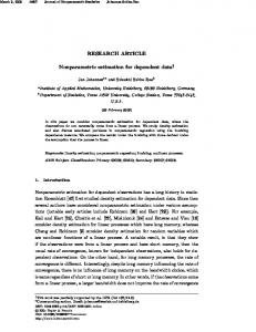
FIG. 4. 共a兲 Synthetic test two-dimensional density whose entropy, 97.8 J K−1 mol−1, was computed numerically by integrating on a grid. 共b兲 5000 points drawn according to this density function were used to estimate an entropy of 97.2 J K−1 mol−1.

For the TI between the systems given by Vs 共start兲 and V f 共end兲, 18 intermediate steps Vi共␭兲 = ␭Vs + 共1 − ␭兲V f , i = 1 , . . . , 18 were used, and the intermediate values of ␭i = 0, 1e-6, 5e-6, 1e-5, 5e-4, 1e-4, 1e-3, 1e-2, 2e-2, 3e-2, 5e-2, 7e-2, 9e-2, 0.1, 0.2, 0.3, 0.4, 0.5, 0.6, 0.7, 0.8, 0.9, 1 were distributed unevenly to obtain approximately balanced ⌬Ai values. For each value of ␭ a trajectory of 12.5 ns 共alkanes兲 or 100 ns 共dialanine兲, respectively, was generated. C. Efficient implementation

To compute the entropy via g-NN 共Eq. 共11兲兲 as described is computationally more expensive than for k-NN 共Eq. 共7兲兲, because to solve Eq. 共9兲 until convergence requires a large number of iterations. Note, however, that the density estimate Eq. 共10兲 is for all practical purposes invariant for small changes of k, because both k and ␴i,k appear in Eq. 共10兲 and scale similarly. Accordingly, convergence of k to 10% was considered sufficient to achieve accurate results, thus drastically reducing computational cost to a level similar to k-NN. The kd-tree implementation of the nearest-neighbor library ANN 关34兴 has been used for fast look-up of the k neighboring sample points. IV. RESULTS AND DISCUSSION A. Example: Simple density distributions

In a first step, our nonparametric entropy estimation was tested with synthetic probability density distributions whose entropy is accessible either analytically 共e.g., Gaussians兲 or through grid-based numerical approximation 共e.g., densities in two- and three-dimensional space兲. Figure 4 shows one of several test densities which were designed to exhibit typical features, e.g., a curved “thread,” also seen in the configurational densities of macromolecules. All reference entropies were reproduced by the estimator to within 1 J K−1 mol−1 or better 共results not shown兲. A similar test density was studied in three dimensions, as well as 42-dimensional checkerboardlike densities. In Sec. II C 3, we derived an empirical relationship of the entropy overestimation due to the smoothing of the soft degrees and the average width of the estimation kernel. Here we show that this can exploited to correct for excess smooth-

FIG. 5. Effect of the empirical smoothing correction described in the text. 共a兲 Systematic overestimation seen as deviations from the diagonal. Black crosses: uncorrected values; gray circles: corrected values. 共b兲 The same data as a function of dimensionality.

ing in more challenging high-dimensional cases, where this effect is aggravated due to increased surface effects. We considered Gaussian densities ranging from 12 to 42 dimensions. Figure 5共a兲 shows analytically computed reference entropies Sana versus values obtained from our density estimator, both with 共gray circles兲 and without 共black crosses兲 empirical smoothing correction. Figure 5共b兲 shows the same data as a function of dimensionality. As can be seen, the correction improves the obtained entropy values considerably and provides accurate values independent of dimensionality. In contrast, the uncorrected values systematically overestimate the entropy with increasing dimension. Note, that this correction is different from the QM correction described in Sec. II C 2. The empirical smoothing correction accounts for an excess of smoothing of the soft degrees of freedom, whereas the QM correction enforces a minimum of smoothing for the otherwise unphysical sharp stiff degrees of freedom. B. Example: Alkanes

We next applied our estimation method to a number of more realistic molecular test systems. Here, the accuracy of the estimate may be affected by two sampling effects; first, insufficient simulation sampling due to unvisited configurational space regions, second, locally too sparse sampling, which affects the accuracy of the NN density estimates. These two sampling effects are largely independent; whereas the sparse sampling problem, also called the “curse of dimensionality” 关14兴, aggravates with increasing dimensionality and is largely independent of the particular system studied, the simulation sampling problem will depend on the size of the accessible configurational space as well as the slowest relaxation times of that system. Consider, for example, a single harmonic well. Whereas there is no simulation sampling problem for high-dimensional wells, NN-density estimations will inevitably suffer from sparse sampling for highdimensional wells—a problem which, due to the regularization assumptions, is much less pronounced for the quasiharmonic approximation. As test systems we chose 共i兲 n-alkanes ranging from butane to decane, as a model of protein sidechain behavior, and

011913-6

PHYSICAL REVIEW E 80, 011913 共2009兲

ADAPTIVE ANISOTROPIC KERNELS FOR…

Sdir/STI

1.1 1

600

3

10

5

10

7

10

no. of sample points

STI

500

S

S (J mol−1 K−1)

S (Jmol−1K−1)

700

1.2

QH

400

SMCSA S

nc

300

Sdir Siso

200 4

5

6

7 8 no. of atoms

S

a) 400 K

pentane hexane heptane octane nonane decane

1.3

S (J mol−1 K−1)

800

9

QH

1500

S

nc

S

MCSA

S

1000

dir

S

TI

500 1500

b) 300 K

1000

500 2

10

10

FIG. 6. Entropies for the n-alcanes from butane 共N = 4兲 to decane 共N = 10兲. Sdir: direct adaptive kernel density estimation without any subspace clustering; Snc: such as Sdir but without empirical smoothing correction 共Sec. II C 3兲; Siso: direct isotropic kernel density estimation without any subspace clustering; SMCSA: sum of density estimates after subspace clustering; clust: size of largest cluster; SQH: entropy estimate according to quasiharmonic approximation. The errors of respectively Sdir, Snc, Siso, and SMCSA were below 0.23 J mol−1 K−1 in all cases and not shown in the figure, since they are smaller than the symbols. The inset shows the same data as the relative derivation to the reference TI value, indicating convergence behavior.

共ii兲 dialanine, as a minimal model for a protein backbone. The flexible wormlike shape of alkanes is likely to aggravate the two sampling problems discussed above sufficiently to explore the limits of our density estimator. To obtain reference entropy values for these systems, a thermodynamic integration scheme was used which gradually perturbed the systems toward an analytically tractable state consisting of noninteracting particles in harmonic wells, as described in methods, Sec. III B. In each case, convergence was reached 共data not shown兲. The seven n-alkanes ranging from butane to decane were described by a united-atom force field, such that the systems comprised four to ten atoms, respectively. Figure 6 shows the entropies obtained with density estimation for these systems 关35兴 as well as the reference obtained by thermodynamic integration and the QH entropy for comparison. Each of the listed density estimates has been obtained by averaging five independent trajectories. As can be seen, the QH entropy 共dashed line兲 overestimates the configurational entropy by a wide margin for all systems 共15–50%兲. The adaptive kernel density estimation, in contrast, yielded considerably improved results. For butane to octane, a deviation below 3% deviation from reference was achieved. For the largest alkanes considered, nonane and decane, a slightly reduced accuracy of 5 and 10%, respectively, was obtained. It is instructive to consider the density estimation results for the conventional isotropic kernels, Siso, also listed in the supplementary material 关35兴. Here, apparently due to the curse of dimensionality 关14兴, drastic overestimates are seen for all alkanes. For butane 共12 degrees of freedom兲 the entropy is overestimated by 9%, and for decane performs even worse than the QH approximation.

iso

S

4

10 no. of sample points

FIG. 7. Calculated dialanine entropies vs number of used sample points. 共a兲 Simulation at 400 K and, respectively, 共b兲 at 300 K The entropy labels shown are those defined in the caption of Fig. 6.

This result shows that it is the adaptive anisotropic kernels 共ellipsoids rather than spheres, whose principal axes are determined from the local density by a principal component analysis, cf. methods兲, which provide the observed accuracy. Anisotropic kernels according to Eq. 共14兲 rather than according to Eq. 共13兲 turned out to yield more accurate results 共data for the latter not shown兲. As can also be seen in the figure, the empirical smoothing correction, which accounts for the inevitable blurring during the averaging process of the density estimation 共Sec. II C 3兲, markedly improved the density estimates. The inset of Fig. 6 highlights the convergence behavior of the adaptive anisotropic kernel estimates for alkanes with increasing simulation length. Clear convergence is seen for all alkanes up to octane, i.e., up to 24-dimensional densities. Whereas for these alkanes, 500.000 sample points sufficed for an accurate density estimate, 5.000.000 were required for nonane, and even more for decane, where sufficient sampling was not reached. In all cases, four sample points per picosecond simulation time were recorded. Although it is unclear at this point whether this lack of convergence is due to insufficient sampling of the simulation or the curse of dimensionality due to sparse sampling described above, the high flexibility of decane suggests the former. In the next section, we will address this question by considering a less flexible, but larger system. C. Example: Dialanine

Dialanine, as a minimal model of a protein backbone comprising 45 atoms, served as our largest test system. The molecule was simulated with implicit solvent at temperatures 300 and 400 K using a united-atom force field. Figure 7 shows entropies Sdir and SQH obtained for simulation lengths ranging from 100 ps to 500 ns. The TI reference entropy is shown as a horizontal line. Similarly as seen above for the alkanes, the QH entropy SQH overestimates the TI reference. Interestingly, and in contrast to the other estimates, the QH-

011913-7

PHYSICAL REVIEW E 80, 011913 共2009兲

HENSEN, GRUBMÜLLER, AND LANGE

D. Application: Coldshock protein

The previous sections established that adaptive anisotropic kernel density estimation is very well feasible in configurational space of up to 45 dimensions. Although this is still far from the high dimensionality typically found for biological macromolecules, it holds the promise to provide the missing building block for a reliable application of the minimally coupled subspace framework 共MCSA兲 derived in detail in Ref. 关15兴. Briefly, full correlation analysis 关20兴 共FCA兲 is used to obtain nearly independent orthogonal configurational subspaces, which allow to approximately factorize the configurational space density. Subsequently, adaptive anisotropic kernels are used to estimate the entropy contributions for each of these subspaces. To test the feasibility and accuracy of this approach, we apply this framework to the coldshock protein, a 67-residue soluble protein 共protein database entry 1CSP兲 which was simulated in explicit solvent, as described in methods. Of particular interest was the question of how many 共soft兲 degrees of freedom should be subjected to FCA and to the adaptive anisotropic kernel density estimation, leaving the remaining 共stiff兲 degrees of freedom to the Schlitter QH approximation. For simplicity and computational efficiency, only backbone contributions to the configurational entropy were considered. FCA was carried out on the first

3200

S

MCSA

S

3000

tot

S

tot,QH

2800 2600

0

10

2400

eigenvalue

−1

−1

S (JK mol )

estimate error increases with the length of the simulation. As a consequence, the longest, 500 ns, trajectory yields the most inaccurate result with an error of 250%. We attribute this peculiar behavior to a decreasing quality of the harmonic approximation with increasing complexity of the sampled configurational space. In contrast, the entropy obtained with density estimation Sdir converges toward the correct value with increasing simulation length. For the 500 ns simulation, the TI reference is reached to within 4.0 and 18% for 400 and 300 K, respectively. Again, density estimates from isotropic kernels yielded even lower accuracy than the QH estimate in all cases. Further, compared to the alkanes, the smoothing correction improved density estimates to an even larger extent; the uncorrected estimates overestimated the reference by 16 and 33% for 400 and 300 K, respectively. This result corroborates the previous observation that the achieved accuracy was mainly due to the adaptive anisotropic kernels. Moreover, even though the dimension of the configurational space of dialanine is almost twice as large as that of nonane, the obtained accuracy is similar despite the fact that ten times less sample points were used for dialanine. Apparently, the curse of dimensionality is not yet severe here, thus underscoring the robustness of the adaptive anisotropic kernels even for high dimensionality. A second conclusion is that, as expected, lack of simulation sampling limited the accuracy of the decan entropy estimates. This interpretation is further supported by the fact that more accurate estimates are obtained for the high-temperature simulations, which are likely to provide enhanced simulation sampling, but sparser local sampling. In this sense, alkanes proved to be particular hard test systems.

2200

−5

10

2000 −10

10

1800 100

200

0

200 400 mode index

300 mode index

400

600

500

FIG. 8. Estimated entropies for the coldshock protein 共1CSP, backbone only兲. The total estimate, Stot, as a function of MCSA subspace size 共100, . . . , 500 modes兲, was calculated as sum of SMCSA, the estimate obtained by application of adaptive anisotropic kernels to minimally coupled subspaces obtained by FCA, and the QH estimate for the remaining modes, as described in the text; SPCA: cumulative QH estimate; Stot,QH: global QH reference.

100, 200, . . . , 500 modes of the configurational ensemble, and nearly noncorrelated subspaces were defined as described in Ref. 关15兴. Our adaptive anisotropic kernel estimate was subsequently applied to each of the resulting minimally coupled subspaces yielding an improved entropy estimate SMCSA. The remaining modes were considered via the Schlitter QH approximation, Eq. 共6兲. The sum of these two yields the desired entropy estimate Stot, also shown in Fig. 8. Due to the large size of this protein no converged TI entropy reference could be obtained; hence, we here resort to comparison with the QH estimate of the total configurational space density Stot,QH. Figure 8 shows that the combination of FCA and adaptive anisotropic kernels improves on the QH estimate in all cases. In particular, a marked improvement on the QH estimate is seen for the adaptive anisotropic kernel estimate, which shows that the neglect of nonlinear and higher-order correlations, and of anharmonicities by the established QH method implies an overestimation of the entropy by at least 14% 共QH: 3081 J K−1 mol−1 vs SFCA: 2710 J K−1 mol−1兲. It turns out that for the coldshock protein 400 modes need to be subjected to the minimally coupled subspace approach for converged results. Obviously only the 200 stiffest modest are already sufficiently decoupled by PCA and can be well approximated by a quasiharmonic density. This empirical distinction between stiff and soft modes is nicely reflected in the eigenvalue spectrum shown in the inset of Fig. 8. Whereas eigenvalues of modes 1 to 400 decrease smoothly, an abrupt drop is seen at mode 400. Similar observations for calmodulin 关15兴 suggest that such abrupt drop can be used to identify the stiff modes that can be subjected to the QH approximation. Our results also suggest that, generally, a large fraction of degrees of freedom needs to be subjected to MCSA to obtain reliable estimates.

011913-8

PHYSICAL REVIEW E 80, 011913 共2009兲

ADAPTIVE ANISOTROPIC KERNELS FOR… V. CONCLUSIONS

come the three limitations inherent in the conventional quasiharmonic approximation, i.e., neglect of nonlinear and higher-order correlations, of anharmonicity, and of multimodality. So far we have applied the method to the proteins insulin 共51 residues兲 and calmodulin 共146 residues兲. In both cases the method yielded significantly lower entropy than QH and was able to reconcile experimental data previously found to be inconsistent with the QH entropy. Although encouraging, further studies will have to corroborate these results, and investigate possible limitations in more detail.

We have introduced a kernel-based density estimation method and showed that it provides accurate results in even the high-dimensional and quite complex configurational space density generated by the dynamics of biological macromolecules. Whereas established k-nearest-neighbor estimators have been reported to fail to converge for 23dimensional configurational space with 15 million sample points, the adaptive anisotropic kernels developed here provide robust results in up to 45 dimensions with only 500.000 sample points. We attribute this improvement to the occurrence of typically sparsely sampled configurational density “threads” ubiquitous in protein dynamics, to which, apparently, our locally multivariate approach provides enhanced approximation. Used within the framework of the minimally coupled subspace approach 关15兴, this density estimator serves to over-

U.H. was supported by the Deutsche Forschungsgemeinschaft 共research training group 782兲. O.F.L. was supported by the Human Frontiers of Science Foundation

关1兴 S. Cheluvaraja and H. Meirovitch, Proc. Natl. Acad. Sci. U.S.A. 101, 9241 共2004兲. 关2兴 S. Cheluvaraja and H. Meirovitch, J. Chem. Phys. 125, 024905 共2006兲. 关3兴 T. P. Straatsma and J. A. McCammon, Annu. Rev. Phys. Chem. 43, 407 共1992兲. 关4兴 C. Peter, C. Oostenbrink, A. van Dorp, and W. F. van Gunsteren, J. Chem. Phys. 120, 2652 共2004兲. 关5兴 D. L. Beveridge and F. M. DiCapua, Annu. Rev. Biophys. Biophys. Chem. 18, 431 共1989兲. 关6兴 P. Kollman, Chem. Rev. 93, 2395 共1993兲. 关7兴 H. Schäfer, A. E. Mark, and W. F. van Gunsteren, J. Chem. Phys. 113, 7809 共2000兲. 关8兴 H. Meirovitch, Curr. Opin. Struct. Biol. 17, 181 共2007兲. 关9兴 J. N. Karplus and Martin Kushick, Macromolecules 14, 325 共1981兲. 关10兴 J. Schlitter, Chem. Phys. Lett. 215, 617 共1993兲. 关11兴 C. Chang, W. Chen, and M. Gilson, J. Chem. Theory Comput. 1, 1017 共2005兲. 关12兴 R. Baron, W. van Gunsteren, and P. Hünenberger, Trends Chem. Phys. 11, 87 共2006兲. 关13兴 R. Baron, A. deVries, P. Hünenberger, and W. van Gunsteren, J. Phys. Chem. B 110, 8464 共2006兲. 关14兴 R. E. Bellman, Adaptive Control Processes 共Princeton University Press, Princeton, NJ, 1961兲. 关15兴 U. Hensen, H. Grubmüller, and O. F. Lange 共unpublished兲. 关16兴 H. Matsuda, Phys. Rev. E 62, 3096 共2000兲. 关17兴 A. Baranyai and D. J. Evans, Phys. Rev. A 40, 3817 共1989兲. 关18兴 L. Comtet, Advanced Combinatorics: The Art of Finite and Infinite Expansions 共Reidel, Dordrecht, Boston, 1974兲, Vol. 1. 关19兴 V. Hnizdo, E. Darian, A. Fedorowicz, E. Demchuk, S. Li, and H. Singh, J. Comput. Chem. 28, 655 共2007兲.

关20兴 O. F. Lange and H. Grubmüller, Proteins 70, 1294 共2008兲. 关21兴 J. Haas, E. Vöhringer-Martinez, A. Bögehold, D. Matthes, U. Hensen, A. Pelah, B. Abel, and H. Grubmüller, ChemBioChem 10, 1816 共2009兲. 关22兴 N. Go and H. A. Scheraga, J. Chem. Phys. 51, 4751 共1969兲. 关23兴 G. Kaminski, R. Friesner, J. Tirado-Rives, and W. Jorgensen, J. Phys. Chem. B 105, 6474 共2001兲. 关24兴 R. O. Duda, P. E. Hart, and D. G. Stork, Pattern Classification, 2nd ed. 共Wiley-Interscience, New York, 2000兲. 关25兴 A. W. Schüttelkopf and D. M. F. van Aalten, Acta Crystallogr., Sect. D: Biol. Crystallogr. 60, 1355 共2004兲. 关26兴 W. F. van Gunsteren, X. Daura, and A. E. Mark, GROMOS Force Field 共1998兲, pp. 1211–1216. 关27兴 D. Van Der Spoel, E. Lindahl, B. Hess, G. Groenhof, A. E. Mark, and H. J. C. Berendsen, J. Comput. Chem. 26, 1701 共2005兲. 关28兴 W. L. Jorgensen, J. Chandrasekhar, J. D. Madura, R. W. Impey, and M. L. Klein, J. Chem. Phys. 79, 926 共1983兲. 关29兴 H. J. C. Berendsen, J. P. M. Postma, W. F. van Gunsteren, A. DiNola, and J. R. Haak, J. Chem. Phys. 81, 3684 共1984兲. 关30兴 B. Hess, H. Bekker, H. J. C. Berendsen, and J. G. E. M. Fraaije, J. Comput. Chem. 18, 1463 共1997兲. 关31兴 S. Miyamoto and P. A. Kollman, J. Comput. Chem. 13, 952 共1992兲. 关32兴 T. Darden, D. York, and L. Pedersen, J. Chem. Phys. 98, 10089 共1993兲. 关33兴 M. Tyka, A. Clarke, and R. Sessions, J. Phys. Chem. B 110, 17212 共2006兲. 关34兴 URL http://www.cs.umd.edu/~mount/ANN/. 关35兴 See EPAPS Document No. E-PLEEE8-80-094907 for detailed test results. For more information on EPAPS, see http:// www.aip.org/pubservs/epaps.html.

ACKNOWLEDGMENTS

011913-9