Adaptive Behaviour Based Robotics using On-Board Genetic ...

Adaptive Behaviour Based Robotics using On-Board Genetic Programming

Anders Kofod-Petersen

For the degree of Cand. Scient. Norwegian University of Science and Technology 2002

i

Abstract This thesis investigates the use of Genetic Programming (GP) to evolve controllers for an autonomous robot. GP is a type of Genetic Algorithm (GA) using the Darwinian idea of natural selection and genetic recombination, where the individuals most often is represented as a tree-structure. The GP is used to evolve a population of possible solutions over many generations to solve problems. The most common approach used today, to develop controllers for autonomous robots, is to employ a GA to evolve an Artificial Neural Network (ANN). This approach is most often used in simulation only or in conjunction with online evolution; where simulation still covers the largest part of the process. The GP has been largely neglected in Behaviour Based Robotics (BBR). The is primarily due to the problem of speed, which is the biggest curse of any standard GP. The main contribution of this thesis is the approach of using a linear representation of the GP in online evolution, and to establish whether or not the GP is feasible in this situation. Since this is not a comparison with other methods, only a demonstration of the possibilities with GP, there is no need for testing the particular test cases with other methods. The work in this thesis builds upon the work by Wolfgang Banzhaf and Peter Nordin, and therefor a comparison with their work will be done.

ii

Acknowledgements I would like to thank Asbjørn Thomasen and Trond Kandal for their invaluable help with the C programming. Wolfgang Banzhaf for pointers and good suggestions for improvement. Gorm Andersen for his assistance with the experiments. And, last but not least, my supervisor Keith Downing for his patience with me.

Contents I

Introduction

1

1 Introduction 1.1 Motivation . . . . . . . . . . . . . . . . . . . . . . . . . . . . . . . . 1.2 Layout of the thesis . . . . . . . . . . . . . . . . . . . . . . . . . . .

3 4 4

II

5

Theory and Approach

2 Theory 2.1 Introduction . . . . . . . . . . . . . . . . 2.2 Behaviour Based Robotics . . . . . . . . 2.2.1 Introduction . . . . . . . . . . . . Behaviour based on neuroscience Behaviour based on psychology . Behaviour based on ethology . . . 2.2.2 Behaviour in robot . . . . . . . . 2.2.3 Behaviour based architectures . . 2.2.4 Adaptive behaviour . . . . . . . . Adaptive individuals – learning . Reinforced learning . . . . Fuzzy control . . . . . . . Artificial Neural Networks Adaptive populations – evolution 2.2.5 Summary . . . . . . . . . . . . . 2.3 Genetic Programming . . . . . . . . . . . 2.3.1 Introduction . . . . . . . . . . . . 2.3.2 Definition . . . . . . . . . . . . . 2.3.3 Genetic programming basics . . . Terminals and functions . . . . . Fitness and selection . . . . . . . Mutations . . . . . . . . . . . . . Crossover . . . . . . . . . . . . . Asexual reproduction . . . . . . . 2.3.4 Summary . . . . . . . . . . . . . iii

. . . . . . . . . . . . . . . . . . . . . . . . .

. . . . . . . . . . . . . . . . . . . . . . . . .

. . . . . . . . . . . . . . . . . . . . . . . . .

. . . . . . . . . . . . . . . . . . . . . . . . .

. . . . . . . . . . . . . . . . . . . . . . . . .

. . . . . . . . . . . . . . . . . . . . . . . . .

. . . . . . . . . . . . . . . . . . . . . . . . .

. . . . . . . . . . . . . . . . . . . . . . . . .

. . . . . . . . . . . . . . . . . . . . . . . . .

. . . . . . . . . . . . . . . . . . . . . . . . .

. . . . . . . . . . . . . . . . . . . . . . . . .

. . . . . . . . . . . . . . . . . . . . . . . . .

. . . . . . . . . . . . . . . . . . . . . . . . .

. . . . . . . . . . . . . . . . . . . . . . . . .

. . . . . . . . . . . . . . . . . . . . . . . . .

7 7 7 7 8 8 9 9 10 10 11 11 11 11 13 14 14 14 14 15 15 15 17 17 18 18

CONTENTS

iv 3 Related Work 3.1 Introduction . . . . . . . . . . . 3.2 Work with genetic algorithms . . 3.2.1 Introduction . . . . . . . 3.2.2 Simulation . . . . . . . 3.2.3 On-board . . . . . . . . 3.2.4 Hybrid . . . . . . . . . 3.3 Work with genetic programming 3.3.1 Introduction . . . . . . . 3.3.2 Simulation . . . . . . . 3.3.3 On-Board . . . . . . . . Introduction . . . . . . . Basic model . . . . . . . ADF model . . . . . . . 3.3.4 Hybrid . . . . . . . . . 3.4 Summary . . . . . . . . . . . .

. . . . . . . . . . . . . . .

. . . . . . . . . . . . . . .

. . . . . . . . . . . . . . .

. . . . . . . . . . . . . . .

. . . . . . . . . . . . . . .

. . . . . . . . . . . . . . .

. . . . . . . . . . . . . . .

. . . . . . . . . . . . . . .

. . . . . . . . . . . . . . .

. . . . . . . . . . . . . . .

. . . . . . . . . . . . . . .

. . . . . . . . . . . . . . .

. . . . . . . . . . . . . . .

. . . . . . . . . . . . . . .

. . . . . . . . . . . . . . .

. . . . . . . . . . . . . . .

. . . . . . . . . . . . . . .

. . . . . . . . . . . . . . .

. . . . . . . . . . . . . . .

. . . . . . . . . . . . . . .

19 19 19 19 20 21 22 22 22 23 24 24 25 26 27 27

4 Approach 4.1 Introduction . . . . . . . . . . 4.2 The Khepera . . . . . . . . . . 4.3 Genetic programming structure 4.3.1 Individuals . . . . . . 4.3.2 Reproduction . . . . . Selection . . . . . . . Crossover . . . . . . . Mutation . . . . . . .

. . . . . . . .

. . . . . . . .

. . . . . . . .

. . . . . . . .

. . . . . . . .

. . . . . . . .

. . . . . . . .

. . . . . . . .

. . . . . . . .

. . . . . . . .

. . . . . . . .

. . . . . . . .

. . . . . . . .

. . . . . . . .

. . . . . . . .

. . . . . . . .

. . . . . . . .

. . . . . . . .

. . . . . . . .

. . . . . . . .

29 29 29 30 32 33 34 34 35

. . . . . . . .

III Results and Evaluation 5 Results 5.1 Introduction . . . . . . . . . . . . . . . . . . . . 5.2 General settings . . . . . . . . . . . . . . . . . . 5.2.1 Function set . . . . . . . . . . . . . . . . 5.2.2 Terminal set . . . . . . . . . . . . . . . . 5.2.3 Selection, crossover, and mutation . . . . 5.3 Test run . . . . . . . . . . . . . . . . . . . . . . 5.3.1 Upside down . . . . . . . . . . . . . . . 5.3.2 Correct orientation . . . . . . . . . . . . 5.4 Obstacle avoidance . . . . . . . . . . . . . . . . 5.4.1 Test case 1 - The population way . . . . . 5.4.2 Result . . . . . . . . . . . . . . . . . . . 5.4.3 Test case 2 - The individual way . . . . . 5.4.4 Result . . . . . . . . . . . . . . . . . . . 5.5 Comparison . . . . . . . . . . . . . . . . . . . . 5.5.1 Introduction . . . . . . . . . . . . . . . . 5.5.2 Comparison between the two experiments Verification . . . . . . . . . . . . . . . . Individual vs. population solution . . . . Performance . . . . . . . . . . . . . . .

37 . . . . . . . . . . . . . . . . . . .

. . . . . . . . . . . . . . . . . . .

. . . . . . . . . . . . . . . . . . .

. . . . . . . . . . . . . . . . . . .

. . . . . . . . . . . . . . . . . . .

. . . . . . . . . . . . . . . . . . .

. . . . . . . . . . . . . . . . . . .

. . . . . . . . . . . . . . . . . . .

. . . . . . . . . . . . . . . . . . .

. . . . . . . . . . . . . . . . . . .

. . . . . . . . . . . . . . . . . . .

39 39 39 40 41 41 41 42 43 43 44 44 45 46 48 48 48 49 49 49

CONTENTS 5.5.3

v Comparison between this work and others . . . . . . . . . . .

6 Discussion 6.1 Introduction . . . 6.2 Summary . . . . 6.3 The research area 6.4 Robots . . . . . . 6.5 Future work . . .

. . . . .

. . . . .

. . . . .

. . . . .

. . . . .

. . . . .

. . . . .

. . . . .

. . . . .

. . . . .

. . . . .

. . . . .

. . . . .

. . . . .

. . . . .

. . . . .

. . . . .

. . . . .

. . . . .

. . . . .

. . . . .

. . . . .

. . . . .

. . . . .

. . . . .

. . . . .

. . . . .

. . . . .

50 51 51 51 52 52 53

Bibliography

53

IV

61

Appendices

A Code A.1 Header file . . . . . . . . . . . . . . . . . . . . . . . . . . . . . . . . A.2 Main code . . . . . . . . . . . . . . . . . . . . . . . . . . . . . . . .

63 63 71

vi

CONTENTS

List of Figures 2.1

Overview of a GP tree structure . . . . . . . . . . . . . . . . . . . .

16

4.1 4.2 4.3 4.4 4.5

The Khepera robot . . . . . . . . . . Overview of the framework . . . . . . Systems execution cycle . . . . . . . Overview of the individuals structure . Example of crossover . . . . . . . . .

. . . . .

. . . . .

. . . . .

. . . . .

. . . . .

. . . . .

. . . . .

. . . . .

. . . . .

. . . . .

. . . . .

29 30 31 32 34

5.1 5.2 5.3 5.4 5.5 5.6 5.7 5.8 5.9 5.10 5.11 5.12

Fitness graph for first test run . . . . . . . . . . . . Fitness and collisions graphs for second test run . . Population first run . . . . . . . . . . . . . . . . . Population second run . . . . . . . . . . . . . . . . Population third run . . . . . . . . . . . . . . . . . Population average . . . . . . . . . . . . . . . . . Three stages of behaviour . . . . . . . . . . . . . . Individual first run . . . . . . . . . . . . . . . . . Individual second run . . . . . . . . . . . . . . . . Individual third run . . . . . . . . . . . . . . . . . Individual average . . . . . . . . . . . . . . . . . . Average number of collisions for both experiments

. . . . . . . . . . . .

. . . . . . . . . . . .

. . . . . . . . . . . .

. . . . . . . . . . . .

. . . . . . . . . . . .

. . . . . . . . . . . .

. . . . . . . . . . . .

. . . . . . . . . . . .

. . . . . . . . . . . .

. . . . . . . . . . . .

42 43 45 45 45 45 46 47 47 47 47 48

vii

. . . . .

. . . . .

. . . . .

. . . . .

. . . . .

. . . . .

viii

LIST OF FIGURES

Part I

Introduction

1

Chapter 1

Introduction The most exciting phrase to hear in science, the one that heralds the most discoveries, is not ”Eureka!”, but ”That’s funny...” – Isaac Asimov Within the last decade a huge amount of work has been made in the field of Behaviour Based Robotics (BBR). Up until the mid-1980s the majority of work was based on the sense-plan-act paradigm. At this time Rodney Brooks developed his subsumption architecture, which is a purely reactive behaviour based method. As a result of Brooks work on BBR, the research in the later years have been mostly concentrated on the reactive behaviour, and less on the sense-plan-act paradigm; the later haven’t completely vanished, since a lot of work is still done in the field of Reinforced learning. For the last decade most of the research on BBR has been concentrated on using some kind of Artificial Neural Network (ANN) to control a robot. This has either been pure ANNs or ANNs in conjunction with some kind of Evolutionary Method (EM). Most of the work on BBR have been directed towards the use of simulation, even though lately some focusing have been done on the use of simulation and on-board evolution simultaneous, and some work have been done on on-board evolution only. One major approach within the field of EM has been largely neglected. Namely the field of Genetic Programming (GP). This is largely because of the time this method consumes when running, and some have argued that level at which a GP operates is not low enough. Some work has been done in trying to use GP to generate ANNs for controlling a robot, most of this work, however, has been done in simulation and then tested on the real robot. Recently some work from Peter Nordin and Wolfgang Banzhaf has explored the possibilities of using a variation of the GP to evolve controllers for the Khepera robot on-board [NB95]. 3

4

CHAPTER 1. INTRODUCTION

1.1 Motivation Robots, or agents, working in the real world is faced with the problem of a very open domain; it is often hard to know any thing about the dynamics of the real world. This uncertainty leads us, according to Brooks [Bro87] and others, for an example see [BG92], [HHC 96], to the pragmatic view that reactive behaviour is more suited to “survival” than the more conservative sense-plan-act paradigm; as used by Nilson [Nil84]. The subsumption theory is not the only way of achieving a reactive behaviour. Several interesting approaches have emerged in the last decade. One of the most promising “bottom-up” approaches today is the use of an EM, often in conjunction with ANNs, to generate the controller for a particular robot and its task. The motivation for this work can be divided into two major parts: first, the lack of GP in todays BBR, and secondly the problem of simulation, where it is very hard to construct a simulator which somehow mimic the world in any useful way. This work will try to show that it is possible, and feasible, to use a GP running on-board on the robot.

1.2 Layout of the thesis This thesis is organised into tree pieces. First the theory and background to support this work will be covered. The design choices and implementation will be described. Secondly, the implementation will be tested on obstacle avoidance. Last, but not least, it will try to draw some conclusions based on the work presented here.

Part II

Theory and Approach

5

Chapter 2

Theory The science of today is the technology of tomorrow. – Edward Teller

2.1 Introduction This chapter will first cover the theory of behaviour based robotics, it will then describe an overview of the Genetic programming theory, and finally it will describe and discuss the pros and cons of on-board evolution.

2.2 Behaviour Based Robotics This part will briefly cover a definition of intelligence; it will then describe what behaviour in animals is, and how it can inspire the use of behaviour based (artificial) systems, covering the more theoretical part first, and then the engineering view. Then a few behaviour based architectures will be covered; with a discussion of adaptive behaviour to follow.

2.2.1 Introduction Before the topic can be covered in any meaningful way, some definition of robots and intelligence must be agreed upon. This work will adapt the definition stated by Arkin ([Ark98]). An intelligent robot is a machine able to extract information from its environment and use knowledge about its world to move safely in a meaningful and purposive manner. Furthermore some kind of framework for the classification of behaviour is required. The science of behaviour can be classified into three major fields † ; neuroscience, psychology, and ethology. † Not

exclusive in any way, and definitely overlapping

7

CHAPTER 2. THEORY

8 Behaviour based on neuroscience

From the field of neuroscience the study of the central nervous system (CNS), and the brains of humans and other animals has resulted in a number of theories concerning behaviour and the brain. The brain of any mammal consists of three major parts: the fore brain, the brain stem, and the spinal cord. The fore brain includes, among other things, the limbic system, which provides the basic behavioural survival responses; Thalamus, which processes incoming sensory information and outgoing motor activity; and Hypothalamus, which controls homeostasis. The later is the place which is most often associated with what is called behaviour based systems. The brain stem includes, the mid brain, which processes incoming sensory information, and controls primitive motor response systems; the hind brain, which consists of the pons; the cerebellum; and the medulla oblongata, which connects the brain to the spinal cord. The spinal cord is the reflexive pathway which is use for controlling the different motor systems. For a more thorough discussion of the brain see for an example: [GIM98]. Behaviour based on psychology Psychology has historically focused more on the functions of the mind as opposed to the functions of the brain. The two most interesting fields within psychology, at least from the perspective of behaviour based robotics, is probably behaviourism and ecological psychology. Behaviourism was founded by John B. Watson in 1913, as a reaction to the psychology of his time, which was primarily based on introspection. Watson argued that almost all behaviour is a result of conditioning, and that the environment shapes our behaviours by reinforcing habits† . The behaviourists based their theories on the stimuliresponse paradigm, which states that to any stimulus some kind of response will be the result. Ecological psychology owes a great deal to the American psychologist J. J. Gibson. He suggests a high correlation between the organism, it’s environment, and how evolution affects it’s development. In Gibson’s own words: The word “animal” and “environment” make an inseparable pair. Each term implies the other. No animal could exist without an environment surrounding it. Equally, though not so obvious, an environment implies an animal (or at least an organism) to be surrounded. [Gib79] Gibson was mostly concerned with the theories of visual perception, both in animals and humans. From his theories spring forth the two concepts of (in the terms of Brooks [Bro91]) situatedness, the robot (organism) is situated and surrounded by the real world; and embodiment, a robot (organism) has a real physical form. † Perhaps

one of the most known examples of this approach is Pavlov’s dogs.

2.2. BEHAVIOUR BASED ROBOTICS

9

Behaviour based on ethology Ethology is the study of animals behaviour in their natural environment, or as Niko Tinbergen puts is “the biological study of behaviour”. Tinberg focused on four primary behaviour areas: i) causation, which is the study of those outside influences and internal states that lead animals to specific behaviour; ii) survival value, which is pretty much self explanatory; iii) development, which springs from the the controversy between comparative psychologist and ethologists, where the psychologists concentrated on nurture as opposed to the ethologists who stressed the importance of nature; iv) evolution, where ethology borders genetics, evolutionary biology, and ecology. For a more thorough introduction to ethology see [Sla85].

2.2.2 Behaviour in robot Behaviour in robots comes in a broad spectrum. From the purely reactive, or reflexive; to the very deliberate. This work will lean heavily on the part of the spectrum concerning reactive behaviour. The simplest way to view behaviour in robotics is to adopt the position advocated by behaviourists, that to each stimulus some reaction exists. In this view behaviour is seen as basic building blocks for actions. Probably the most famous example of this approach is Braitenberg’s vehicles [Bra84]. The behaviouristic approach to robotics grows from the recognition that planning is often a waste of time; especial in a highly dynamical world, i.e. the real world [Bro87]. The reactive system, or reflexes, avoids the use of explicit abstract knowledge about the world which the robot inhabits. Since the construction of abstract world models can be very time consuming, this approach is very valuable in very dynamic and/or hazardous worlds. Three key concepts of the reactive view on behaviour emerges. Namely, situatedness and embodiment, which already has been discussed i section 2.2.1, and the third emergence, which states that intelligence arises from the interaction between the robot and the environment [Bro91]. The major issue in behaviour base robotics is where do behaviour come from? what are the right building blocks? and how do we define primitive behaviours? Several approaches has been tested throughout the short history of behaviour based robotics. Three major directions stands out: ethologically guided design, situated activity based design, and experimental driven design. In Ethologically guided design the basis is the study of animals. A model of a particular animals behaviour is found in biology. The model is modified to suit any computational, or hardware, restrictions. The experiment is then conducted, preferably on a physical robot, and any result is compared with the original biological experiment. One nice example of this approach can be found in [LWH98] where the phonotaxis of the female cricket Gryllus Bimaculatus was produced on a robot with a simple artificial neural network. The experiment was conducted under the same conditions as the biological experiment. The robot responded with phonotaxis to the calling song of real male Gryllus Bimaculatus. This work showed that phonotaxis could be achieved with a ANN much smaller than the model used when studying the real cricket. Furthermore, it showed that the close coupling between the morphological auditory matched filtering of the robot cricket, and it’s simple neural control mechanism could explain the behaviour seen in nature. The major point with this work was, not that the model of Lund et. al. is the way a real cricket works, but that this very simple model could explain the patterns seen in

CHAPTER 2. THEORY

10

nature. Other work of the same kind has been done by Miglino and Lund, where they reconstructed an well known experiment on rats, where the rats are supposed to navigate through a labyrinth. Here they also showed that there was a much more simple model than the one used by most biologists, which is based on the rat making cognitive maps of the labyrinth [LM98],[ML99]. Situated activity based design is based on the approach that whenever a robot finds itself in a new situation it chooses one appropriate action to take. This means that any problem becomes one of perception. The robot have to recognise which situation it is in to select the proper response. Experimental driven design is the “true” human bottom up approach. The principle is that one starts of with some limited amount of capabilities, test whether or not they work, debug the behaviour which does not work, add new features, and go through the loop again. One very nice example can be found in [Bro89], where a six legged robot’s ability to walk was developed. Several iterations were used, where different capabilities were added, such as force balancing, whiskers, and pitch stabilisation.

2.2.3 Behaviour based architectures The design and building of behaviour based robotic systems has lead to a great variety of types. Each with their own idiosyncrasies; yet they exhibit a lot of common features. First of all, the emphasis is on the coupling of sensory inputs to responses, as dictated by behaviourists (see section 2.2.1). Secondly, the use of sub symbolic methods is prevalent, as opposed to representational symbolic knowledge. Third, the use of decomposition is common, i.e. use of meaningful behaviour units. For a very thorough discussion of different architectures see [Ark98], and for a overview of current work in the field see [GG96].

2.2.4 Adaptive behaviour Up until now this part has covered the purely reactive robotic systems. Since reactive behaviour, or reflexes, only can help in a narrow group of problems, some kind of adaptation is needed to function in an ever changing environment. Before continuing it would be fruitful to define adaptation. According to MerriamWebster’s Collegiate Dictionary, adaptation is: Modification of an organism or its parts that makes it more fit for existence under the conditions of its environment Adaptation comes in two general flavours, a) adaptation in an individual within its own life time – learning, or b) adaptation within a population over time – evolution. This part will first cover some different methods for introducing adaptation in an individual: reinforced learning, the use of fuzzy system, and artificial neural networks. It will then describe the different approaches to applying evolution to a population of possible solutions (individuals).

2.2. BEHAVIOUR BASED ROBOTICS

11

Adaptive individuals – learning Adaptation in an individual throughout its lifetime is learning. According to MerriamWebster’s Collegiate Dictionary, learning is: Modification of a behavioral tendency by experience (as exposure to conditioning) Learning in robotic systems comes in a variety of flavours, here reinforced learning and fuzzy control will be covered briefly. Since the trend in the behaviour based robotics community has been to use ANNs, this will be cover more throughly. Reinforced learning has its roots in behaviourism and the likes of Watson and Pavlov (see section 2.2.1). For reinforced learning to work an agent (robot) has to build on a certain model. In this model an agent has a set of sensors to observe the state of its environment, and a set of actions it can perform to change the state in which the agent is. Last, not not least, the agent needs a goal. To learn the agent how to achieve it’s goal reinforcement is used. A reward is given to each distinct action the agent can perform in each distinct state. So, a reward will be given to each state-action transition which achieves the goal, and no reward to all other transitions. One of the most popular learning algorithms used today is Q learning. Since this is beyond the scope of this work, a more through description of reinforced learning can be found here [Mit97]. Examples of work done with robots and reinforced learning includes: [MB90], [Tan91], [Lin91], [MC91], and [Kae92]. Fuzzy control is based on fuzzy logic, which set itself apart from predicate logic by allowing values to be, more or less, members of different set, and not just the conventional true or false based membership. Fuzzy systems has been one of the AI worlds biggest success stories, largely due to the fact that “fuzzynes” is an integrated part of many things connected with humans; especial our language; almost everyone has used a sentence like: “This car is a bit more green than this one”. Fuzzy systems are excellent for a large group of problems, such as: maintaining an airplane in straight-and-level flight, hold the temperature of a room at 20 degrees, and dispatching elevators in a building [MF00]. Even though this approach should be well suited to solve behaviour based problems, only a few experiments has been conducted. The best known are properly the robot “Flakey” from SRI, and “MARGE” from North Carolina State University. For a more through description of fuzzy systems, see for example: [MF00]. Artificial Neural Networks was first described in 1943, where McCulloch-Pitts, inspired by neurobiology, proposed a model of neurons [MP47]. This model was based on the assumption that neuron was either on or off. This led to a network structure where the network was composed of directed unweighted edges of excitatory or inhibitory type. Each unit is also provided with a certain threshold value. Even though this kind of neuron is a very simple structure, it can been shown that all logical functions can be implemented with a McCulloch-Pitts network. Weighted networks and McCulloch-Pitts Networks are equivalent, and any finite automaton can be simulated (see [Roj96] for examples and references).

CHAPTER 2. THEORY

12

The major problem with the McCulloch-Pitts units is their lack of free parameters. Learning can only be implemented by modifying the way units are connected, and their threshold values. This lack of flexibility leads to a more complex version of ANNs. In 1958 Frank Rosenblatt proposed the Perceptron, a more general computational model that McCullochPitts units. In the 1960s The model was refined by Minsky and Papert [MP69]. The model proposed by Rosenblatt consisted of a whole network for the solution of pattern recognition problems, where the only significant difference from the McCulloch-Pitt unit was the presses of weights in the network. The learning algorithm proposed by Rosenblatt was the Perception Learning Algorithm (see equation: 2.1),
where A is the set on input
vectors where a perceptron computes the binary function f w x  1;  x  A and fw x  0;  x  B




E w 

∑

x A







1 fw x   

∑ fw

x B




x

(2.1)

This
function is defined over all of weight space and the purpose is to minimise it.
Since E w  is positive or zero, we want to reach the global minimum where E w  0. This is done by selecting a weight, by random, and then search the weight space for a
better solution, in an attempt to reduce the error function E w  in each step. Minsky and Papert modified Rosenblatt’s model. By adding the possibility of predicates in the input layer, where the value of a single input bit can be calculated. These predicates can be of any format, e.g. a simple logical function, or a large program running on a super computer. McCulloch-Pitts and Minsky-Papert was not the only ones conducting research on ANNs; But they were some of the more influential. Several others deserves to be mentioned, here I will only name two of the best known: Hebb, who described a learning paradigm. Where one of the core ideas was that the strength of synaptic connection was proportional to the correlation of pre- and post-synaptic potentials. Uttley, who in the late 50’s developed a paradigm based on Shannon’s theorem. From all the contributions these researchers have made, spring forth a great variety of ANN theories today. One of the most common topologies of ANNs today is the feed-forward network. In general, the feed-forward network is defined as a graph whose notes are computing units, and whose directed edges transmit numerical information from node to node. Each node can compute a single primitive function, which transform input to output. The learning algorithm should find the optimal combination of weights. It is well known that a multi-layer network can compute a wider range of Boolean functions than a single-layer network. However the effort needed to find the correct combination of weight increases dramatically when the number of parameters grows. One of the most common learning algorithms today is the Back-propagation algorithm (BPA). The Back-propagation algorithm minimises the error function in weight space using the gradient decent method. Since this method requires that the gradient function is calculated at each iteration it must be continuous and differential. One of the most popular functions for a back-propagation network is the Sigmoid (see equation 2.2).




1 (2.2) 1  e cx Since the use of back-propagation is beyond the scope of this work, I will not go into details about the mathematics of this algorithm. Most of the work in BBR which uses ANNs, has a model where some kind of evolutionary method is used to evolve fc x 

2.2. BEHAVIOUR BASED ROBOTICS

13

ANNs (see section 3.2.1). One work which is based on the use of back-propagation for making controllers to a Khepera robot can be found here: [MWO 98]. Adaptive populations – evolution Adaptation in a population over time is evolution. Again Merriam-Webster’s Collegiate Dictionary can give a good definition before continuing, evolutions is: A process of continuous change from a lower, simpler, or worse to a higher, more complex, or better state Artificial evolution used in BBR, and many other areas in computer science, is based on Darwin’s work in the 19th century. Darwin was not the first to speculate about the evolutionary way of nature: Thomas Malthus had already written Essay on the Principle of Population in 1798 [Mal98]. Malthus had three major points: i) If a population is unchecked, it will grow exponentially. ii) The environment has limited capacity to support life (when a competition for resources arises it is known as the Malthusian Crunch), iii) More children are produced than can possibly survive to the age of reproduction. Darwin extended the work of Malthus, and in his now so famous book On the Origin of Species [Dar28], he made the following points: i) When the Malthusian crunch comes, some phenotypes will be better equipped to deal with the environment, hence have a better chance of survival. ii) These individuals will have a higher chance of survival and reproduction. iii) If these individuals can pass on their advantages to their offsprings, this will increase the chance of survival for future generations. So the essence of Darwin’s work on evolution can be, rather crudely, summarised as: Competition for resources  heritable variation  evolution by natural selection. A very complete discussion of evolution, and genetics in general can be found in [Rou96]. Several people was inspired by the work of Darwin, and the potential they could see for using evolution as computer algorithms. The one who came to be one of the most influential was John H. Holland with his book Adaptation in Natural and Artificial Systems from 1975 [Hol92], where Genetic algorithms (GA) was, more or less, born. Genetic algorithms, and most other evolutionary algorithms, basically works in the follow way: 1. Generate initial random population of genotypes. 2. Translate the genotypes to phenotypes. 3. Test each member against your fitness function. 4. Select the best fit individuals. 5. Perform crossover on the parents’ genotypes to obtain children. 6. Mutate the children. 7. Perform step 2 through to 6 until you are satisfied.

14

CHAPTER 2. THEORY

In the standard GA the population typically consists of bit-strings (the genotype), which maps to some phenotype which fits a particular problem. Beside a random initial population, some kind of fitness function has to be supplied to test the individuals. Evolutionary methods has lately become very popular in many fields within computer science, and extremely popular in behaviour based robotics. When behaviour based robotics uses a evolutionary method it is often referred to as evolutionary robotics (ER). The popularity of evolution in BBR is partly based on the notion that when evolution is used, the biased view a programmed should not explicitly hamper the robots possibilities; hence, the system can possibly construct solutions an engineer couldn’t thing off. This view is not blindly shared by all, Stone [Sto94] argues that trusting the objectivity of a evolutionary method only goes so far, and Harvey describes the limitation of standard GA methods in ER [Har97]. Nolfi, on the other hand, describes many positive sides with using an evolutionary method in robotics [Nol98]. Several examples of work done with different evolutionary methods can be found in chapter 3.

2.2.5 Summary As it has been shown behaviour based robotics has threads back to the real world; in particular the world of psychology and biology. BBR draws upon theories from as diverse fields as neuroscience, psychology, ethology, and evolution. Even though there is many different views on how BBR should be done something common stands out. First of all, the concepts of situatedness and embodiment is central to most, if not all, work conducted in this field. Secondly, learning and, more often than not, a genetic algorithm plays a big role in BBR. One problem with the GA is its fixed representation; the chromosome it most often a bit string. When using a GA one must find a suitable way to encode the solution to the particular problem; this is still an art, and successful GAs often depends on the encoding of the problem. This problem is avoided in the extension to GA called genetic programming, where the population consists of computer programs.

2.3 Genetic Programming This part will briefly cover the history of genetic programming (GP). It will then cover the basics of GP.

2.3.1 Introduction Genetic Programming is a part of a major field within artificial intelligence called Evolutionary Algorithms (EA). Several importen contributions have been made to this field since it’s beginning some forty years ago. (For a good summary of the history of EA, see [BNKF98]).

2.3.2 Definition Since the work of Koza [Koz92] the most common definition of Genetic Programming has been the evolution of tree-structures. This is a very strict and confining definition,

2.3. GENETIC PROGRAMMING

15

so this work will adopt the definition given in [BNKF98]. Which states the following: (paraphrased) 1. The term genetic programming includes all systems that constitutes or contains explicit references to programs or to programming language expressions. 2. The definition of GP includes all means of representing programs. 3. Algorithms which are not primarily programs, such as artificial neural networks, should not be excluded from this definition. 4. This definition is not limited to the use of crossover; all systems which use a population of programs or algorithms for the benefit of search are included.

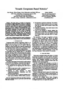
2.3.3 Genetic programming basics This part will cover the basic terminology of GP. First the primitives used in a GP, and the importance of choosing them carefully. Secondly, the use of fitness and how selection in executed will be discussed. Then it will cover the two most important operators in any evolutionary system: mutation and crossover. Finally, the rules of reproduction will be covered. Terminals and functions The terminals and functions are the two primitives with which any GP will build it’s structure. Both terminals and functions are referred to as nodes in the GP structure. The terminals and functions for any GP fill two different roles. The terminals will provide the system with values. This means that any constants, sensor values from sensors attached to a robot, or functions which takes no arguments constitute terminals. Using the tree analogy, any node which is a leaf is a terminal. Functions, on the other hand, are composed of any statements, operators, or functions available to the GP. Examples could be: boolean functions, arithmetic functions, conditional statements, loop statements, or subroutines. Using the tree analogy, any node which is a branch is a function (see figure: 2.1). When it comes to choosing the terminals and functions for any GP run, some care must be taken. It is important not to choose the function set to strictly. For example, using only AND will probably not solve any very interesting problems. But, on the other hand, it is important not to choose a set which is too large. Often a parsimonious approach, or the use of Occam’s razor, is recommended. The same carefulness is also importen in choosing the constants in any GP. The ability of the GP to combine chosen constants via arithmetic functions, will often compensate for a small number of constants. Fitness and selection For GP to work it must somehow choose which subset of the population is to undergo the genetic operators such as mutation, crossover, and reproduction. To do that GP utilises one of the most importen cornerstones in biologically evolutionary theory, namely fitness based selection. Where the best suited individual for a specific task (in biology often survival) will be allowed to reproduce.

CHAPTER 2. THEORY

16

+

Function/ Branch

−

10

5

5

Terminal/ Leaf

Figure 2.1: Overview of a GP tree structure

This theory which was first proposed by Charles Darwin [Dar28], inspired by the 1798 essay by Thomas R. Malthus, On the Principle of Population, where the Malthusian Crunch was introduced (see section 2.2.4). Two other well know theories deserves to be mentioned her: First, Wright’s theorem which states that natural selection increases the adaptation of individuals to their environment; and Fisher’s fundamental theorem of natural selection which states that evolution requires fitness variance, and the more variance, the faster the population evolves. See [Rou96] for a more through discussion of both theorems. Since GP, as natural evolution, utilises the variation in fitness and selects the most fit, some sort of fitness function must be provided. Fitness functions can be very different depending on the problem which is to be solved. A fitness function must be able to measure how well a given program is to predict the output from the programs input. Examples of factors used in fitness functions could include:

 The number of walls hit by a robot.  Time spent travelling in a straight line.  Area cover in exploration.  A combination of any above. Once the GP has assigned fitness to all of the tested individuals selection must be initiated. Selection can be viewed as the competition between individuals within the subset† of the population chosen for testing. Several standard selection mechanisms exists, including fitness-proportional, rank, tournament, sigma scaling, and elitism. Here the first three will briefly be described. Fitness-proportional selection is perhaps the most common, and has definitely been the primary choice for many since it’s introduction by Holland [Hol92]. An individuals † The

subset can of course include all individuals in the population

2.3. GENETIC PROGRAMMING

17

chance to form offspring in the next generation is given by equation 2.3; where the probability of a particular individual’s selection, is the fitness of the individual divided by the fitness of the whole population. pi 

fi ∑j fj

(2.3)

The fitness-proportional selection has been criticised for it’s tendency to fuel premature convergence. Premature convergence occurs early in an evolutionary run, when the fitness variance is high, and a limited number of individuals will multiply quickly, thereby preventing the GP from doing any more exploration. The fitness-proportional selection has also been criticised for attaching differential probabilities to the absolute fitness value. Rank selection is another often used mechanism. The fitness value assigned to a particular individual is a function of the rank within the population. For linear ranking, which is often used, the probability is a linear function of the rank (2.4). pi 




1 i 1 p  p p  N N 1

(2.4)

where pN is the probability of the worst individual being selected, and pN that of the best being selected, and (2.5) p  p  2

(2.5)

should hold if the population size is to stay constant. Last, but not least, is tournament selection. This mechanism separates itself from the rest by not using the whole population, but only a true subset. Some group of the population, the tournament size, is randomly selected, and a selective competition is initiated. The traits of the fitter individuals are then allowed to replace the less fit. Tournament selection has one major advantages over, for an example, fitness-proportional selection. It does not require any centralised comparison module. This allows more parallelising and a general speed up of a GP. Mutations Mutation in GP and other Darwinian based systems, serves two beneficial purposes: i) Mutation sets the stage for evolution. Without mutation, there can be no variation in genotypes, hence no basis for evolutionary change (The Hardy-Weinberg law and Fisher’s Theorem). ii) Mutation works as a rescue operator; given that the GP is stuck in one, of potentially several local maxima, mutation can push the population off the peak, and hopefully towards the global maximum. Mutation, on the other hand, can also have a negative effect. If, for instance, the mutation rate of a given system, natural or artificial, is to high, all the beneficial effects of mutation will drown in its destructive forces. Crossover The crossover operator is, by far, the most importen operator of the GP. Given a tree based GP the crossover operator works in the following manner:

CHAPTER 2. THEORY

18

1. Select two individuals, based on the selection mechanism. 2. Select a random subtree in each parent. 3. Swap the two subtrees or sequences of instructions. The crossover operator closely mimics the process of biological sexual reproduction. Based on this notion, the crossover operator has been used to claim that GP search is more efficient than methods based solely on mutation. Koza [Koz92] argued that a population in a GP system contains building blocks; a building block can be any tree or subtree which is present within a fraction of the population. This hypothesis follows the same line of argument as the Building block hypothesis from genetic algorithms [Hol92]. Given the building blocks and crossover the systems should be able to combine “good” building blocks to more fit individuals, and small building block should be able to combine into larger building blocks, hence, making the GP search more efficient than other methods. A more thorough discussion of the viability of this hypothesis it outside the scope of this work, and can be found in chapter 6 of [BNKF98]. Asexual reproduction Asexual reproduction is, by far, the easiest operator to handle. When an individual is selected, it is copied, and there are now two of the same individual in the population.

2.3.4 Summary Genetic programming is a method which has shown great promise in a lot of areas. However, it still possesses some problems or challenges. First of all, the choice of functions and terminals is a major issue. Secondly, the mutation rate of a system must be carefully chosen, since mutation can go both ways. Last, but not least, lack of speed has long been the major problem with GP.

Chapter 3

Related Work I can see as far as I do because I stand on the shoulders of giants – Issac Newton

3.1 Introduction This section will first cover some of the work done in the fields of GAs and ANNs, then it will describe the work done with GP and robotics, most notable the work by Nordin and Banzhaf.

3.2 Work with genetic algorithms 3.2.1 Introduction Within the last couple of years a new approach in BBR has evolved; this involves some form, of simulated evolution. What is to be evolved has been heavily debated. One approach which seems to be growing is the use of a GA to evolve an ANN. The research within the field of GAs and ANNs can be divided into three groups: i) Those who use simulation only. ii) Those who use on-board evolution only. iii) Those who use some kind of hybrid approach, i.e. simulation and on-board. Nolfi et. al. defends the approach with GAs and ANNs by stating the following reasons. [NFMM94] i) “Neural networks can easily exploit various forms of learning during a life-time”, and like the Baldwin effect [Bal96] in GA shows, the “learning process may help and speedup the evolutionary process” [HN87], [FM90], [FP96]. ii) Neural networks are notable for there resistance to noise which is highly present in robot interaction with the real world. iii) The common agreement today is that primitives manipulated by evolution should be on the lowest level possible, to avoid the possibility of undesirable choices made by a human programmer. To support this approach Nolfi et. al. conducts three experiments with a Khepera robot, unfortunately all of these experiments were only supposed to roughly evolve the same ability, all of which were some kind of exploration. The experiments were 19

20

CHAPTER 3. RELATED WORK

divided into: evolution of controller in simulation only, and then testing on the physical robot; evolution on-board; and a hybrid solution, where the first 300 generations were in simulation and the last 30 on-board. Furthermore they used fixed ANNs, a single layer feed forward net with eight input- and two output nodes. As Stone [Sto94], and Harvey [Har92] notes, there is always some degree of human meddling no matter how low a level we evolve from. The use of fixed nets is not a perfect fit with the point of the risk of undesirable choices made by a human programmer. They did, however, show that it is possible and feasible to utilise a GA in constructing controllers for autonomous robots. They also concluded that it is better to employ the physical robot in the process, not in an on-board situation only, but in a hybrid way. Several other examples of use of GAs and ANNs has been described. Here I will divide the examples into three groups: simulation only, on-board only, and hybrid.

3.2.2 Simulation Nolfi demonstrated the possibilities of evolving non trivial behaviour, specifically a garbage collection robot, based on the Khepera robot with a gripper attached [Nol96]. Here several basic behaviour were pre-generated, such as: leave-nest, get-food, avoidobstacles. Then an ANN was constructed consisting of a feed-forward net with 7 sensory nodes, 16 motor nodes, and no internal nodes. The controller was evolved in simulation and then downloaded on the real robot for testing. He was able to show that the best fit individual was able to clean the arena of garbage. Animals and robots needs to function in a dynamic environment, for this they need a palette of different types of behaviours. In an example given by Yamauchi and Beer [YB94] foraging for food requires the following behaviours while exploring the environment. It needs to react to any threats or obstacles, remember the way back to it’s nest, and the location of any food sources. This means that if the animal is to forage in a efficient way, it requires the capabilities of “reactive and sequential behavior, as well as the ability to learn from experience”. To show that it was possible to evolve these behaviours Yamauchi and Beer implemented a 8-node continuous-time recurrent neural network, where the network parameters were encoded as a vector of real numbers in the GA. They then set up the task of landmark recognition to test this. The ANN was evolved in simulation and then tested on the physical robot, which was a Nomad 200. After 15 generations, the network was capable to recognise the landmarks in simulation. It was then transfered to the robot where is was able to correctly classify the landmarks in 85 % of the test cases. Harvey et. al. advocates the use of GA to evolve dynamical neural networks in simulation [HHC93]. They do, however, take the ANNs a step further. They describe a continuous real-valued networks with unrestricted connections and time delays between units. For their implementation the use a network with a fixed number of inputand output nodes, and no specified number of hidden nodes. They also stress the importance of the simulator being kept as close to reality as possible. They put forth the following techniques to do this: i) The simulator should be calibrated with the robot hardware involved. ii) Empirical data should be the base of sensor simulation. iii) Noise must be taken into account. These points are also elaborated in [JHH95]. The last point which was stressed by Harvey et. al. was that every robot which is going to do any thing useful; must have vision. To defend these view they implemented a simulator where the ANN was evolved, which should develop

3.2. WORK WITH GENETIC ALGORITHMS

21

wandering behaviour in an office like environment. Within the 50 generations available to the simulator wandering behaviour was evolved. To sum up, it is clear that this approach is useful for developing controllers for robots. Several prerequisites most hold for this approach to be successful. Firstly, the simulator must be as close to the robots reality as possible, meaning, for an example, that simulated sensors should be sampled from the real robot, or that noise should be generated to compensate for uncertainties in the real world. Secondly, the tasks seems to have to be somewhat limited, for this approach to work; which perhaps, according to Harvey et. al., could be remedied by vision. Lastly, perhaps the solutions where network parameters have been pre-defined, should be extended to open-ended evolution; as argued in [Har92].

3.2.3 On-board As described above it is better to employ the physical robot in any work done with a simulator. This enhances the performance once the real world is tackled. The extreme approach is to run everything on the physical robot, i.e. the GA/ANN framework and the testing. This on-board approach ensures that any physical limitations, or noise, will be handled by the system. Some of this work has already been described (see section 3.2.1), by Nolfi et. al. [NFMM94]. More thorough investigations has been done by Floreano et. al. [FM96a], where they describe a pseudo on-board system which consists of a Khepera robot connected to a work station. The work station generated the simple ANNs which only had three neurons; one input, one hidden, and one output. All of which received synaptic connections from all eight infra red sensors, and the hidden node. These were all downloaded onto the Khepera where each node could change its strength according to one of four Hebbian rules: i) pure Hebbian. ii) post-synaptic. iii) pre-synaptic. iv) covariance. The task were to follow the walls around in circular environment with an obstacle in the middle. After around 50 generations the best fit individuals were able to keep a straight trajectory around the area, without hitting the obstacle. Similar results were achieved in [FM94] were a similar problem were solved by only evolving synaptic strength. The results in the later work were, however, better [FM96b]. Steels argues for four major point in the use of evolution for development of robot controllers [Ste94]: i) the use of a sub- or pre-symbolic level in evolution. ii) The use of a “level playing field” where modules can not exhibit each other. iii) The use of on-board (on-line) evolution. iv) open functionality, as in [Har92]. To test these statements he constructed the PDL robot architecture. This architecture consists of three basic units. i) Quantities, which can be external, like sensor values, or internal, like world states. ii) Processes, differential equations which are dynamical relations between quantities. iii) Behaviour units, a regularity within the interaction dynamics between the robot and it’s environment. Furthermore, this architecture is guided by these two principles. All behaviour systems are active at the same time, and the influence of the different behaviour systems are summed to select the appropriate behaviour; this is also known as Arbitration. Steels use two experiments, one where he was suppose to evolve the behaviour system which enables the robot to move forward and backward, and another where the ability to come to a hold was sought after. Both problems were easily solved within an acceptable time frame.

22

CHAPTER 3. RELATED WORK

3.2.4 Hybrid As it has become clear there are problems both with only using simulation or on-board. Several people has tried to improve the quality of robot controllers by using a hybrid method. One interesting work by Miglino et. al. addresses several of the problems both with simulation and on-line running [MLN95]. Their work was made on a Khepera robot. Where the weights of an ANN was evolved in simulation, and then tested on the real robot. One of the major problems with simulation is the lack of perfect hardware. When a robot has several sensors they should return the same value under the same circumstances; alas, no hardware does that. So the simulator used by Miglino et. al. was build on a sample of the real world, through the physical sensors on the Khepera. This approach greatly improved the simulator. Miglino et. al. also investigated the introduction of “noise” into the world model. This was based on the hypothesis that the world is dynamic, hence noisy. The introduction of noise also improved the performance of the robot, once it was tested in the real world. The noise issue has been investigated by many people, such as Jakobi [Jak97], Reynolds [Rey94b], and Jakobi et. al. [JHH95]. One thing which was observed by Miglino et. al., was that no matter how well they constructed their simulator a decrees in performance was often observed when the controller was introduced to the real environment. This problem was nicely solved by running the last few generations on the real robot. This work demonstrated that it can be feasible to run a simulation of a particular robot; as long as the problems of imperfect hardware, and the “noisiness” of the real world is addressed properly. The major benefit of simulation is the speed of the entire process. Simulation speeds up the otherwise tiresome process of running a full generational replacement on a real robot. Other work by Miglino and others also stresses the point of the simulation/embodiment solution. One work [MNT95], where wandering behaviour was evolved by an GA evolving the weight for an ANN; this time using a LegoT M robot. They used one population which ran in simulation only. One population where the evolutionary part was made on a workstation, and then tested on the real robot. As it could be expected the real-world population outperformed the simulated population, even though not by much. And the introduction of noise improved the simulated population. The conclusion in this work argued pretty much the same as in [MLN95], that the simulation/embodiment solution is feasible, and the solutions which is produced by this hybrid approach can perform acceptable. Quite a lot of work has been done with hybrid solutions, several of which has already been mentioned, others include Lewis and Fagg [LF92], Nolfi et. al. [NFMM94], Grefenstette and Schults [GS], Yamauchi and Beer [YB94], and Lund and Miglino [LM96].

3.3 Work with genetic programming 3.3.1 Introduction Historically most of the work done with adaptive BBR has been done with GAs and ANNs. More recently, with few exceptions, some work has begun to explore the pos-

3.3. WORK WITH GENETIC PROGRAMMING

23

sibilities of using GP as the evolutionary method.

3.3.2 Simulation Properly the first experiment with autonomous robots and genetic programming is the work of Koza and Rise [KR92], where they simulate a box pushing robot. The robot’s controller was evolved using a standard full generational replacement GP. The GP successfully found a solution in 45 generations. Craig W. Reynolds expanded the work by Koza and Rise. Both used high level functions, such as move-forward, turn-left, and turn-right [KR92]; turn, and look-forobstacle [Rey94a] (They both used arithmetic functions beside these high-level functions). The major difference between the work of Koza and Rise, and this is the use of a steady-state GP instead of full generational replacement. Steady-state is the opposite of full generational replacement, here only a sub-set of the population, instead of the whole population, is tested in each iteration. Even though, both of these experiments clearly shows that it is possible to evolve controllers using a GP, they also, [Rey94a] most prominent, show that robustness is quite another matter. The robustness of GP evolved controllers and a solutions to the problem is described in [Rey94b]. Reynolds repeated his experiments from [Rey94a], except that he added noise to the simulation; here noise is defined by taking the “worst of four noisy trails”, as in [HHC93]. As discussed in section 3.2.4, noise plays a very beneficial role in evolving robust controllers. This work by Reynolds shows that the simulation-noise connection also holds for GP. And that it is possible to evolve robust controllers using GP. Bennett expanded on the work by Koza and Rise. Inspired by parts of psychology, which argues that the mind works in a distributed way, and that there is no central unit which decides everything, he was interested in evolving a controller that could cope with several different problems at once: lawn mower, wall following, gold collector, and mine sweeper [III97]. The simulated world which this robot inhabits is made up of four squares – one for each problem – which are connected in the middle. The GP structure consisted of a “top tree” which, over time, contains sub trees for each problem. The evolutionary system worked on two levels: i) The meta-level, where the top tree was evolved, ii) The sub-level, where an ordinary evolution of the GP’s automatically defined functions (ADF) was evolved. With this work Bennett showed that a GP could discover good programs, which could solve different problems by organising the control program so that it could select the appropriate behaviour when needed. Even more advanced work has been done by Lee et. al., who presented some work where they used an evolutionary island model to evolve behaviour for a Khepera robot [LHL97] The controllers which were evolved were defined at the logic level. The controller works almost as a boolean network, where conditional structures are used to select appropriate motor commands and activating behaviour primitives. The GP system was used to evolve these boolean controllers. They evolved behaviour for box-pushing and box-side-following, each was controlled by a separate behaviour primitive. The GP consisted of three non-terminals: dummy root nodes, which was used to connect some arbitrary number of sub-trees,

CHAPTER 3. RELATED WORK

24

here a PROG† which allows several instructions to be executed in a sequence; logic components, which were AND, OR, NOR, XOR; and comparators, which were  . The terminals were sensor values and thresholds, all were between 0 and 1 inclusive. The controllers were evolved in simulation with sampling of the robots sensors, as described in [Nol96]. When a suitable controller was evolved, in 50 generations, it was transfered to the robot for testing. When the two primitives were evolved, box-pushing and box-side-following, a arbitrator was evolved to decide when the two primitives should be used. In line with the work of Bennett [III97], this work by Lee et. al. showed that it is possible and feasible for a GP to evolve the special structure of behaviour primitives, and to solve more complex problems than the typical wall-following and the like. Another work by Koza et. al. [KBKA97], investigated the use of GP for evolving controllers to navigate a robot safely to any arbitrary point in minimal time. This work is more or less an extension to the work of Bennett [III97], with the little twist, that they also use a GP to evolve an analog electrical circuit to use with their evolved controller in a robot. Other work done in this field includes [Han94].

3.3.3 On-Board Since GP tends to be very time consuming there hasn’t been much work done in real time on-board GP in robots. However, lately some work has emerged from Department of Computer Science, University of Dortmund led by Wolfgang Banzhaf and Peter Nordin [NB97b]. This part will cover this work, which is the base of the work in this thesis. Introduction Banzhaf et. al. has been working on a genetic program running on-board a Khepera robot. The work has been done in two major parts: i) evolving controllers for simple problems, e.g. obstacle avoidance and wall following [NB95]. ii) more advanced hierarchical structures, where they utilise the basic behaviour evolved in the first part [ONB96]. All of the experiments is conducted using a GP where the individuals consists of variable length strings of 32 bit instructions for a register machine. The GP individual is represented in a linear fashion, where each node is an instruction for the register machine. The 32 bit instructions represent basic arithmetic operations such as a  b  c or d  b  9. The actual format of the instructions is the machine code format of a SUN-4 (Sparc). The population is typically quite small, i.e. under 50 individual. The GP itself is a steady-state system using tournament selection with the size of 4, where candidate one and two returns one parent, and candidate three and four supplies the second parent. Both “losers” are deleted and the children from the crossover are added to the population instead of the two “losers”. The crossover is a two-point string crossover, where each node is the crossover unit. Crossover can occur on either side of the node, but because of the integrity of the program, never inside a program. Mutation flips bits within a 32-bit block, and makes sure that only legal functions, variables, or constants occurs [NB97a]. The design of this system are based of the following assumptions [BNO97] (paraphrased): †A

construction very familiar to any LISP programmer

3.3. WORK WITH GENETIC PROGRAMMING

25

 Any behaviour can be produce with a general purpose language.  GP produces symbolic output, in contrast to ANNs.  Goal definition is only done by deciding on a fitness function.  GP has a built-in tendency to generalise from presented situations.  This particular type of GP is fast, memory efficient, and can run on a robot with very limited computational power.

Another problem which is removed in this GP, is the need for the same starting point for all test cases. This is handled implicit by the way that each individual is tested against a real-time fitness case, thereby making a probabilistic sampling of the environment [NB95]. This approach could give rise to “unfairness” in testing individual, as some individual could have more “luck” with their starting point. But this problem is removed over time. The randomness in the starting point for each individual results in two types of survival strategies: i) cooperative strategy where the individual manages to fulfil the fitness criteria, even under poor conditions. ii) competitive strategy where the individual tries to minimise the fitness of the other individuals by placing the robot in situations which are very hard to get out of [BNO97]. The two training environments were: one small rectangular shaped world 30  40 cm., and one larger and irregular shaped rectangular world 70  90 cm., where object could be placed at arbitrary locations [NB97a]. Basic model In the basic model the interest was on evolving obstacle avoidance in a sense-think-act context. The GP systems evolved controllers in real time, using real noisy sensorial data [NB95]. This experiment was not compiled to run autonomously on the Khepera, it ran on a workstation were it communicated with the Khepera for sensory information, and for sending information to the motors. Hence, this experiment was not on-board but on-line. The small population, typically less that 50 individuals, of genetic programs each used six values from the sensors, and produced two output values for the motors. Each individual does this autonomously. The fitness function was divided into two parts; a pain and a pleasure part. The pain part was just the sum of all sensory input, and the pleasure part was assigned by measuring how log the robot ran straight and fast. See equation (3.1), where m1 and m2 are motor 1 and motor 2, and pi is the sum of the sensors. The goal is to minimise the function. f 

∑ pi  15

m1  15 m2  m1 m2 

(3.1)

The function set for the GP in this experiment was: addition, subtraction, multiplication, shift left, shift right, and, exclusive or, and or. The population size was 30, crossover probability was 90% and mutation probability was 5%. The system also had 256 nodes as maximum length of any given individual. This experiment showed that exploratory behaviour came right away. This was due to the diversity in the initial randomly generated programs. During the first minutes, the robot bumped in to the wall, but over time the bumping became less and less frequent.

CHAPTER 3. RELATED WORK

26

After about 20 minutes, which is approximately 100-150 generations, the robot had learned obstacle avoidance. In the more complex environment it took around a hour to evolve obstacle avoidance. The obstacle avoidance experiment was expanded to include object following [NB97b]. In this work the set up was almost identical to the first experiment. There was a few differences: i) To make sure that the algorithm was not brittle, it was evolved in the complex environment, and then tested in an even larger environment (100  100) cm. ii) In the object following experiment a new fitness function was used (see equation 3.2), where s1 to s4 is the four forward looking sensors. iii) The algorithm was crosscompiled and tested on-board; giving much the same result. f 




s1  s2  s3  24 1000 

2

(3.2)

For the object avoidance experiment the results were identical to the ones in [NB95]. It took around one hour to learn good object avoidance, and i 90% of the experiments the robot learned to reduce collisions to fewer than two per minute. The object tracking experiment the robot actual learned the appropriate behaviour faster than the case of object avoidance; it took around 30 minutes. The reason could most properly be the relative easier fitness function. The most interesting part of this work is the use of on-board evolution. Both tests were executed on-board with the same framework as the on-line version. Both performed identically. The only problem were that the battery time on a Khepera is approximately 40 to 60 minutes, which is very close to the minimum time required for training. Both papers showed that it is possible to evolve robust controllers for a robot using GP. The most interesting part is that it is also possible to evolve in total seclusion. ADF model As an extension to the work described in the last part, Banzhaf et. al. investigated the possibility of evolving high-level action selection based on the basic behaviour mentioned above [ONB96]. This work uses the on-board version of their GP. This GP consists of five populations, one for each action primitive and the control structure: go ahead Moving straight at maximum speed. avoid obstacle Avoid obstacle at maximum speed. seek obstacle The inverse of avoid obstacle. find dark Searches for darkness to move to. select action The populations of selection mechanisms. When the system is running it feeds data into the data registers of each action selection mechanism. Four are selected for tournament selection, they each select one of the four action primitives, through tournament selection. The winners replaces the losers and genetic operators are used. The performance of the system was tested in three different experiments: collision avoidance, wall following, and hiding in the dark. As an example, the robot showed effective collision avoidance after 800 cycles.

3.4. SUMMARY

27

After a period of four to seven minutes, the robot shows robust behaviour with it’s action primitives. This work was even further extended in [BNO97], where the action primitives and action selectors were evolved. Further more, a memory-based GP was introduced. This splits the GP into two separate processes. One which communicates with sensors and motors as well as storing events, 50 event vectors are recorded. The other process tries to learn an induce a model of the world. This memory addition speeds up the learning process with about a factor 40. Further more, an interesting thing which occurred was that a kind of “childhood” had to be introduced to make the system work in the best possible way. When using the standard memory model, a FIFO model, the robot forgot important early experience. The solution was to introduce a childhood, where the robot learns quickly, and the memories are hard to forget. The robot performed better if it became harder and harder to memorise events the older it got. To achieve a robust system with learning, the population had to be increased from 50 to 10.000 [NB97a]. This removes the possibility of a true autonomous robot, since only 256KB of memory is available on the Khepera. All in all, this work shows that primitive behaviour as more than possible to evolve using GP, both in an on-line and on-board fashion. Even more intelligent, or high level behaviours, can also be evolved by the same technique. Yet, the robot’s limited hardware removes the possibility of true autonomous running when learning is included; however, this is a practical problem, which can be solved cheap and easily.

3.3.4 Hybrid Since the use of on-board GP still is very limited, there is not much literature available beside the work done by Banzhaf et. al. Hence, not very much has been done on hybrid solutions either. Marc Ebner has done some work on the use of GP both in simulation and onboard [Ebn98]. He investigated if a GP could evolve a controller for a large mobile robot (a Real World Interface B21); Not only a program for avoiding walls, but also a hierarchical structure a´ la ADF. First an experiment in simulation of the world and the robot was conducted. Here several fitness cases were tested, and the most successful were then used on-board. the on-board evolution followed the same guidelines as the simulated. The experiment had a population size of 75, tournament selection with size 7 was used, the maximum time per fitness case were 300 s., and the whole system was run for 50 generations. The simulated solution and the on-board solution came out almost equal. Due to the time problem (evolution took 197 hours, the whole experiment 2 months) only one run was performed. The experiment still showed that it is possible to evolve a hierarchical control architecture with GP. Ebner also concluded that it should be feasible to use computer simulations, and especial to find the main parameters for the run on the real robot.

3.4 Summary This chapter has describe a lot of the work done with autonomous behaviour based robotics today. Most of this work includes some kind of evolutionary method; most often a genetic algorithm which evolves artificial neural networks. The technique has

28

CHAPTER 3. RELATED WORK

proven most successful when simulation is used, preferable in conjunction with online evaluation. This goes nicely hand in hand with Brooks [Bro91] situatedness and embodiment. ANNs and GAs in particular are sensitive to certain problems. According to Banzhaf et. al. [BNO97] GP can solve many of these problems. The major problem with GP has for a long time been the slowness of the system, but this problem has also been solved – it can even be faster than related evolutionary systems evolving ANNs ([NB97a] p. 17). All in all on-board, or at least on-line, GP seems to be a promising approach in behaviour based robotics.

Chapter 4

Approach Beware of bugs in the above code; I have only proved it correct, not tried it – Donald E. Knuth

4.1 Introduction This chapter will cover the work done with the robot, the design and the implementation of the GP. First an introduction to the Khepera robot will be presented; secondly, the design of the GP with details from the implementation will be covered.

4.2 The Khepera

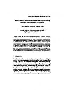
Figure 4.1: The Khepera robot

29

CHAPTER 4. APPROACH

30

The experiments in this work has been carried out on a standard autonomous mobile robot (see figure: 4.1), the Swiss made mobile robot platform Khepera [MFI93]. The Khepera has eight infrared proximity, or light intensity, sensors; all of which are distributed around the robot, in a circular pattern. The robot has a diameter of six cm. and a height of three cm. It is also equipped with two separately controllable motors; a MotorolaTM 68331 processor with 256k of memory; a ROM containing the operating system which has simple multitasking; and the possibility of connecting it to a workstation with a serial cable. There are two possible ways of controlling the robot. Either the algorithm could be run on a workstation, communicating with the robot through a serial line; or the algorithm could be complied for the MotorolaTM , and down-loaded to the robot, which then runs the entire program.

4.3 Genetic programming structure Here a short introduction to the framework will be given. Then individuals, initialisation, selection, crossover, and mutation will be covered more throughly. The structure chosen for this work is loosely based on a synthesis of the work done by Banzhaf et. al. (covered in section 3.3.3), and the work by Keith and Martin [KM94]. Evolutionary method

Reproduction

Crossover/mutation

Khepera Robot



 





  

 

Motor commands

Selection

Population X individuals

Sensor values

Selection method

Figure 4.2: Overview of the framework Since robots should behave in an autonomous fashion ([Bro91] [NB97b]). The system run entirely on the physical robot, as can be seen in figure 4.2 (Adopted from [BNO97]). The robot is connected to the workstation, solely for dumping statistical information and for receiving power. This setup contains a population of C programs, which are exposed to selection. All input from the world arrives through the eight infrared sensors on the Khepera. Outputs are written to the two motors, and values from both sensors and motors are used for selection (fitness calculation).

4.3. GENETIC PROGRAMMING STRUCTURE

31

Initialise robot

Initialise population

Select father

Select mother Main loop Crossover

Mutation

Figure 4.3: Systems execution cycle

The choice of ANSI C as the language is based on the work of Banzhaf et. al. They, however, used an assembler language for their evolutionary generated programs. I argue that even though the speed of the system properly will diminish when using a general purpose language, as opposed to assembler, the usability of evolved programs are higher with this setup. Not only will the code generated be portable, but it will be much more readable; and the long term goal here is not to make very efficient and commercial successful robots, but to understand what is going on. The overview of the GP made for this thesis is:

 Implemented in ANSI C.  The GP uses a steady state method, and tournament selection with two times two individuals for the tournament.

 The crossover is one point random for each parent.  The two winning parents are kept in the population.  Mutation is either changing one terminal for another, or changing one function.  Individuals are a pointer-based dynamic structure. i.e. no constrains on the length of the individual.

 Compiled on a Solaris workstation using GCC 2.8.1 cross-compiler for the Motorola TM 68k processor.

 The system is down-loaded and executed on-board the micro controller.

CHAPTER 4. APPROACH

32

The systems goes through two preliminary steps initialise robot and initialise population. It then goes through a loop consisting of selection, crossover, and mutation (see figure 4.3).

4.3.1 Individuals The population consists of a fixed number of individuals, typically 50 or less. Since the system should be as dynamic as possible, the individuals are represented as a pointer structure with no maximum length (see figure 4.4). This could potential lead to a population with very long individuals, and the size of these individuals could surpasses the memory available on the robot. But since a minimum- and maximum length is given when initialising the population, this hasn’t been a problem. individual length fitness mate number elem

element

element

next func term

element

.....

next func term

NULL function name arity expression

next func term

NULL

NULL

NULL

terminal

terminal

name value

name value

int gpmul (int listofargs[]){ return listofargs[0] * listofargs[1]; };

Figure 4.4: Overview of the individuals structure The individuals are represented in a linear fashion. This should not be mistaken for a linear GP. The GP used in this work is actual a tree-based GP, it is just represented in a linear structure, and all manipulation is done on the linear structure. This is, with some modifications, based on the work by Keith and Martin [KM94]. The use of a tree-based GP in a linear form is different from the work by Banzhaf et. al. where a true linear GP was used (see section 3.3.3). All individuals consists of two parts. i) Information about the individual. ii) The C program. Any individual has the following elements:

4.3. GENETIC PROGRAMMING STRUCTURE

33

 length A integer containing the length of the individual. fitness The integer value of the individuals fitness. mate Boolean value to keep track of whether or not this individual has been selected as a parent of child. number The number of the individual, used for debugging purpose. elem A pointer to the first node in the individual’s program. The elem is the first node in the pointer array containing the C program. All nodes has the following in common:

 next The pointer to the next node in the array. Last one point to NULL. func A pointer to a function. Contains NULL if the node is a terminal. term A pointer to a terminal. Contains NULL if the node is a function. Terminals and function has one thing in common; they both have names. These names are only for readability. A function contains the following variables:

 name The name of the function, e.g. *, -, +, /. arity The number of arguments handled by the function. expression A pointer to a function, of the form: int (int listofargs[]){ return ; }; The terminals are short structures, they only contain the name of the terminal, e.g. sensor0, constant1. They also contains the value of the particular terminal. The initialisation is done with two parameters minimum-length and maximum-length. To insure the integrity of the random generated programs the arity of the functions selected minus one was added to a checksum, and in case of terminals one was subtracted from the checksum. When the expression is build the checksum must be minus one to guaranty a legal expression. This can be done purely random, but to speed up the process a trick from [KM94] was used: if((openbranch + currentlength) >= indiv->length){ force terminal selection } Where openbranch is the sum of the selected functions arity, minus one for each terminal selected. So when the expression is filed with functions and the rest of the available node has to be used for terminals to ensure the integrity; terminals are selected.

4.3.2 Reproduction To have a reproduction system in evolutionary computation selection is necessary. And either crossover or mutation must be used, more often than not, both crossover and mutation is used, as is the case in this work.

CHAPTER 4. APPROACH

34 Selection

The selection used in this system is based on the probabilistic sampling of the environment introduced by Banzhaf and Nordin in [NB95]. Here each individual is tested on a new fitness case, i.e. a new place in the environment. A discussion of this method can be found in ([NB95], [NB97b]) and others. The selection itself is straight forward. It is tournament selection with the size of four within a steady-state GP. Two parents are selected based on their fitness returned by the fitness function, tested on-line in the real environment. For an example, if obstacle avoidance is sought the function (4.1) could be used. f  α





m1  m2   m1 m2   β 

7

∑ si

(4.1)

0

Where α and β are constants used for scaling, m1 and m2 are the values of motor one and two, and si are the sensors. The two individuals who “lost” the tournament selection would be deleted and used for the children returned from the crossover function. Crossover Parent 1

Parent 2

Child 1

Child 2

>

>

>

>