Hindawi Publishing Corporation Journal of Chaos Volume 2014, Article ID 659647, 13 pages http://dx.doi.org/10.1155/2014/659647
Research Article Adaptive Control for Modified Projective Synchronization-Based Approach for Estimating All Parameters of a Class of Uncertain Systems: Case of Modified Colpitts Oscillators Soup Tewa Kammogne and Hilaire Bertrand Fotsin Laboratory of Electronics and Signal Processing, Department of Physics, Faculty of Science, University of Dschang, BP 67, Dschang, Cameroon Correspondence should be addressed to Soup Tewa Kammogne;
[email protected] Received 14 October 2013; Revised 6 January 2014; Accepted 6 January 2014; Published 12 March 2014 Academic Editor: Ren´e Yamapi Copyright © 2014 S. T. Kammogne and H. B. Fotsin. This is an open access article distributed under the Creative Commons Attribution License, which permits unrestricted use, distribution, and reproduction in any medium, provided the original work is properly cited. A method of estimation of all parameters of a class of nonlinear uncertain dynamical systems is considered, based on the modified projective synchronization (MPS). The case of modified Colpitts oscillators is investigated. Through a suitable transformation of the dynamical system, sufficient conditions for achieving synchronization are derived based on Lyapunov stability theory. Global stability and asymptotic robust synchronization of the considered system are investigated. The proposed approach offers a systematic design procedure for robust adaptive synchronization of a large class of chaotic systems. The combined effect of both an additive white Gaussian noise (AWGN) and an artificial perturbation is numerically investigated. Results of numerical simulations confirm the effectiveness of the proposed control strategy.
1. Introduction Synchronization of chaotic systems and their potential applications in wide areas of physics and engineering sciences is currently a field of great interest ([1, 2] and references cited therein). The first idea of synchronizing two identical chaotic systems with different initial conditions is introduced by Pecora and Carroll [3] and the method is realized in electronic circuits. Synchronization techniques have been improved in recent years, and many different methods are applied theoretically and experimentally to synchronize the chaotic systems which include back stepping design technique [4], projective synchronization (PS) [5], modified projective synchronization (MPS) [6, 7], generalized synchronization [8], adaptive modified projective synchronization [9], lag synchronization [10], anticipating synchronization [11], phase synchronization [12], and their combinations [13]. Synchronization may involve several systems without a prescribed hierarchy (bidirectional) as it is the case in synchronization of networks of
systems [14, 15], often happening naturally, for instance, in certain biological systems. Another intensive area of research to emphasize within bidirectional synchronization is the study of the consensus paradigm (see an excellent text in [16]). Amongst all kinds of chaos synchronization, MPS is the state-of-the-art of synchronization schemes. MPS means that the master and slave systems could be synchronized up to a constant scaling matrix. Recently, various control methods which include adaptive control [17, 18] and active control [7, 19, 20] have been introduced. Most of the works done on MPS of chaotic systems have used active control method since it is easy to design a control input and to deal with equations including scaling functions. The controller based on the active control method is complex and contains various variables, so it may not be suitable for real practical purpose. In fact, it is obvious that practical controllers should have simple structures. Besides, the projective synchronization (PS) has been used in the research on secure communication
2 [21] because of the unpredictability of the scaling factor which may be a useful element. Adaptive control technique is used when the system parameters are unknown. In adaptive method, control law and a parameter update rule for unknown parameters are designed in such a way that the chaotic response system is controlled by the chaotic drive system. Most of the studies in synchronization involve two identical/nonidentical systems under the hypotheses that all the parameters of the master and slave systems are known a priori. A controller is constructed with the known parameters and systems are free from external perturbations. But in practical situations the uncertainties like parameter mismatch and external disturbances may destroy the synchronization and even break it. So it is necessary to design an adaptive controller and parameter update law for the control and synchronization of chaotic systems consisting of unknown parameters to get rid of internal and external noises. In the presence of model uncertainties and external disturbances, an appropriate adaptive control scheme is applied to stabilize a group of chaotic systems. In [22] Salarieh and Shahrokhi proposed an adaptive synchronization of two different chaotic systems with timevarying unknown parameters. An adaptive synchronization between two different hyperchaotic systems was developed by Wu et al. [23] while Li et al. developed a complete (anti) synchronization of chaotic systems with fully uncertain parameters by adaptive control [24]. In [25] Wang et al. present an adaptive control and synchronization for chaotic systems with parametric uncertainties. The same control strategy is used by Mossa et al. for the antisynchronization of two identical and different hyperchaotic systems with uncertain parameters [26]. From the literature survey, it is seen that, with the development of nonlinear control theory, nowadays adaptive projective synchronization method has become very much effective to control and synchronize the chaotic and hyperchaotic systems with uncertain parameters and external disturbances. Recently, many authors have studied the adaptive synchronization for the chaotic systems. In [27] Shen et al. demonstrated that two chaotic Colpitts circuits can be properly synchronized with employment of adaptive controllers while the circuit parameters and the channel are time varying. An adaptive projective synchronization between different chaotic systems with parametric uncertainties and external disturbances was presented by Mayank et al. [28] while Jia et al. develop a generalized projective synchronization of a class of chaotic (hyperchaotic) systems with uncertain parameters [29]. Most of the adaptive control scheme is based on the dynamic parameter estimation. In their book entitled Stable Adaptive Systems [30], Narendra and Annaswamy show that the estimation is feasible when the parameters of the chaotic system can be written in the matrix form. This approach was used in 1991 by Mossayebi et al. to present an adaptive estimation and synchronization of chaotic systems [31]. The authors enlarge the parameter estimation concept extended to well-known chaotic systems in the literature. Nowadays, many other works are carried out to show that this topic is not new in nonlinear science but there is not generalized
Journal of Chaos method planned for this issue. The problem of estimating the unknown parameters using adaptive control has been extensively investigated in the literature for linear and nonlinear systems. For instance, in [32], Fotsin and Daafouz analyzed the adaptive synchronization of uncertain chaotic Colpitts oscillators based on parameters identification. Based on Lyapunov stabilization theory, Huang et al. [33] proposed an adaptive controller with parameters identification for synchronizing a class of chaotic systems with unknown parameters. In the work [34], synchronization-based estimation of all parameters of chaotic systems from time series is presented by Huang. But we notice that the underlying assumption in those papers is that the chaotic systems used as benchmark examples to investigate synchronizations are in a form that provides an easy identification of these parameters. The techniques mentioned in the above articles are not suitable for direct estimation of all system parameters of the circuits in which certain coefficients are arguments of some other nonlinear functions (jerk family, modified Colpitts, etc.). An adequate estimation of the MCO parameters then appears inescapable because of its many advantages that it offers in the various chaos applications. To the best of our knowledge there is no study in the synchronization between two identical chaotic oscillators having the topology described above with estimation of all its parameters. Besides the topology of the modified Colpitts oscillator presents a complex nonlinear term in exponential form and one of our purposes consists in estimating its arguments. Recently, there have been many efforts for the study of dynamical properties of this oscillator introduced by Ababei and Marculescu in [35] where it was used in the qualitative numerical transmission of information. The particular feature of this oscillator is the real possibility to control chaos using a single resistor, without varying any parameter of the intrinsic Colpitts oscillator, which offers the possibility of an electronic analog or digital control on the system dynamics. Most previous studies in the literature have predominantly concentrated on standard systems such as the Lorentz, the classic Colpitts oscillator, the Chua system, the Chen system, the Lu system, or the R¨ossler system either in the studies of their stability analysis and periodic oscillations or of their synchronization. It has been shown that the MCO can exhibit complicated dynamics with reference to the classical Colpitts oscillator linked to its nonlinearity topology which is a great advantage in telecommunication. In general, the security of chaos-based communication systems is dependent on the complexity degree of master’s dynamics, carrying signal as well as the encryption scheme used [21]. There are few studies in the synchronization of the MCO [36, 37], though these systems are widely encountered in practice, in particular in communication [38]. In this paper, we first transform the original system equations of MCO by rigorous mathematical theory and secondly we will study modified synchronization of uncertain MCO which is presented based on Lyapunov stability theory. The organization of this paper is as follows. In Section 2 we first give a brief presentation of the model and its chaotic behavior is introduced. In Section 3, we present the theory of transformation of the MCO. Problem formulation is relaxed
Journal of Chaos
3
in Section 4. Main results presenting the synchronization behavior of two unknown MCO with artificial perturbation are studied in Section 5. Numerical simulations are given in Section 6. Finally, conclusions are presented in Section 7.
2. The Modified Colpitts Oscillator The simplest configuration of the MCO is shown in Figure 1(a) [36]. This circuit uses a bipolar junction transistor (BJT) as the gain element and a resonant network consisting of an inductor (𝐿) and a pair of capacitors (𝐶1 and 𝐶2 ). The resistor 𝑅𝑑 is the additive element compared to the classical system. The nonlinear element is the BJT (here the NPN type) for which the simplified model shown in Figure 1(b) consists of nonlinear voltage-controlled resistance 𝑅𝐸 and a linear current-controlled current source 𝐼𝐸 [39]. Parasite capacitances of the BJT can be neglected in the frequency range of oscillation since their effect would only be a frequency shift. We assume 𝛼𝐹 = 1, where 𝛼𝐹 is the common-base forward short-circuiting current gain. This corresponds to neglecting the base current. The V–I characteristic of the nonlinear resistor 𝑅𝐸 (which corresponds normally to the emitter-base diode) and its approximate expression are defined as usual by 𝐼𝐸 = 𝑓 (𝑉BE ) = 𝐼𝑆 [exp (
𝑒𝑉BE ) − 1] 𝑘𝐵 𝑇
𝑒𝑉 ≈ 𝐼𝑆 [exp ( BE )] , 𝑘𝐵 𝑇
(1)
where 𝐼𝑆 is the saturation current of the emitter-base diode, 𝑒 the elementary charge, 𝑘𝐵 the Boltzmann constant, and 𝑇 the absolute temperature. The thermal voltage at room temperature is given by 𝑉𝑇 = 𝐾𝐵 𝑇/𝑒 ≈ 26 mV. Here we set 𝐼𝑆 = 10−11 A. The base-emitter voltage drop 𝑉BE is given by 𝑉BE = −𝑢2 − 𝑅𝑑 (𝑖𝐿 + 𝑖𝐵 ) ,
(2)
where 𝑖𝐵 is the base current. Moreover, the relations between the currents are 𝑖𝐿 = 𝑖1 + 𝑖𝑐 ;
𝑖𝐿 = 𝑖2 + 𝑖3 − 𝑖𝐵 .
(3)
Since we have 𝑖𝐿 ≫ 𝑖𝐵 , the simplified state equations for the schematic in Figure 1(a) are the following: 𝑑𝑢1 𝑖𝐿 𝐼𝐸 = − , 𝑑𝑡 𝑐1 𝑐1
𝑢2 = 𝑉CC 𝑦,
𝑖𝐿 =
𝑑𝑦 = −𝑏0 − 𝑏0 𝑦 + 𝑧, 𝑑𝜏
(6)
𝑑𝑧 = 1 − 𝑥 − 𝑦 − 𝑐11 𝑧 𝑑𝜏 with 𝑏0 = 𝜃/𝑅𝑒 𝑐2 , 𝑏 = 𝜃𝐼𝑆 /𝑐2 𝑉CC , 𝑐11 = 𝜃(𝑅𝐶 + 𝑅𝑑 )/𝐿, 𝑎 = (𝑉CC /𝑉𝑇 ) (𝑅𝑑 /√𝐿/𝑐1 ), and 𝑎2 = 𝐼𝑆 𝜃/𝑐1 𝑉CC . Let us select the parameters: 𝐿 = 98.5 𝜇H, 𝑅𝐶 = 35 Ω, 𝑅𝐸 = 400 Ω, 𝑉CC = 𝑉EE = 5 V, 𝐶1 = 𝐶2 = 54 nF and 𝑅𝑑 = 0.5 Ω which yields 𝑎 = 2.25, 𝑏 = 192.3, 𝑏0 = 0.106𝑐11 = 0.934, and 𝑎2 = 8.51 ⋅ 10−11 ; the system shows a chaotic behavior characterized by a maximal Lyapunov exponent 𝜆 max = 0.06 which confirms the occurrence of chaotic oscillations.
3. Transformation Analysis of MCO Consider the dynamics system of MCO given by 𝑑𝑥1 = 𝑥3 − 𝑎1 exp (−𝑎𝑥3 − 𝑏𝑥2 ) , 𝑑𝜏 𝑑𝑥2 = −𝑏0 − 𝑏0 𝑥2 + 𝑥3 , 𝑑𝜏
(7)
𝑑𝑥3 = 1 − 𝑥1 − 𝑥2 − 𝑐11 𝑥3 . 𝑑𝜏 In order to quantify the parameters inside the exponential term argument, let us introduce the coordinates change in state and output-space: (𝑧1 , 𝑧2 , 𝑧3 ) = (𝑥1 , 𝑒−𝑏𝑥2 , 𝑒−𝑎𝑥3 ) .
(8)
Derivatives in the considered space are given by (𝑥1̇ , 𝑥2̇ , 𝑥3̇ ) = (𝑧̇1 , −
1 𝑧̇2 1 𝑧̇3 ,− ). 𝑏 𝑧2 𝑎 𝑧3
(9)
𝑧̇1 = −𝜎1 ln 𝑧3 − 𝜎2 𝑧2 𝑧3 , (4)
𝑢 𝑑𝑖𝐿 𝑉CC (𝑅𝐶 + 𝑅𝑑 ) 𝑢 = − 𝑖𝐿 − 1 − 2 . 𝑑𝑡 𝐿 𝐿 𝐿 𝐿 We now introduce a set of dimensionless state variables (𝑥, 𝑦, and 𝑧) where we normalize voltages currents and time according to the following relations: 𝜃 = √𝐿𝑐1 ,
𝑑𝑥 = 𝑧 − 𝑎2 exp (−𝑎𝑧 − 𝑏𝑦) , 𝑑𝜏
In these new coordinates, the system (7) takes the form
𝑉 𝑑𝑢2 𝑖𝐿 𝑢 = − 2 − CC , 𝑑𝑡 𝑐2 𝑅𝑒 𝑐2 𝑅𝑒 𝑐2
𝑢1 = 𝑉CC 𝑥,
Using (2), (3), and (5), the system of (4) can be rewritten in the following form:
𝑡 = 𝜃𝜏,
𝑉CC 𝑧. √𝐿/𝑐1
(5)
𝑧̇2 = 𝜎3 𝑧2 − 𝜎4 𝑧2 ln 𝑧2 + 𝜎6 𝑧2 ln 𝑧3 ,
(10)
𝑧̇3 = 𝜎0 (𝑧1 − 1) 𝑧3 − 𝜎7 𝑧3 ln 𝑧2 − 𝜎5 𝑧3 ln 𝑧3 . with 𝜎1 = 1/𝑎, 𝜎2 = 𝑎1 , 𝜎3 = 𝑏𝑏0 , 𝜎4 = 𝑏0 , 𝜎5 = 𝑐11 , 𝜎0 = 𝑎, 𝜎6 = 𝑏𝑎−1 , and 𝜎7 = 𝜎6−1 . The system (10) presents five parameters as system (7) which confirms the linearity of the transformation. 3.1. Dissipation and Existence of Attractors. Preliminary insights concerning the existence of attractive sets [40] that might coexist in the system could be gained by evaluating the volume contraction/expansion rate (Γ = 𝑉−1 𝑑𝑉/𝑑𝜏) of
4
Journal of Chaos
iL RC
VCC
L i1 ic iB
E Rd
IE
IC
VBE
u1
c1
𝛼E IE
C
i2
i3 Re
c2 u2
VEE IB ≅ 0 B
(a)
(b)
Figure 1: Circuit model: (a) Schematic of the Colpitts oscillator. (b) BJT model in common base configuration.
the oscillator modeled by (10) at any given point (𝑧1 , 𝑧2 , 𝑧3 )𝑇 of the space. The following expression can be derived: Γ=
𝜕𝑧̇1 𝜕𝑧̇2 𝜕𝑧̇3 + + 𝜕𝑧1 𝜕𝑧2 𝜕𝑧3 𝜎 +𝜎7 𝜎5 −𝜎6 𝑧3 )
= 𝜎3 − 𝜎4 − 𝜎5 − 𝜎0 + 𝜎0 𝑧1 − ln (𝑧2 4 𝜎 +𝜎
= 𝜎0 𝑧1 − ln (
(11)
𝛽0 𝜆3 + (𝑏0 + 𝑐11 ) 𝜆2 + (1 + 𝑏0 𝑐11 + 𝑚2 ) 𝜆 + 𝑚1 + 𝑏0 𝑚2 = 0, (13b)
𝜎
𝑧2 4 7 𝑧3 5 ), 𝜎 𝛿𝑧3 6
where ln 𝛿 = 𝜎3 − 𝜎4 − 𝜎5 − 𝜎0 and 𝑧̇ = (𝑧̇1 , 𝑧̇2 , 𝑧̇3 ). Consider the fact that the system (10) is dissipative which is expressed as follows: 𝜎 +𝜎
div (𝑧)̇ = 𝜎0 𝑧1 − ln (
𝜎
𝑧2 4 7 𝑧3 5 ) < 0. 𝜎 𝛿𝑧3 6
(12)
This condition implies that the solutions of the new system are bounded as 𝜏 → ∞. We may rewrite condition (12) as follows: 𝜎 +𝜎
𝑧1
0, 𝛽2 > 0, and 𝛽1 𝛽2 < 𝛽3 . According to Routh-Hurwitz criteria the equilibrium point is unstable. The singularity is saddle point. The transformation (8) leads to the following equilibrium point in the new space: (𝑧10 , 𝑧20 , 𝑧30 ) = (𝑥10 , 𝑒−𝑏𝑥20 , 𝑒−𝑎𝑥30 ) .
(13c)
̇ 10 , 𝑧20 , 𝑧30 )) = Then 𝐸 = (1.02; 4046.67; 0.48) and div(𝑧(𝑧 2.72 > 0 which confirms the divergence of trajectories at the equilibrium point. In fact, an infinitesimal deviation of the initial conditions will eventually result in the divergence of nearby starting orbits. After a while, the system initially unstable becomes dissipative and stays unchanged with respect to its dynamical variables which strongly justify the synchronization process of MCO in the space considered.
Journal of Chaos
5
1.5
0.6
0.6
0.4
0.4
1 0.2
y
x
z
0.2
0.5 0
0 0
0
100
−0.2
200
0
100
Time 𝜏
−0.2
200
0
100 Time 𝜏
Time 𝜏
200
(a) 0.6
0.6
0.6
0.4
0.4
0.4
0.2
z
y
0 −0.2
0.2
0.2
y
0
0
0
0.5
1
−0.2
1.5
0
0.5
x
1
1.5
−0.2 -0.5
0
x
0.5
1
z
(b)
Figure 2: (a) Time histories of MCO, (b) Phase portraits (versus 𝑥, 𝑦 versus 𝑥, 𝑦 versus 𝑧). 0.22
0.8
0.2
0.6
0.18
0.4
0.16
z3
z1
1
0.2 0
0.14 0.12
−0.2
0.1
−0.4
0.08
5
10
15
20
25
30
35
40
45
50
55
60
𝜏
(a)
5
10
15
20
25
30 𝜏
35
40
45
50
55
60
(b)
Figure 3: Time histories of MCO when no control is applied ((a) 𝑍1 versus time z, (b) 𝑍3 versus time).
3.2. Model Description. Let us consider a general class of chaotic systems described by the following differential equation: 𝑧̇ = 𝜙̃ (𝑧 (𝜏) , 𝜏) 𝜃1 + 𝜀̃ (𝑧 (𝜏) , 𝜏) 𝜃2 𝑝
+ ∑𝜃̂𝑖 Ω𝑖 𝜀 (𝑧 (𝜏) , 𝜏) ,
𝑝 = 3,
(14)
𝑖=1
where 𝑧 ∈ 𝑅 denotes the state vectors, 𝜙̃ : 𝑅𝑛 → 𝑅𝑛 are continuous function matrices, and 𝜀̃, 𝜀 : 𝑅𝑛 → 𝑅𝑛 are a continuous nonlinear function, where 𝜀̃ denotes the product part of the state variables and 𝜀 the made up function in 𝑛
which the arguments are the system variables and 𝜃1 , 𝜃2 , and 𝜃̂𝑖 are parameters vectors such that 𝜃1 , 𝜃2 , 𝜃̂𝑖 ∈ 𝑅𝑛̃×̃𝑛 and Ω𝑖 ∈ 𝑅𝑛×𝑛 , respectively. Note that many chaotic and hyperchaotic systems such as jerk family system, two-cell quantum-CNN, and modified Bloch equations with feedback field could be described by system (14). Expression (14) is an interesting form because it describes the whole complex chaotic system and makes its dynamics behavior analysis easy such as stability and bifurcations. Assumption 1. The states of the chaotic system described by (14) are bounded, and the nonlinear function with two
6
Journal of Chaos Proposition 2. If the master system (17) and slave system (18) asymptotically synchronize, then the systems (19) and (20) which were derived from the change of space also asymptotically synchronize, such that lim𝑡 → ∞ ‖𝑒(𝑡)‖ = 0 ⇒ lim𝑡 → ∞ ‖𝑒 (𝑡)‖ = 0, where 𝑒(𝑡) = 𝑦(𝑡) − 𝑥(𝑡) and 𝑒 (𝑡) = 𝑧̂(𝑡) − 𝑧(𝑡).
div(dz/d𝜏)
10
5 0 −5
0
2
4
6
8
10
Proof. Let us write 𝑓(𝑧(𝑡), 𝑡) as the sum of two functions: 𝑓 (𝑧 (𝑡) , 𝑡) = 𝜙 (𝑧 (𝑡) , 𝑡) + 𝜀 (𝑧 (𝑡) , 𝑡) ,
𝜏
z1
Figure 4: Divergence of the flow of MCO in the new space. 0.8 0.6 0.4 0.2 0 −0.2 −0.4 −0.6 0.08
(21)
where 𝜙(𝑧(𝑡), 𝑡) is the linear part of 𝑓(𝑧(𝑡), 𝑡) and can take the form: 𝜙 (𝑧 (𝑡) , 𝑡) = 𝐴𝑧 (𝑡) = 𝐴𝜓 (𝑥 (𝑡)) ,
(22)
where 𝐴 is a full rank constant matrix and all eigenvalues of 𝐴 have negative real parts. The simplest configuration of matrix 𝐴 is described by 𝐴 = diag(𝜆 1 , 𝜆 2 , . . . , 𝜆 𝑛 ). Synchronization error between system (19) and system (20) is defined as 0.1
0.12
0.14
0.16
0.18
0.2
0.22
0.24
𝑒 (𝑡) = 𝑧̂ (𝑡) − 𝑧 (𝑡) = 𝐴𝜓 (𝑦 (𝑡) , 𝑡) − 𝐴𝜓 (𝑥 (𝑡) , 𝑡) + 𝜀 (̂𝑧 (𝑡)) − 𝜀 (𝑧 (𝑡))
z3
Figure 5: Phase portrait of MCO in the new space in the presence of artificial pertubation.
= 𝐴 (𝜓 (𝑦 (𝑡) , 𝑡) − 𝜓 (𝑥 (𝑡) , 𝑡)) + 𝜀 (̂𝑧 (𝑡)) − 𝜀 (𝑧 (𝑡))
variables 𝑓(𝑎 V3 , 𝑏 V2 ) is locally Lipschitz; that is, there exists a positive constant 𝑘𝑓 such that
= 𝐴𝑀 ‖𝑒 (𝑡)‖ + 𝑀𝑀 ‖𝑒 (𝑡)‖
𝑓 (𝑎 V3 , 𝑏 V2 ) − 𝑓 (𝑎 ̃V3 , 𝑏 ̃V2 ) ≤ 𝑎 𝑘𝑓 ̃V3 − V3 + 𝑏 𝑘𝑓 ̃V2 − V2 , where V = (V1 , V3 , V2 ), 𝑎 and 𝑏 are positive constants. The relation (15) can be put in the following form: 𝑓 (𝑎 V3 , 𝑏 V2 ) − 𝑓 (𝑎 ̃V3 , 𝑏 ̃V2 ) ≤ 𝑀 (𝑎 , 𝑏 ) 𝑒⊥ ,
(15)
≤ 𝐴𝑀 𝑦 (𝑡) − 𝑥 (𝑡) + 𝑀 𝜓 (𝑦 (𝑡) , 𝑡) − 𝜓 (𝑥 (𝑡) , 𝑡) = (𝐴 + 𝑀) 𝑀 ‖𝑒 (𝑡)‖ = 𝑀∗ 𝑒⊥ (23)
(16)
with 𝑒⊥ = 𝑀 ‖𝑒(𝑡)‖ and 𝑀∗ = (𝐴 + 𝑀)𝑀 being chosen such that all eigenvalues of the matrix 𝑀∗ have negative real parts; the dynamic errors are asymptotically stable. This completes the proof.
where 𝑒⊥ = (‖̃V1 − V1 ‖, ‖̃V2 − V2 ‖, ‖̃V3 − V3 ‖)𝑇 , 𝑀(𝑎 , 𝑏 ) = 0 0 0 0 0 0 𝜀
[ 0 𝜀
] with 𝜀 = 𝑏 𝑘𝑓 and 𝜀 = 𝑎 𝑘𝑓 .
4. Problem Formulation
Let us consider two 3-dimensional chaotic systems which can be represented in a more generic form as follows: 𝑥̇ = 𝑓 (𝑥 (𝑡) , 𝑡) ,
(17)
𝑦̇ = 𝑓 (𝑦 (𝑡) , 𝑡) ,
(18)
where 𝑥 ∈ 𝑅3 and 𝑦 ∈ 𝑅3 are 3-dimensional state vectors of the system and 𝑓 : 𝑅3 → 𝑅3 is analytic. We assume that the asymptotic convergence of (17) and (18) is satisfied. In the new space, the coordinates can be written in the following form: 𝑧̇ = 𝑓 (𝑧 (𝑡) , 𝑡) ,
(19)
𝑧̂̇ = 𝑓 (̂𝑧 (𝑡) , 𝑡) ,
(20)
𝑧(𝑡) = 𝜓(𝑥(𝑡)), and 𝑧̂(𝑡) = 𝜓(𝑦(𝑡)) where 𝜓(∗) is a transformation function.
An illustration of the modified projective synchronization is now presented. Taking into account the synchronization between two chaotic systems, take the drive system as follows: 𝑧̇𝑚 = 𝜙̃ (𝑧𝑚 , 𝜏) 𝜃1 + 𝜀̃ (𝑧𝑚 , 𝜏) 𝜃2 𝑝
+ ∑𝜃̂𝑖 Ω𝑖 𝜀 (𝑧𝑚 , 𝜏) + 𝜉 (𝑧𝑚 , 𝜏) ,
𝑝 = 3.
(24)
𝑖=1
The response system is 𝑠 ̇ = 𝜙̃ (𝑠, 𝜏) 𝜃1𝑟 + 𝜀̃ (𝑠, 𝜏) 𝜃2𝑟 𝑚
+ ∑𝜃̂𝑖𝑟 Ω𝑖𝑟 𝜀 (𝑠, 𝜏) + 𝑢 (𝑧𝑚 , 𝑠, 𝜏) + 𝑢 (𝑧𝑚 , 𝑠, 𝜏) ,
(25)
𝑖=1
where 𝑠 = [𝑠1 , 𝑠2 , . . . , 𝑠𝑘 ]𝑇 ∈ 𝑅𝑘 , (𝑢; 𝑢 ) ∈ 𝐶ℓ [𝑅+ × 𝑅𝑛 × 𝑅𝑘 , 𝑅𝑘 , 𝑅𝑛 ] and ℓ ≥ 1, 𝜉(𝑧𝑚 , 𝜏) is the external disturbances
Journal of Chaos
7 ×10⁻¹⁰ 1
5
0.8
4 a1 (𝜏)
a(𝜏)
3 2 1 0
0.6 0.4 0.2
0
2
4
6
8
0
10
2
0
4
𝜏
8
6
8
10
(b)
0.4
200
0.3
150 b(𝜏)
b0 (𝜏)
(a)
0.2
100 50
0.1 0
6 𝜏
0 0
2
4
6
8
10
0
2
4
10
𝜏
𝜏
(c)
(d)
1 C11 (𝜏)
0.8 0.6 0.4 0.2 0
0
2
4
6
8
10
𝜏
(e)
Figure 6: Estimated values for unknown parameters. 0.5
g(𝜏)
0.45 0.4 0.35 0.3
0
2
4
6
8
10
𝜏
Remark 3. Chaos synchronization schemes such as complete synchronization and antisynchronization are special cases of modified projective synchronization when 𝛼 = 1 and 𝛼 = −1, respectively. From the definition of error signal (26), the error dynamics is 𝑒 ̇ (𝜏) = 𝛼𝜙̃ (𝑠, 𝜏) 𝜃1𝑟 + 𝛼̃𝜀 (𝑠, 𝜏) 𝜃2𝑟 𝑝
+ 𝛼∑𝜃̂𝑖𝑟 Ω𝑖𝑟 𝜀 (𝑠, 𝜏) + 𝛼𝑢 (𝑧𝑚 , 𝑠, 𝜏)
Figure 7: Time evolution of adaptive gain.
𝑖=1
bounded in magnitude ‖𝜉(𝑧𝑚 , 𝜏)‖ ≤ 𝜌 , 𝑢(𝑧𝑚 , 𝑠, 𝜏) is the controller attached in the response system to be determined later, and 𝑢 (𝑧𝑚 , 𝑠, 𝜏) is the adaptive controller used for synchronizing the reference model with perturbation. If there exists a function
∀𝑧𝑚 (𝜏0 ) , 𝑠 (𝜏0 ) ∈ 𝑅𝑛 , (26)
(27)
𝑚
+ 𝛼𝑢 (𝑧𝑚 , 𝑠, 𝜏) − ∑𝜃̂𝑖 Ω𝑖 𝜀 (𝑧𝑚 , 𝜏) − 𝜉 (𝑧𝑚 , 𝜏) . 𝑖=1
Let us choose the controllers in the following form: 𝑢=
𝛼 = diag (𝛼1 , 𝛼2 , . . . , 𝛼𝑛 ) satisfying lim ‖𝑒 (𝜏)‖ 𝜏→∞ = lim 𝛼𝑠 (𝜏) − 𝑧𝑚 (𝜏) = 0 𝜏→∞
− 𝜙̃ (𝑧𝑚 , 𝜏) 𝜃1 − 𝜀̃ (𝑧𝑚 , 𝜏) 𝜃2
1 ̃ (𝜙 (𝑧𝑚 , 𝜏) 𝜃1𝑟 − 𝛼𝜙̃ (𝑠, 𝜏) 𝜃1𝑟 − 𝛼̃𝜀 (𝑠, 𝜏) 𝜃2𝑟 𝛼 𝑝
+ 𝜀̃ (𝑧𝑚 , 𝜏) − 𝛼∑𝜃̂𝑖𝑟 Ω𝑖𝑟 𝜀 (𝑠, 𝜏) 𝑖=1
𝑝
then the systems (24) and (25) achieve modified projective synchronization, where 𝑒 = (𝑒1 , 𝑒2 , . . . , 𝑒𝑛 )𝑇 and we call 𝛼 a “scaling factor.”
+∑𝜃̂𝑖𝑟 Ω𝑖𝑟 𝜀 (𝑧𝑚 , 𝜏)) − Λ𝑒, 𝑖=1
(28)
8
Journal of Chaos
0 e2 (𝜏)
e1 (𝜏)
0.5
−0.5 −1
0
2
4
6
8
10
14 12 10 8 6 4
×10−9
0
2
4
6
8
10
𝜏
𝜏
(a)
(b) 0.01
e3 (𝜏)
0.005 0 −0.005 −0.01
0
2
4
6
8
10
𝜏
(c)
Figure 8: Synchronization errors: (a) 𝑒1 (𝜏), (b) 𝑒2 (𝜏), (c) 𝑒3 (𝜏).
where 𝜃̃1𝑟 = 𝜃1𝑟 −𝜃1 , 𝜃̃2𝑟 = 𝜃2𝑟 −𝜃2 , 𝜃̂𝑖𝑟 = 𝜃𝑖𝑟 −𝜃𝑖 , Ω𝑒𝑖 = Ω𝑖𝑟 −Ω𝑖 , and Υ𝑗 = diag(Υ1𝑗 , Υ2𝑗 , . . . , Υ𝑝𝑗 ), 𝑗 = (𝛼, 𝛽, 𝜆), are constant positive matrices.
1
eq
0.8 0.6
Theorem 4 (Barbalat’s lemma [41]). Let one consider an uniform continuous function 𝜋 : [0, ∞) → 𝑅 such that ∀𝜏 ∈ [0, ∞):
0.4 0.2 0
𝜏
0
2
4
6
8
10
𝜏
Figure 9: Time evolution of the dynamic error.
where Λ = diag(Λ 1 , Λ 2 , . . . , Λ 𝑛 ), Λ 𝑖 > 0 (𝑖 = 1, 2, . . . , 𝑛) are constants. One advantage of this type of controller is that it can be easily constructed through time-varying resistors, capacitors, or operational amplifier and their combinations, or using a digital signal processor together with the appropriate converters. Consequently, we get 𝑒 ̇ (𝜏) = (𝜙̃ (𝑧𝑚 , 𝜏) − 𝛼𝜙̃ (𝑠, 𝜏)) (𝜃1𝑟 − 𝜃1 ) + (𝛼̃𝜀 (𝑠, 𝜏) − 𝜀̃ (𝑧𝑚 , 𝜏)) (𝜃2𝑟 − 𝜃2 ) 𝑝
+ ∑ (𝜃̂𝑖𝑟 − 𝜃̂𝑖 ) Ω𝑒𝑖 (𝛼𝜀 (𝑠, 𝜏) − 𝜀 (𝑧𝑚 , 𝜏))
(29)
𝑖=1
lim ∫ 𝜋 (𝑡) 𝑑𝑡 𝑒𝑥𝑖𝑠𝑡𝑠 𝑎𝑛𝑑 𝑖𝑠 𝑓𝑖𝑛𝑖𝑡𝑒; 𝑡ℎ𝑒𝑛 lim 𝜋 (𝜏) = 0.
𝜏→∞ 0
𝜏→∞
(30b)
Theorem 5. For the given scaling factor 𝛼, the modified projective synchronization between drive system (24) and response system (25) will occur under the control law (28) and the parameter update rule (30b). Proof. Construct dynamical Lyapunov function as follows: 𝑝
1 2 𝑇̃ 1 1 𝜃V𝑟 + ∑𝜃̂𝑖𝑟𝑇 𝜃̂𝑖𝑟 . 𝑉̇ = 𝑒𝑇 𝑒 + ∑ 𝜃̃V𝑟 2 2 V=1 2 𝑖=1
Then the time derivative of Lyapunov function 𝑉 along the trajectory of error system (29) is 2
𝑝
V=1
𝑖=1
̇ 𝑇 ̃̇ 𝜃V𝑟 + ∑𝜃̂𝑖𝑟𝑇 𝜃̂𝑖𝑟 𝑉̇ = 𝑒𝑇 𝑒 ̇ + ∑ 𝜃̃V𝑟
− Λ𝑒 − 𝜉 (𝑧𝑚 , 𝜏) . The parameter update rule is
= 𝑒𝑇 (𝜙̃ (𝑧𝑚 , 𝜏) − 𝛼𝜙̃ (𝑠, 𝜏)) (𝜃1𝑟 − 𝜃1 )
𝑇
̇ = −(𝜙̃ (𝑧 , 𝜏) − 𝛼𝜙̃ (𝑠, 𝜏)) 𝑒 − Υ 𝜃̃ , 𝜃1𝑟 𝑚 𝛼 1𝑟 ̇ = −(𝛼̃𝜀 (𝑠, 𝜏) − 𝜀̃ (𝑧 , 𝜏))𝑇 𝑒 − Υ 𝜃̃ , 𝜃2𝑟 𝑚 𝛽 2𝑟 𝑇 ̇̂ 𝜃𝑖𝑟 = −(𝛼𝜀 (𝑠, 𝜏) − 𝜀 (𝑧𝑚 , 𝜏)) Ω𝑒𝑖 − Υ𝜆 𝜃̂𝑖𝑟 ,
(30a)
(31)
+ 𝑒𝑇 (𝛼̃𝜀 (𝑠, 𝜏) − 𝜀̃ (𝑧𝑚 , 𝜏)) (𝜃2𝑟 − 𝜃2 ) 𝑚
− 𝑒𝑇 ∑ (𝜃̂𝑖𝑟 − 𝜃̂𝑖 ) Ω𝑒𝑖 (𝛼𝜀 (𝑠, 𝜏) − 𝜀 (𝑧𝑚 , 𝜏)) 𝑖=1
Journal of Chaos
9 𝑇
ln 𝑧1 𝜀 (𝑧 (𝜏) , 𝜏) = [ln 𝑧2 ] , [ln 𝑧3 ]
𝑇 ̃ − 𝑒𝑇 Λ𝑒 − 𝜃̃1𝑟 (𝜙 (𝑧𝑚 , 𝜏) − 𝛼𝜙̃ (𝑠, 𝜏)) 𝑒 𝑇 𝑇 𝑇 Υ𝛼 𝜃̃1𝑟 − 𝜃̃2𝑟 (𝛼̃𝜀 (𝑠, 𝜏) − 𝜀̃ (𝑧𝑚 , 𝜏)) 𝑒 − 𝜃̃1𝑟 𝑝
𝑇
𝑇 Υ𝛽 𝜃̃2𝑟 − ∑𝜃̂𝑖𝑟𝑇 Ω𝑒𝑖 (𝛼𝜀 (𝑠, 𝜏) − 𝜀 (𝑧𝑚 , 𝜏)) − 𝜃̃2𝑟 𝑖=1
𝑝
− ∑𝜃̂𝑖𝑟𝑇 Υ𝜆 𝜃̂𝑖𝑟 − 𝑒𝑇 𝜉 (𝑧𝑚 , 𝜏) 𝑖=1
𝑇 𝑇 = −𝑒𝑇 Λ𝑒 − 𝜃̃1𝑟 Υ𝛼 𝜃̃1𝑟 − 𝜃̃2𝑟 Υ𝛽 𝜃̃2𝑟 𝑝
𝑖=1
(32) Since the systems (24) and (25) are contained in an attractor, we can suppose that the whole error system (27) can be in the domain Ω = {𝑒 ∈ 𝑅𝑛 , ‖𝑒‖ ≤ 𝑟0 , 𝑟0 > 0}. Set ‖𝜉(𝑧𝑚 , 𝜏)‖ ≤ 𝜌 and consider a bounded positive function Λ (𝜏) such that 𝜉(𝑧𝑚 , 𝜏) = −Λ (𝜏)𝑒. It is obvious to note that ‖Λ (𝑡)𝑒‖ ≤ 𝑟0 𝜌 . Then, (32) may be written as follows:
𝑝
𝑇 𝑇 Υ𝛼 𝜃̃1𝑟 − 𝜃̃2𝑟 Υ𝛽 𝜃̃2𝑟 ≤ −𝑒 (Λ − Λ (𝜏)) 𝑒 − 𝜃̃1𝑟
(33)
− ∑𝜃̂𝑖𝑟𝑇 Υ𝜆 𝜃̂𝑖𝑟 < 0.
For the sake of clarity and the matter to handle easily the calculations, expression (34) can be put in the particular form which will enable us to underline modified projective synchronization. Let us consider the following MCO master with artificial perturbation and slave systems: 𝑧̇1 (𝜏) = −𝜎1 ln 𝑧3 (𝜏) − 𝜎2 𝑧2 (𝜏) 𝑧3 (𝜏) − 𝑘𝑧1 (𝜏) , 𝑧̇2 (𝜏) = 𝜎3 𝑧2 (𝜏) − 𝜎4 𝑧2 (𝜏) ln 𝑧2 (𝜏) + 𝜎6 𝑧2 (𝜏) ln 𝑧3 (𝜏) ,
(35)
𝑧̇3 (𝜏) = 𝜎0 (𝑧1 (𝜏) − 1) 𝑧3 (𝜏) − 𝜎7 𝑧3 (𝜏) ln 𝑧2 (𝜏)
+ 𝜎6 𝑠2 (𝑡) ln 𝑠3 (𝜏) + 𝑢2 + 𝑢2 ,
(36)
𝑠3̇ (𝜏) = 𝜎0 (𝑠1 (𝜏) − 1) 𝑠3 (𝜏) − 𝜎7 𝑠3 (𝜏) ln 𝑠2 (𝜏) − 𝜎5 𝑠3 (𝜏) ln 𝑠3 (𝜏) + 𝑢3 + 𝑢3 ,
𝑖=1
We can see that 𝑉 is positive definite if Λ − Λ (𝜏) ≤ 0 and 𝑉̇ is negative definite; according to Lyapunov stability theory, the error vectors 𝑒𝜎 (𝜎 = 1, 2, . . . , 𝑛) asymptotically tend to zero, leading to the modified projective synchronization between drive (24) and response system (25). Therefore, the proof is completed.
5. Main Results The equations of MCO in the new space can be expressed as in equations (24), with the following parameters:
0 0 0 Ω2 = [0 0 𝑧2 ] , [0 −𝑧3 0 ]
0 𝜃̂2 = [𝜎6 ] . [𝜎5 ]
𝑠2̇ (𝜏) = 𝜎3 𝑠2 (𝜏) − 𝜎4 𝑠2 (𝜏) ln 𝑠2 (𝜏)
𝑝
𝑧1 𝑧𝑚 = [𝑧2 ] , [𝑧3 ]
𝜎1 𝜃̂1 = [𝜎4 ] , [𝜎7 ]
𝑠1̇ (𝜏) = −𝜎1 ln 𝑠3 (𝜏) − 𝜎2 𝑠2 (𝜏) 𝑠3 (𝜏) + 𝑢1 + 𝑢1
− ∑𝜃̂𝑖𝑟𝑇 Υ𝜆 𝜃̂𝑖𝑟 + 𝑒𝑇 Λ (𝜏) 𝑒
0 𝜃1 = [𝜎3 ] , [𝜎0 ]
− 𝜎5 𝑧3 (𝜏) ln 𝑧3 (𝜏) ,
𝑇 𝑇 𝑉̇ ≤ −𝑒𝑇 Λ𝑒 − 𝜃̃1𝑟 Υ𝛼 𝜃̃1𝑟 − 𝜃̃2𝑟 Υ𝛽 𝜃̃2𝑟
𝑇
𝜎2 𝜃2 = [ 0 ] , [𝜎0 ]
(34)
− ∑𝜃̂𝑖𝑟𝑇 Υ𝜆 𝜃̂𝑖𝑟 − 𝑒𝑇 𝜉 (𝑧𝑚 , 𝜏) .
𝑖=1
−𝑧2 𝑧3 𝜀̃ (𝑧 (𝜏) , 𝜏) = [ 0 ] , [ 𝑧1 𝑧3 ]
0 0 −1 Ω1 = [0 −𝑧2 0 ] , [0 0 −𝑧3 ] 0 𝜙̃ (𝑧 (𝜏) , 𝜏) = [ 𝑧2 ] , [−𝑧3 ]
where 𝜎1 , 𝜎2 , 𝜎3 , 𝜎4 , and 𝜎5 are unknown parameters of the master system and 𝜎1 , 𝜎2 , 𝜎3 , 𝜎4 , and 𝜎5 are parameters of the slave system which need to be estimated. Assuming that the character of (35) could be altered by adding an artificial perturbation 𝑘𝑧1 (|𝑘| ≤ 𝑘𝑚 is a pertubation coefficient), the adaptive control input was added into the first equation of the driven model. By assumption, the master system operates in the chaotic regime; hence, all master signals are bounded. Furthermore, let us temporarily assume that the trajectory of the slave system in closed loop, that is, 𝑠1 (𝜏), is bounded for all 𝜏 (this will be relaxed and proved at the end). Then, there exists 𝛽 such that sup 𝑠1 (𝜏) ≤ 𝛽. (37) 𝜏≥0 The error state variables are defined as follows: 𝑒1 (𝜏) = 𝛼1 𝑠1 (𝜏) − 𝑧1 (𝜏) , 𝑒2 (𝜏) = 𝛼2 𝑠2 (𝜏) − 𝑧2 (𝜏) , 𝑒3 (𝜏) = 𝛼3 𝑠3 (𝜏) − 𝑧3 (𝜏) .
(38)
10
Journal of Chaos
From these equations, we have the following error dynamics: 𝑒1̇ = 𝜎1 ln 𝑧3 (𝜏) + 𝜎2 𝑧2 (𝜏) 𝑧3 (𝜏) − 𝛼1 𝜎1 ln 𝑠3 − 𝛼1 𝜎2 𝑠2 𝑠3 + 𝑘𝑧1 (𝜏) + 𝛼1 𝑢1 + 𝛼1 𝑢1 ,
The modified projective synchronization between master and slave systems will occur by the control law (40) and the following update rules for five unknown parameters 𝜎1 , 𝜎2 , 𝜎3 , 𝜎4 , and 𝜎5 :
𝑒2̇ = −𝜎3 𝑧2 (𝜏) − 𝜎4 𝑧2 (𝜏) ln 𝑧2 (𝜏)
𝜎1̇ = 𝑒1 ln 𝑧3 (𝜏) − (𝜎1 − 𝜎1 ) ,
+ 𝜎6 𝑧2 (𝜏) ln 𝑧3 (𝜏) + 𝛼2 𝜎3 𝑠2 − 𝛼2 𝜎4 𝑠2 ln 𝑠2
+ 𝜎 𝛼2 𝑠2 ln 𝑠3 + 𝛼2 𝑢2 +
𝛼2 𝑢2 ,
𝜎2̇ = 𝑒1 𝑧2 (𝜏) 𝑧3 (𝜏 − 𝜏) − (𝜎2 − 𝜎2 ) ,
(39)
𝜎3̇ = −𝑧2 (𝜏) 𝑒2 − (𝜎3 − 𝜎3 ) ,
𝑒3̇ = −𝜎0 (𝑧3 (𝜏) + 𝑧1 (𝜏) 𝑧3 (𝜏))
𝜎4̇ = 𝑧2 (𝜏) 𝑒2 ln 𝑧3 (𝜏) − (𝜎4 − 𝜎4 ) ,
+ 𝜎7 𝑧3 (𝜏) ln 𝑧2 (𝜏) + 𝜎5 𝑧3 (𝜏) ln 𝑧3 (𝜏)
𝜎5̇ = 𝑧3 (𝜏) 𝑒3 ln 𝑧3 (𝜏) − (𝜎5 − 𝜎5 ) .
+ 𝛼3 𝜎0 (𝑠3 + 𝑠1 𝑠3 ) − 𝛼3 𝜎7 𝑠3 ln 𝑠2 + 𝛼3 𝜎5 𝑠3 ln 𝑠3 + 𝛼3 𝑢3 + 𝛼3 𝑢3 .
Theorem 6. For any nonzero scaling factors, the slave system (36) can synchronize the master system (35) if 𝑢1 = −(𝑔/𝛼1 )𝑒1 and 𝑢2 = 0, 𝑢3 = 0, where g is an estimated feedback gain which is updated according to the following adaption algorithm:
The following update laws for system (39) are designed: 𝑢1 =
1 (−𝛼1 𝜎1 ln 𝑠3 − 𝛼1 𝜎2 𝑠2 𝑠3 + 𝜎1 ln 𝑧3 (𝜏) 𝛼1 −𝜎2 𝑧2 (𝜏) 𝑧3 (𝜏) − 𝑘1 𝑒1 ) ,
𝑑𝑔 = 𝜎𝑒12 , 𝑑𝜏
1 𝑢2 = (−𝜎3 𝑧2 (𝜏) + 𝜎4 𝑧2 (𝜏) ln 𝑧2 (𝜏) 𝛼2
𝑢3 =
(40)
1 (−𝜎0 (𝑧1 (𝜏) + 1) 𝑧3 (𝜏) + 𝜎7 𝑧3 (𝜏) ln 𝑧2 (𝜏) 𝛼3
𝑒1̇ = (𝜎1 − 𝜎1 ) ln 𝑧3 (𝜏) + (𝜎2 − 𝜎2 ) 𝑧2 (𝜏) 𝑧3 (𝜏)
𝑒2̇ = − (𝜎3 − 𝜎3 ) 𝑧2 (𝜏) + (𝜎4 − 𝜎4 ) 𝑧2 (𝜏) ln 𝑧2 (𝜏) + (𝜎6 − 𝜎6 ) 𝑧2 (𝜏) ln 𝑧3 (𝜏) − 𝑘2 𝑒2 ,
− 𝛼3 𝜎0 (𝑠1 + 1) 𝑠3 + 𝛼3 𝜎6 𝑠3 ln 𝑠2
+ (𝜎7 − 𝜎7 ) 𝑧3 (𝜏) ln 𝑧2 (𝜏)
where 𝑘𝑖 (𝑖 = 1, 2, 3) are positive constants. Substituting the control input (40) into (39) gives
− (𝜎5 − 𝜎5 ) 𝑧3 (𝜏) ln 𝑧3 (𝜏) − 𝑘3 𝑒3 ,
𝑒1̇ = (𝜎1 − 𝜎1 ) ln 𝑧3 (𝜏) + (𝜎2 − 𝜎2 ) 𝑧2 (𝜏) 𝑧3 (𝜏)
𝑔̇ = 𝜌𝑒12 .
− 𝑘1 𝑒1 − 𝑘𝑧1 (𝜏) + 𝛼1 𝑢1 , 𝑒2̇ = − (𝜎3 − 𝜎3 ) 𝑧2 (𝜏) + (𝜎4 − 𝜎4 ) 𝑧2 (𝜏) ln 𝑧2 (𝜏)
− 𝑘2 𝑒2 +
𝛼2 𝑢2 ,
𝑒3̇ = − (𝜎0 − 𝜎0 ) (𝑧3 (𝜏) − 𝑧1 (𝜏) 𝑧3 (𝜏)) + (𝜎7 − 𝜎7 ) 𝑧3 (𝜏) ln 𝑧2 (𝜏) − (𝜎5 − 𝜎5 ) 𝑧3 (𝜏) ln 𝑧3 (𝜏) − 𝑘3 𝑒3 + 𝛼3 𝑢3 .
(44)
𝑒3̇ = − (𝜎0 − 𝜎0 ) (𝑧3 (𝜏) − 𝑧1 (𝜏) 𝑧3 (𝜏))
ln 𝑠3 − 𝑘3 𝑒3 ) ,
+ (𝜎6 − 𝜎6 ) 𝑧2 (𝜏) ln 𝑧3 (𝜏)
(43)
− 𝑘1 𝑒1 − 𝑔𝑒1 − 𝑘𝑧1 (𝜏) ,
+ 𝜎5 𝑧3 (𝜏) ln 𝑧3 (𝜏)
+𝛼3 𝜎5 𝑠3
𝑤ℎ𝑒𝑟𝑒 𝑐𝑜𝑛𝑠𝑡𝑎𝑛𝑡 𝜎 > 0.
Proof. The error system is
− 𝜎3 𝑧2 (𝜏) ln 𝑧3 (𝜏) + 𝛼2 𝜎3 𝑠2 −𝛼2 𝜎4 𝑠2 ln 𝑠2 − 𝛼2 𝑠2 ln 𝑠3 − 𝑘2 𝑒2 ) ,
(42)
Define the Lyapunov function
(41)
𝑉=
2 2 1 𝑇 (𝑒 𝑒 + (𝜎1 − 𝜎1 ) + (𝜎2 − 𝜎2 ) 2 2
2
+(𝜎3 − 𝜎3 ) + (𝜎4 − 𝜎4 ) + (𝜎5 − 𝜎5 ) 1 2 − (𝑔 − 𝑔1 ) ) , 𝜌
2
(45)
Journal of Chaos
11
where 𝑔1 > 0 is an initial value of 𝑔 and 𝑒 = (𝑒1 , 𝑒2 , 𝑒3 ). The time derivative of the Lyapunov function along the trajectory of the error (44) is 𝑑𝑉 = 𝑒𝑇 𝑒 ̇ + 𝜎1̇ (𝜎1 − 𝜎1 ) + 𝜎2̇ (𝜎2 − 𝜎2 ) 𝑑𝑡 + 𝜎3̇ (𝜎3 − 𝜎3 ) + 𝜎4̇ (𝜎4 − 𝜎4 ) + 𝜎5̇ (𝜎5 − 𝜎5 ) −
1 𝑔̇ (𝑔 − 𝑔1 ) 𝜌
= −𝑘1 𝑒12 − 𝑘2 𝑒22 − 𝑘2 𝑒32 − 𝑘𝑒1 𝑧1 − 𝑒1 (𝜎1 − 𝜎1 ) ln 𝑧3 (𝜏) − (𝜎2 − 𝜎2 ) 𝑧2 (𝜏) 𝑒1 𝑧3 (𝜏) + (𝜎3 − 𝜎3 ) 𝑧2 (𝜏) 𝑒2 (𝜎4 − 𝜎4 ) − 𝑧2 (𝜏) 𝑒2 ln 𝑧2 (𝜏) + (𝜎5 − 𝜎5 ) 𝑧3 (𝜏) 𝑒3 ln 𝑧3 (𝜏) = −𝑔1 𝑒12 − 𝑘1 𝑒12 − 𝑘2 𝑒22 − 𝑘3 𝑒33 − 𝑘𝑒1 𝑧1 2
= − (𝑔1 + 𝑘1 ) (𝑒1 + −
𝑘𝑧1 ) 2 (𝑔1 + 𝑘1 )
𝑘2 𝑧1 2 − 𝑘2 𝑒22 − 𝑘3 𝑒33 . 𝑔1 + 𝑘1
(46)
If we choose 𝑔(0) = 𝑔1 > 0 and under the constraints that the constant 𝑘 could be neglected because 𝑘1 is large enough, (46) can be rewritten in the following form: 𝑑𝑉 ≤ − (𝑔1 + 𝑘1 ) 𝑒12 − 𝑘2 𝑒22 − 𝑘3 𝑒33 𝑑𝑡 𝑒1 𝑔1 + 𝑘1 0 0 𝑒1 𝑘2 0 ] [𝑒2 ] = − [𝑒2 ] [ 0 0 𝑘3 ] [𝑒3 ] [𝑒3 ] [ 0
(47)
= −𝑒𝑇 𝑃𝑒. Since the Lyapunov function 𝑉 is positive definite and its derivative 𝑉̇ is negative semidefinite, we cannot immediately obtain that the origin of error system (27) is asymptotically stable. In fact, as 𝑉̇ ≤ 0, then 𝑒1 , 𝑒2 , 𝑒3 , (𝜎1 −𝜎1 ), (𝜎2 −𝜎2 ), (𝜎3 − 𝜎3 ), (𝜎4 − 𝜎4 ), (𝜎5 − 𝜎5 ), (𝑔 − 𝑔1 ) ∈ 𝐿 ∞ . From the error system (44), we have 𝑒1̇ , 𝑒2̇ , 𝑒3̇ , 𝑔̇ ∈ 𝐿 ∞ . Since 𝑃 is a positive-definite matrix, we have 𝜏
𝜏
𝜏
̇ ∫ 𝜆 min ‖𝑒‖ 𝑑𝜏 ≤ ∫ −𝑒 𝑃𝑒 𝑑𝜏 ≤ ∫ −𝑉𝑑𝜏 0
2
𝑇
0
0
(48)
= 𝑉 (0) − 𝑉 (𝜏) ≤ 𝑉 (0) , where 𝜆 min (𝑃) is the minimum eigenvalue of positive-definite matrix 𝑃. Thus 𝑒1̇ , 𝑒2̇ , 𝑒3̇ ∈ 𝐿 2 . According to Barbalat’s lemma presented in Theorem 4, we have 𝑒1 (𝜏), 𝑒2 (𝜏), 𝑒3 (𝜏) → 0 as 𝜏 → ∞. Therefore, the response system (36) synchronizes the drive system (35) in the sense of modified projective synchronization. This completes the proof.
It is left to show that the trajectories of the slave system are bounded under the feedback. We invoke the following. (1) Since the systems are assumed to operate in chaotic mode without feedback, their trajectories converge to compact invariant set. Let 𝑟 > 0 and let the closed ball 𝐵𝑟 strictly contain such a compact set (since the chaotic trajectories are bounded, we assume that they are contained in 𝐵𝑟 ); let ∞ > 𝑇∗ ≥ 0 be the smallest number such that 𝑒(𝜏) ∈ 𝐵𝑟 for all 𝜏 ≥ 𝑇∗ . The previous development shows that 𝑉 is positive definite Lyapunov function with a negative definite derivative for any values of the states contained in a compact set. Hence, there always exist control gains such that the system under feedback is forward complete. (2) It may be shown as in [42] that the system under control is forward complete; that is, if there exists a set of initial conditions and gains such that, together, they generate solutions that tend to infinity, these solutions may unboundedly grow only in infinite time. From this, it follows that, for each 𝛿 > 0 and 𝑇 > 0, there exists 𝑀(𝛿, 𝑇) such that |𝑒(0)| ≤ 𝛿 ⇒ |𝑒(𝜏)| ≤ 𝑀(𝛿, 𝑇), for all 𝜏 ∈ [0, 𝑇], where 𝑀 is in general a nondecreasing function of its arguments. We assume that 𝑇 is the synchronization time. Since, by assumption, the system operates in open loop for all 𝜏 ∈ [0, 𝑇] for any 𝑇 > 0, |𝑒(𝜏)| ≤ max{𝑀(𝛿, 𝑇), 𝑟} for all 𝜏 ∈ [0, 𝑇] for any 𝑇 > 0. That is, the solutions are bounded. Note that the bound max{𝑀(𝛿, 𝑇), 𝑟} is independent of the gains, and, for 𝑇 ≥ 𝑇∗ , we can safely assume that max{𝑀(𝛿, 𝑇), 𝑟} = 𝑟 and 𝛽 depends only on 𝑟; hence, point (2) of the proposition follows. If 𝑇 and 𝛿 are given and max{𝑀(𝛿, 𝑇), 𝑟} = 𝑟, then 𝛽 depends on 𝑇 and 𝛿 and so does 𝑘1 ; hence, point (1) of the proposition follows. In either case, 𝑘1 does not depend on the initial conditions 𝑒(0), nor is |𝑒(0)| ≤ 𝑟 required.
6. Simulations Investigations The calculations of all equations were carried out using the fourth-order Runge-Kutta algorithm. For this numerical simulation, we assume the initial conditions: (𝑧1 (0) , 𝑧2 (0) , 𝑧3 (0)) = (0.5, 5 × 10⁻¹⁰ , 10−4 ) (𝑠1 (0) , 𝑠2 (0) , 𝑠3 (0) , 𝑔 (0)) = (3 × 10⁻¹⁵ , 10−7 , 3 × 10⁻³ , 0.3) (49) and control gains (𝑘1 , 𝑘2 , 𝑘3 ) = (1, 1, 1). As a test of verification of strategy, let us take (𝛼1 , 𝛼2 , 𝛼3 ) = (0.1, 0.1, 0.1 ); hence the error system has the initial values (𝑒1 (0), 𝑒2 (0), 𝑒3 (0)) = (−0.500, 9.5 × 10⁻⁹ , −10−4 ). Let us choose 𝜌 = 1 and 𝑘𝑚 = 0.05. For the specified values deduced from the circuit parameters, the system (34) exhibits a chaotic behavior where the phase diagram and time histories are provided in Figure 2. Furthermore, a kind of channel distortion by an AWGN was
12 considered and added to (25). Figure 3 displays the time history of the trajectories 𝑧1 (𝜏) and 𝑧3 (𝜏) of the master system (35) in the presence of both artificial perturbation and AWGN when no control is applied. In addition, these graphs confirm the linearity of the transformation adopted and also justify the benefits of using the type of control scheme presented in this work. As it is expected in Figure 4 the divergence of the flows (10) confirms that the system (10) ̇ is dissipative (div(𝑧(𝜏)) < 0). The robustness of adaptive synchronization was validated with both artificial perturbation and AWGN added to the controlled system. Figure 5 presents the phase portrait of system (10) in the presence of artificial perturbation and AGWN. Figure 6 shows that the estimations 𝜎1 , 𝜎2 , 𝜎3 , 𝜎4 , and 𝜎5 of unknown parameters converge to 𝜎1 , 𝜎2 , 𝜎3 , 𝜎4 , and 𝜎5 , respectively which permits us easily to find the constants inside exponential (𝑎 and 𝑏) and other parameters of the system by using the following relations: 𝑎 = 1/𝜎1 , 𝑏 = 𝜎3 /𝜎4 , 𝑏0 = 𝜎4 , 𝑐11 = 𝜎5 , and 𝑎1 = 𝜎2 . Figure 7 shows that the system is well controlled in the presence of the artificial perturbation. Figure 8 shows the time evolution of the errors 𝑒1 (𝜏), 𝑒2 (𝜏), and 𝑒3 (𝜏). The dynamics of the synchronization error is defined as 𝑒𝑞 (𝜏) = √𝑒12 (𝜏) + 𝑒22 (𝜏) + 𝑒32 (𝜏), whose time evolution is shown in Figure 9. One can observe that the convergence of the systems parameters and the synchronization errors are obtained with a good accuracy despite the perturbation, which is consistent with our expectations.
7. Conclusion In this paper, based on Lyapunov stability theory, theory of changing space of variables, and Barbalat’s lemma we achieved lag synchronization of two modified Colpitts oscillators. This control strategy of the MCO with uncertainties including the coefficients of nonlinear terms was obtained via adaptive control. It appears that it is possible to introduce a specific controller to attenuate any artificial perturbation on the system. The final remark is that the proposed scheme is applicable to various other dynamical systems to efficiently estimate unknown parameters which could be arguments of some other nonlinear functions.
Conflict of Interests The authors declare that there is no conflict of interests regarding the publication of this paper.
References [1] T. Stojanovski, L. Kocarev, and U. Parlitz, “Driving and synchronizing by chaotic impulses,” Physical Review E, vol. 54, no. 2, pp. 2128–2131, 1996. [2] G. Chen and X. Dong, From Chaos To Order, World Scientific, Singapore, 1998. [3] L. M. Pecora and T. L. Carroll, “Synchronization in chaotic systems,” Physical Review Letters, vol. 64, no. 8, pp. 821–824, 1990.
Journal of Chaos [4] X. Wu and J. Lu, “Parameter identification and backstepping control of uncertain Lu system,” Chaos, Solitons & Fractals, vol. 18, no. 4, pp. 721–729, 2003. [5] R. Mainieri and J. Rehacek, “Projective synchronization in three-dimensional chaotic systems,” Physical Review Letters, vol. 82, no. 15, pp. 3042–3045, 1999. [6] G. H. Li, “Modified projective synchronization of chaotic system,” Chaos, Solitons & Fractals, vol. 32, no. 5, pp. 1786–1790, 2007. [7] J. H. Park, “Adaptive controller design for modified projective synchronization of Genesio-Tesi chaotic system with uncertain parameters,” Chaos, Solitons & Fractals, vol. 34, no. 4, pp. 1154– 1159, 2007. [8] G. H. Li, “Generalized projective synchronization between Lorenz system and Chen’s system,” Chaos, Solitons & Fractals, vol. 32, no. 4, pp. 1454–1458, 2007. [9] K. S. Sudheer and M. Sabir, “Adaptive modified function projective synchronization between hyperchaotic Lorenz system and hyperchaotic Lu system with uncertain parameters,” Physics Letters A, vol. 373, no. 41, pp. 3743–3748, 2009. [10] M. G. Rosenblum, A. Pikovsky, and J. S. Kurths, “Phase synchronization of regular and chaotic oscillators,” Physical Review Letters, vol. 78, no. 22, pp. 4193–4196, 1997. [11] H. U. Voss, “Anticipating chaotic synchronization,” Physical Review E, vol. 61, no. 5, pp. 5115–5119, 2000. [12] M. G. Rosenblum, A. Pikovsky, and J. S. Kurths, “Phase synchronization of chaotic oscillators by external driving,” Physical Review Letters, vol. 76, pp. 1804–1807, 1996. [13] T. M. Hoang and M. Nakagawa, “Anticipating and projectiveanticipating synchronization of coupled multidelay feedback systems,” Physics Letters A, vol. 365, no. 5-6, pp. 407–411, 2007. [14] G. Russo and M. di Bernardo, “Contraction theory and master stability function: linking two approaches to study synchronization of complex networks,” IEEE Transactions on Circuits and Systems II, vol. 56, no. 2, pp. 177–181, 2009. [15] W. Wu, W. Zhou, and T. Chen, “Cluster synchronization of linearly coupled complex networks under pinning control,” IEEE Transactions on Circuits and Systems I, vol. 56, no. 4, pp. 829–839, 2009. [16] A. Sarlette and R. Sepulchre, “Consensus optimization on manifolds,” SIAM Journal on Control and Optimization, vol. 48, no. 1, pp. 56–76, 2009. [17] J. H. Park, “Adaptive control for modified projective synchronization of a four-dimensional chaotic system with uncertain parameters,” Journal of Computational and Applied Mathematics, vol. 213, no. 1, pp. 288–293, 2008. [18] S. Bowong and J. J. Tewa, “Unknown inputs’ adaptive observer for a class of chaotic systems with uncertainties,” Mathematical and Computer Modelling, vol. 48, no. 11-12, pp. 1826–1839, 2008. [19] M. F. Hu, Z. Y. Xu, R. Zhang, and A. Hu, “Adaptive full state hybrid projective synchronization of chaotic systems with the same and different order,” Physics Letters A, vol. 365, no. 4, pp. 315–327, 2007. [20] U. E. Vincent, A. N. Njah, and J. A. Laoye, “Controlling chaos and deterministic directed transport in inertia ratchets using backstepping control,” Physica D, vol. 231, no. 2, pp. 130–136, 2007. [21] C. Wang and J. P. Su, “A new adaptive variable structure control for chaotic synchronization and secure communication,” Chaos, Solitons & Fractals, vol. 20, no. 5, pp. 967–977, 2004.
Journal of Chaos [22] H. Salarieh and M. Shahrokhi, “Adaptive synchronization of two different chaotic systems with time varying unknown parameters,” Chaos, Solitons & Fractals, vol. 37, no. 1, pp. 125– 136, 2008. [23] X. Wu, Z. Guan, and Z. Wu, “Adaptive synchronization between two different hyperchaotic systems,” Nonlinear Analysis, Theory, Methods and Applications, vol. 68, no. 5, pp. 1346–1351, 2008. [24] X. Li, A. C. Leung, X. P. Han, X. Liu, and Y.-D. Chu, “Complete (anti-)synchronization of chaotic systems with fully uncertain parameters by adaptive control,” Nonlinear Dynamics, vol. 63, no. 1-2, pp. 263–275, 2011. [25] Y. Wang, C. Wen, M. Yang, and J. Xiao, “Adaptive control and synchronization for chaotic systems with parametric uncertainties,” Physics Letters A, vol. 372, no. 14, pp. 2409–2414, 2008. [26] A.-S. Mossa, M. Noorani, and M. Al-dlalah, “Adaptive antisynchronization of chaotic systems with fully unknown parameters,” Computers and Mathematics with Applications, vol. 59, no. 10, pp. 3234–3244, 2010. [27] C. Shen, Z. Shi, and L. Ram, “Adaptive synchronization of chaotic Colpitts circuits against parameter mismatches and channel distortions,” Journal of Zhejiang University, vol. 7, no. 2, supplement, pp. 228–236, 2006. [28] S. Mayank, K. Saurabh, and D. Subir, “Adaptive projective synchronization between different chaotic systems with parametric uncertainties and external disturbances,” Pramana, vol. 81, no. 3, pp. 417–437, 2013. [29] Z. Jia, J. A. Lu, G. M. Deng, and Q. J. Zhang, “Generalized projective synchronization of a class of chaotic (hyperchaotic) systems with uncertain parameters,” Chinese Physics, vol. 16, no. 5, pp. 1246–1251, 2007. [30] K. S. Narendra and A. M. Annaswamy, Stable Adaptive System, Prentice-Hall, Englewood Cliffs, NJ, USA, 1989. [31] F. Mossayebi, H. K. Qammar, and T. T. Hartley, “Adaptive estimation and synchronization of chaotic systems,” Physics Letters A, vol. 161, pp. 255–230, 1991. [32] H. Fotsin and J. Daafouz, “Adaptive synchronization of uncertain chaotic Colpitts oscillators based on parameter identification,” Physics Letters A, vol. 339, no. 3–5, pp. 304–315, 2005. [33] L. Huang, M. Wang, and R. Feng, “Parameters identification and adaptive synchronization of chaotic systems with unknown parameters,” Physics Letters A, vol. 342, no. 4, pp. 299–304, 2005. [34] D. Huang, “Synchronization-based estimation of all parameters of chaotic systems from time series,” Physical Review E, vol. 69, no. 6, Article ID 067201, 4 pages, 2004. [35] C. Ababei and R. Marculescu, “Low-power realizations of secure chaotic communication schemes,” in Proceedings of the IEEE Asia-Pacific Conference on Circuits and Systems, pp. 30– 33, Tianjin, China, 2000. [36] S. T. Kammogne and H. B. Fotsin, “Synchronization of modified Colpitts oscillators with structural perturbations,” Physica Scripta, vol. 83, Article ID 065011, 2011. [37] S. T. Kammogne, H. B. Fotsin, M. Kontchou, and P. Louodop, “A robust observer design for passivity-based synchronization of uncertain modified Colpitts oscillators and circuit simulation,” Asian Journal of Science and Technology, vol. 5, no. 1, pp. 29–41, 2013. [38] A. Tamasevicius, S. Bumeliene, and G. Mykolaitis, “Evaluation of bipolar transistors for application to RF chaotic Colpitts oscillator,” Scientific Proceedings of Riga Technical University, Series 7: Telecommunications and Electronics, vol. 1, pp. 53–54, 2001.
13 [39] M. P. Kennedy, “Chaos in the Colpitts oscillator,” IEEE Transactions on Circuits and Systems I, vol. 41, no. 11, pp. 771–774, 1994. [40] S. Wiggings, Introduction To Applied Nonlinear Dynamics, Springer, New York, NY, USA, 2003. [41] H. K. Khalil, Nonlinear Control Systems, Springer, 3rd edition, 1995. [42] A. Loria, “Control of the new 4th-order hyper-chaotic system with one input,” Communications in Nonlinear Science and Numerical Simulation, vol. 15, no. 6, pp. 1621–1630, 2010.
Advances in
Operations Research Hindawi Publishing Corporation http://www.hindawi.com
Volume 2014
Advances in
Decision Sciences Hindawi Publishing Corporation http://www.hindawi.com
Volume 2014
Journal of
Applied Mathematics
Algebra
Hindawi Publishing Corporation http://www.hindawi.com
Hindawi Publishing Corporation http://www.hindawi.com
Volume 2014
Journal of
Probability and Statistics Volume 2014
The Scientific World Journal Hindawi Publishing Corporation http://www.hindawi.com
Hindawi Publishing Corporation http://www.hindawi.com
Volume 2014
International Journal of
Differential Equations Hindawi Publishing Corporation http://www.hindawi.com
Volume 2014
Volume 2014
Submit your manuscripts at http://www.hindawi.com International Journal of
Advances in
Combinatorics Hindawi Publishing Corporation http://www.hindawi.com
Mathematical Physics Hindawi Publishing Corporation http://www.hindawi.com
Volume 2014
Journal of
Complex Analysis Hindawi Publishing Corporation http://www.hindawi.com
Volume 2014
International Journal of Mathematics and Mathematical Sciences
Mathematical Problems in Engineering
Journal of
Mathematics Hindawi Publishing Corporation http://www.hindawi.com
Volume 2014
Hindawi Publishing Corporation http://www.hindawi.com
Volume 2014
Volume 2014
Hindawi Publishing Corporation http://www.hindawi.com
Volume 2014
Discrete Mathematics
Journal of
Volume 2014
Hindawi Publishing Corporation http://www.hindawi.com
Discrete Dynamics in Nature and Society
Journal of
Function Spaces Hindawi Publishing Corporation http://www.hindawi.com
Abstract and Applied Analysis
Volume 2014
Hindawi Publishing Corporation http://www.hindawi.com
Volume 2014
Hindawi Publishing Corporation http://www.hindawi.com
Volume 2014
International Journal of
Journal of
Stochastic Analysis
Optimization
Hindawi Publishing Corporation http://www.hindawi.com
Hindawi Publishing Corporation http://www.hindawi.com
Volume 2014
Volume 2014