Adaptive Critic Design for Intelligent Steering and Speed Control of a 2-Axle Vehicle George G. Lendaris1, Larry Schultz2, Thaddeus Shannon3 1.Professor,
[email protected]; 2. Grad Student,
[email protected]; 3. Grad Student,
[email protected]
NW Computational Intelligence Laboratory, Systems Science Ph.D. Program and ECE Department Portland State University, P.O. Box 751, Portland, OR 97201 [Supported via NSF Grant ECS-9904378]
ABSTRACT Selected Adaptive Critic (AC) methods are known to be capable of designing (approximately) optimal control policies for non-linear plants (in the sense of approximating Bellman Dynamic Programming). The present research focuses on an AC method known as Dual Heuristic Programming. There are many issues related to the pragmatics of successfully applying the AC methods, but now that the operational aspects of the DHP method are becoming refined and better understood, it is instructive to carry out empirical research with the method, to inform theoretical research being carried out in parallel. In particular, it is seen as useful to explore correspondences between the form of a Utility function and the resulting controllers designed by the DHP method. The task of designing a steering controller for a 2-axle, terrestrial, autonomous vehicle is the basis of the empirical work reported here (and in a companion paper). The new aspect in the present paper relates to using a pair of critics (distinct from the shadow critics described elsewhere by the authors) to “divide the labor” of training the controller. Improvements in convergence of the training process is realized in this way. The controllers designed by the DHP method are pleasingly robust, and demonstrate good performance on disturbances not even trained on --1.) encountering a patch of ice during a steering maneuver, and 2.) encountering a wind gust perpendicular to direction of travel.
1. BACKGROUND Selected Adaptive Critic (AC) methods have been shown to implement useful approximations of Dynamic Programming, a method for designing optimal control policies in the context of nonlinear plants [11]. The present research focuses on a particular one of these AC design methods, known as Dual Heuristic Programming (DHP). While the DHP method may be implemented in a variety of ways, the present research focuses on neural network and/or fuzzy logic implementations. Adaptive Critic methods are typically used to design controllers in a de novo manner (also called “from scratch”). In this approach, in addition to specifying the state and control variables of the problem domain, the only imposed problem-domain constraints that influence the DHP process reside in the Utility Function, which by definition, has embedded in it all the requirements of the control task. The present paper continues in this tradition, and reports recent work wherein the control task is divided into two components, and two critics are used (this is distinct from the shadow critic methods previously described by the authors[3][4][5]), along with two separate Utility functions, one for each of the two control components. Another context for applying the Adaptive Critic methods could be venues wherein an existing controller is functioning, and the Adaptive Critic is to be used to refine the existing controller’s design. This is the subject of ongoing research [9]. The application context used in the present paper (and a companion paper [6]) is that of steering and velocity control of a two-axle vehicle. The focus is on the de novo (from scratch) design of a controller, based (only) on design criteria crafted into the Utility function(s). The companion paper explores DHP designs based on a three different (increasingly more complete) Utility functions for the same vehicle. The present paper explores a DHP strategy which divides the Utility function into two, and uses two critics, one for each of the two controller outputs. The companion paper demonstrates a capability of the controller to successfully execute lane changes on an icy road; this paper reports the additional road condition of encountering an ice patch on the road during a lane change and also demonstrates successful handling of side wind-load disturbances.
2. THE DHP METHOD The Dual Heuristic Programming (DHP) method is a learning approach to solving the Bellman equation, and DHP’s usual application context is control [11]. The Bellman equation entails maximizing a (secondary) utility function J( t)
∞
=
∑ γ kU ( t + k )
where the term γ k is a discount factor ( 0 < γ ≤ 1 ) and U ( t ) is the primary utility function,
k=0
0-7695-0619-4/00/$10.00 (C) 2000 IEEE
defined by the user for the specific application. In the control context, J(t) is also referred to as a performance measure. It is useful to observe that the Bellman-type optimization going on in the DHP method refers to the process of designing the controller. The DHP training process may be described via a framework containing two primary feedback loops, see Figure 1. 1. The controller training loop. A supervised learning/training context, in which the controller is trained to maximize the performance measure J of the control problem [if U(t) is a cost, use a negative sign to yield a minimum], based on data from the critic, called λ(t+1). 2. The critic training loop. A supervised learning/training context, in which the critic neural network learns to approximate the derivatives of the performance measure J, based on data from itself, called λ(t+1).
Controller Training
λ(t + 1) Critic Training
Two neural nets may be used in DHP: the actionNN functioning as the controller, and the criticNN used to design (via training) the actionNN. A third NN could be trained separately to copy the plant if an analytical representation Figure 1. Abstract depiction of is not available for determining needed partial derivatives. The criticNN’s role DHP process. is to assist in developing/designing a controller that is “good” per specifications of the utility function, which is crafted to express the objective and constraints of the control application. In the DHP method, the criticNN estimates the gradient of J(t) with respect to the plant states; the letter λ is normally used as a short-hand notation for this gradient (vector), so the output of the criticNN is designated λ. A detailed description of the computational steps of the DHP are given in [3][4]. The amorphous shape in Figure 1 represents the “inner parts” of the DHP system, comprising the Plant, the actionNN, the criticNN, the Utility Function(s), plus other components.The upper dotted line represents the Controller Training Loop, and the lower dotted line represents the Critic Training Loop. The common calculations (inside the amorphous shape) for both loops entail inputting the Plant state information R(t) to the actionNN, it generates the control signal u(t) for input to the Plant, which generates R(t+1) for input to the criticNN, which generates λ(t+1), the key data used in both loops.
3. TWO-AXLE VEHICLE 3.1 Problem specification. The objective in this example is to design a controller which accomplishes selected front-wheel steering maneuvers for a two-axle terrestrial vehicle. For this demonstration, we assume the vehicle is traveling along a straight highway, and its steering controller receives a command (say, from a higher level component of its overall guidance & control system) to “change lanes”. The condition of the vehicle just prior to initiation of the steering maneuver is represented as a velocity vector for the center-of-mass of the vehicle. The controller’s task is to specify a sequence of steering angles which will provide the acceleration (forces at the front wheels) needed to change the orientation of the vehicle’s velocity vector appropriate to the (lane change) steering task. The amount of force that can be generated at the wheel/road interface depends upon a number of variables, including steered angle of wheel, weight of the vehicle, and coefficient of friction at the wheel/road interface. The design scenario here specifies an (approximately) constant forward velocity during the lane change; control of wheel angular velocity is required to accomplish this, as without such control, the vehicle tends to slow down during lane changes. Accordingly, the controller effectively specifies two accelerations: one to accomplish a change in orientation of the vehicle’s velocity vector (via a change in steered angle), and one to accomplish a change in the vehicle’s forward velocity (via a change in wheel rotation velocity). A potentially major unknown for the controller is the coefficient of friction (cof) at the wheel/road interface at any given point in time. The value of the cof changes gradually as a function of tire wear, and more dramatically, depends on road surface conditions -- such as water, oil, gravel, ice, etc. These latter changes can occur abruptly, and if outside the robustness region of the controller, the system would require fast on-line adaptation. Robustness relative to (substantial) changes in the mass of the vehicle could also be of concern. Such changes become manifest in automobiles, for example, when occupied by 5 adults vs. only 1 adult; and in trucks, when fully loaded vs. unloaded. If the fixed controller design turns out not being sufficiently robust to these wide load variations, then the requirement would be to have on-line adaptation to accommodate such changes. It turns out that the controller designed by DHP for the present testbed was robust for changes in mass exceeding a factor of 2 (see companion paper [6]), so on-line adaptation was not required for the (5-passenger) specification (however, for an example where on-line DHP learning/adaptation was successfully used to accommodate a substantial weight change, see [4]).
0-7695-0619-4/00/$10.00 (C) 2000 IEEE
Two additional items to be considered are: a.) ability of controller to deal with sudden change of cof during a maneuver, and b.) ability of controller to deal with side wind-load disturbances. Successful results for all of the above are reported in Section 5. An important item scheduled for future investigation is that of obstacle avoidance.
3.2 Equations for plant simulation. Since the present study was all done on a computer, a set of equations was needed to simulate the vehicle. While the vehicle envisioned for the demonstration was a two-axle, 4-wheeled vehicle, the simulation is based on a “bicycle” model [1][7]. This reduced-complexity model captures the important ingredients of the desired control task for the present purposes. In this model, the two front wheels and the two back wheels are lumped together, producing a geometry that resembles a bicycle (see description in companion paper [6]). 2000 µ=1.0 Tire Side Force (N)
A significant non-linearity of the system is the function describing the coefficient of friction (cof) between tire and road, and a significant complexity accrues when the cof changes due to road conditions. In Figure 2, each curve indicates the amount of force available at the wheel/road interface as a function of the slip angle, α f (see [6] for definition of terms). For dry pavement (µ=1.0), we see that increasing forces are available up to about.about 5-degree slip angles. For this same angle, however, we notice that at the lowest curve (approximately the cof for icy road conditions) any slip angle over about 0.7 degrees attains no increase in available side force, i.e., the wheel would slide at these larger commanded slip angles. Knowledge of this dependence on cof is important for adequate control.
1500 µ=0.75 1000 µ=0.5 500 µ=0.25 0 0
2
4
6
8
10
12
Slip Angle (degrees)
To start, we assume that the only external force acting on Figure 2: Example Side Force Curves, where µ is the vehicle is the side force F ( α ) ≡ F produced by the tires. f f coefficient of friction between tire and road. Later, we introduce an external force to simulate a wind gust. Virtually any contoller for an autonomous vehicle will require on-board sensors to provide data for constructing state information needed by the controller. DHP requires similar measurements. It can be demonstrated that 3 accelerometers (one that measures acceleration in the direction of the chassis x direction, and one each at the front and rear axles to measure lateral acceleration) plus load cells at the front and rear suspension points (to give an estimate of location of the vehicle’s center of gravity) are sufficient to generate the vehicle’s state vector. Our simulation used analytic proxies for such instruments.
3.3 Equations for plant model used by DHP. The DHP method requires a means for calculating certain partial derivatives pertaining to the plant being controlled. Since in the present context we have available the full set of equations used in the vehicle simulation, these equations were used for determining the partial derivative data. In a real application, however, a physical plant is involved, so such equations are not typically available. In such cases, the onboard sensors mentioned previously provide data which the DHP method would use along with a computer-based model of the plant to determine (estimates of) the needed partial derivatives. It turns out that in the DHP method, requirements on the “fidelity” of the model are rather weak. The use of models that are only approximate/qualitative is shown in [8][9]), and investigation of this method for the steering control problem is scheduled in our program.
3.4 Design objectives and Utility Function(s). As indicated in Section 3.1, the controller is to receive an instruction to “change lanes” (via a ∆y specification), upon which it is to specify a sequence of steering-angles to accomplish the lane change (the path itself is not specified a priori to the controller). In addition, velocity control for the vehicle is desired, i.e., must be able to adjust velocity in response to a “target” velocity instruction. During lane changes, an implicit instruction to maintain constant velocity is assumed. To meet these requirements, the controller will have two outputs: one for steering and one for velocity. A straight forward Utility function to capture these requirements would take the following form: 2 2 ·2 ·2 U = – Ay error – By error – Cv error – Dv error , where A, B, C & D are selected to indicate the (human) designer’s judgement about the relative importance of each term, according to the desired plant response characteristics (e.g., the derivative terms encourage more “damped” responses). Typically, we set A = 1 , and scale the others accordingly.
0-7695-0619-4/00/$10.00 (C) 2000 IEEE
4. DHP PROCESS 4.1 Multiple Critics. Researchers working with Adaptive Critic methods (including DHP) are aware that convergence of the learning process is rather delicately dependent on (careful) selection of the various parameters of the process. While it is possible to get the DHP process to converge for the present steering controller application (see companion paper [6] for associated results), we report here an approach developed that improves training convergence properties (at least for the current application). The controller in the present context has two outputs, one for steering and one for velocity. Careful observation of the controller learning dynamics revealed that learning for the two control outputs had substantially different dynamics; the velocity component tended to converge faster than the steering component -- but more importantly, it appeared that the not-yet-trained steering component would often dislodge the velocity learning. Intuitive understanding of the vehicle dynamics suggests that the two control functions are but loosely coupled. Accordingly, it was theorized that benefit could accrue by allocating a separate critic for each of the two components; each critic would provide a separate performance measure appropriate to its associated control S V component. To accomplish this, the Utility function is separated into two components U ( t ) = U ( t ) + U ( t ) , where 2 2 S ·2 2 V · U = – y error – By error and U = – v error – D v error , (superscript S stands for ‘steering’, and superscript V for ‘velocity’). Note that the leading coefficient in each equation is set to 1, and the second coefficient scaled accordingly. For the experiments reported in Section 5, B = 0.1 and D = 1 , except in the one case noted. The Secondary Utility function k γ U ( t + k ) expands to J ( t ) = J( t) =
∑
∑γ
k S U (t + k) +
∑γ U
k V
S V ( t + k ) ≡ J ( t ) + J ( t ) . One critic estimates
S V J ( t ) and the other estimates J ( t ) , the performance measures for the respective control components. S S V V Associated with J ( t ) are its derivatives λ ( t ) , and similarly, with J ( t ) are its derivatives λ ( t ) . Ordinarily, i i ∂J ( t ) the controller is trained using values for --------------- obtained from application of the chain rule to the estimated λ values. ∂u ( t ) k S V S V ∂J ( t ) ∂J ( t ) ∂J ( t ) ∂J ( t ) ∂ J ( t ) ∂J ( t ) We apply our decomposition to obtain --------------- = --------------- + ---------------- and --------------- = --------------- + ---------------- . Under our ∂u ( t ) ∂u ( t ) ∂u ( t ) ∂u ( t ) ∂u ( t ) ∂u ( t ) v v v s s s V S ∂J ( t ) ∂J ( t ) assumption that the control tasks are uncoupled (or, only loosely coupled), we set ---------------- = 0 and --------------- = 0 . ∂u ( t ) ∂u ( t ) s v S V In practice, we simply process the λ ( t ) and λ ( t ) components through the Jacobean obtained via our differentiai i ble model to obtain the steering/velocity training signals. Clearly, if the coupling terms are not really zero, this approximate decoupling will only work well for training up to some performance level; for fine tuning beyond that, the complete measures may be (must be) used. In a context where a feedforward neural network structure with at least one hidden layer is used for the controller (in the present case, one hidden layer is used), one interpretation is that the role of the early layers is to partition the state space, and the role of the output layer is to implement a separate function to each output node, based on that partition of the state space. A result of using separate critics for the steering and velocity components is that whereas training of all non-output-layer weights is influenced by both critics (yielding a common partition of the state space), training of the weights to each control component in the output layer are influenced only by the critic assigned to that control component (i.e. the individual control functions are designed via their individual performance measures). The key empirical result to report for the method of using separate critics for the two control variables in this application, is that the associated training convergence of the DHP process is substantially less sensitive to key parameter values than in the single critic case (again, these considerations are distinct from the shadow critics reported elsewhere by the authors [3][4][5]). We conjecture that by dividing the critic’s task in two, the critic’s learning task is simplified as well.
4.2 Train procedure. It was decided to train the controller from a random set of starting conditions. Because there are vehicle “physics” involved, it would not be possible to just randomly select values of the state variables. The plant
0-7695-0619-4/00/$10.00 (C) 2000 IEEE
simulator was allowed to run with arbitrary conditions, and occasional snapshots taken of the vehicle’s state variables (to obtain realizable combinations). Then during training, a start velocity would be randomly selected from the list so generated, and the corresponding values of the remaining state variables chosen according to the associated snapshot. The training protocol was to start with randomly selected values for each of the following: lane change size (+6m range), start and finish velocity, and 1 of 3 road conditions (cof =1.0 (DRY); cof =0.66 (Medium); or cof =0.3 (Ice)). A sequence of 22 such combinations was crafted, and the training run accordingly.
5. EXPERIMENTAL RESULTS All experiments were run using operating protocols developed by the authors over the past several years (see [3][4][5][6]), with simultaneous execution of the two training loops (called Strategy 1 in [3][4][5][6]; other strategies to be performed in future). The controller and critic components were implemented via the standard MLP neural network paradigm (feed-forward, hyperbolic tangent, Backprop training). Convergence of the training process is sensitive to choices of process parameters; but, after a set is determined, there is reasonable variation of parameter values possible around the selected settings. All training runs start with the neural network weights randomized to small values. Action and Critic NNs had 6 hidden elements; Action had 2 non-linear output elements; and Critics had linear output elements. An example of a typical successful training run is shown in Figure 3, where the full sequence of 22 different lane-change instructions are shown. Note that at first, the vehicle has very wide excursions in the lateral direction (e.g., even though the maximum y displacement instruction would have been 6 meters, the initial excursion shown reaches 28 meters), but within about 10 lane-change attempts, the excursions are reduced to the desired levels, and then the trajectory shape is improved. Figure4 shows the same sequence of 22 lane change instructions, after several passes through the training sequence. Velocity control (not shown) showed similar (accurate) performance. For a Generalization test, the vehicle was started from a common initial condition (going straight, at a standard velocity, in Lane 1of a 4-lane roadway), and instructed to execute three different-sized lane changes: 3m, 6m, and 9m (labeled Lane 2, Lane 3, and Lane 4 in Figure 5). These were plotted on top of each other for easy comparison. Figure 6 is a trajectory with the wheel angle superimposed. Whereas the coefficient of friction was held constant (at a selected value) in each of the 22 lane change periods during training, as a Generalization test, experiments were run to determine the controller’s capability to deal with an ice patch encountered during a maneuver. It turns out that the DHP-designed controller is very good at this also. In order to get a demonstration that would show well in a figure for this presentation, we placed the ice patch just at the point where the wheel angle is the greatest in the dry pavement case (seen at about 1 second in Figure 6). Also, we intentionally ran a new DHP training (aka “controller design session”) where we changed the coefficient of the derivative. term in U S to yield a more aggressive controller. Then, the ice-patch test was given to this controller. The results are shown in Figure 7. Observe that the rise time for this controller is faster, and there is overshoot in the y direction. The trajectories and wheel angles for both the Dry and Ice Patch cases are superimposed. Note that the road trajectories are virtually on top of each other. The wheel angle trajectories are also on top of each other during the initial dry part, and then after recovery when on the dry pavement again. While traversing the ice patch, note the dramatically different steered wheel angles used on Ice vs. Dry pavement Finally, we performed a Generalization test to determine the controller’s capability to deal with a wind gust while driving down a straight roadway (no wind gusts were used during training). Figure 8 shows the result of this experiment. Note the wind gust during time markers 20-22. The magnitude of the wind gust is such that the vehicle experiences approximately .5g of acceleration (this is equivalent to that generated by the largest steered angle in the 9m lane change). As expected, the vehicle first moves off of center (about .2m). The controller reacts by turning the wheel to bring the vehicle back to center, but then runs into dry pavement again. With the wheel turned at the increased angle that was needed on ice to generate the desired forces, as soon as the dry pavement is encountered again, for the given wheel angle, substantially more force is developed at the tire/road interface (refer back to Figure 2), which then causes the car to move in the wrong direction, and the controller has to recover from this. The results are good.
6. CONCLUSION The DHP Adaptive Critic method is on its way to becoming a useful design assistant for the control engineer. Once the engineer has learned the DHP method, the remaining task is to provide criteria to include in the Utility function, and to select appropriate (state) variables. But the control engineer has always had to do this anyway. There is yet much to be learned, both empirically and theoretically about Adaptive Critic methods, but so far it leaves us optimistic about the usefulness of the method as a design assistant to the control engineer.
0-7695-0619-4/00/$10.00 (C) 2000 IEEE
7. . REFERENCES Fig 4. Testing
Y Position (m)
Wheel Angle (d)
Y Position (m)
Wheel Angle (d)
Wheel Angle (d)
Y Position (m)
Y Position (m)
Y Position (m)
Y Position (m)
Fig 3. Training [1] Ackermann, J. (1994), 8 35 “Robust Decoupling, 30 6 25 Ideal Steering Dynam4 20 15 2 ics & Yaw Stabiliza10 0 5 tion of 4WS Cars”, in -2 0 Automatica, 30:11, pp -5 -4 -1 0 1761-1768. -6 -1 5 -2 0 -8 [2] Bakker, E., L. Nyborg, 0 500 0 500 & H. Pacejka (1987), Tim e (s) Tim e (s) “Type Modeling for Use in Vehicle Dynamics Studies”, S.A.E. Paper 870421. Fig 5. Lane Changes Fig 6. Dry Lane Change [3] Lendaris, G. & C. 10 10 0 .5 Paintz (1997), “Train9 0 .4 Lane 4 8 ing Strategies for 8 7 Y Position 0 .3 Critic and Action Neu6 6 0 .2 Lane 3 5 ral Networks in Dual 0 .1 4 4 Heuristic Program3 0 Lane 2 2 2 ming Method”, ProWheel -0 . 1 1 0 ceedings of ICNN’97, 0 -0 . 2 0 5 10 15 20 0 10 20 IEEE Press, pp 711Tim e (s) Tim e (s) 717, June. [4] Lendaris, G., C. Paintz & T. Shannon (1997), “More on Training Fig 7. Patch of Ice Fig 8. Wind Gust Strategies for Critic 0 .8 12 9.5 0.7 and Action Neural Y Position 0 .6 Wind Gust 10 Networks in Dual Heu0 .4 9 0.5 8 0 .2 ristic Programming 8 . 5 0.3 0 6 Method” (Invited -0 . 2 8 0.1 4 -0 . 4 Paper), Proceedings of Ice wheel -0 . 6 7.5 -0.1 2 SMC International -0 . 8 7 -0.3 Conference ‘97, IEEE 0 -1 16 21 26 31 0 5 10 Press, Oct. Tim e (s) Tim e (s) [5] Lendaris, G., T. Shannon & A. Rustan (1999) “A Comparison of Training Algorithms for DHP Adaptive Critic Neuro-Control”, Proc IJCNN’99, July [6] Lendaris, G. & L. Schultz (2000), “Controller Design (from scratch) Using Approximate Dynamic Programming”, Proc of IEEE-International Symposium on Intelligent Control (IEEE-ISIC’2000), Patras, Greece, July. [7] Saeks, R. (1995), “National Science Foundation SBIR Phase I Final Report--Advanced Intelligent Control of Next Generation Vehicles”, Accurate Automation Corporation, Chattanooga, TN. [8] Shannon, T. (1999), “Partial, Noisy and Qualitative Models for DHP Adaptive Critic Neuro-Control”, Proceedings of International Joint Conference on Neural Networks ‘99 (IJCNN’99), IEEE Press, July. [9] Shannon, T. & G. Lendaris (1999), “Qualitative Models for Adaptive Neuro-Control”, Proceedings of IEEE-Systems, Man and Cybernetics International Conference (IEEE-SMC’99), Tokyo, IEEE Press. [10] Shannon, T. & G. Lendaris (2000), “Adaptive Critic Based Approximate Dynamic Programming for Tuning Fuzzy Controllers,” Proceedings of IEEE-FUZZ’2000, San Antonio, May. [11] Werbos, P.J. (1992), “Approximate Dynamic Programming for Real-Time Control and Neural Modeling,” Chapter 13 in Handbook of Intelligent Control: Neural, Fuzzy and Adaptive Approaches, (White & Sofge, eds), Van Nostrand Reinhold, New York, NY.
0-7695-0619-4/00/$10.00 (C) 2000 IEEE