JOURNAL OF INFORMATION SCIENCE AND ENGINEERING 26, 1363-1378 (2010)
Adaptive Data Collection Scheme with Dynamic Grid-Length Adjustments in Wireless Sensor Networks* TSANG-LING SHEU AND WEI-CHANG LIU Department of Electrical Engineering National Sun Yat-sen University Kaohsiung, 807 Taiwan E-mail:
[email protected] In a wireless sensor network (WSN), a large number of sensor nodes have to collect and forward data hop-by-hop to a sink. This paper presents an adaptive data collection (ADC) scheme with dynamic grid-length adjustments for mobile sinks in a grid-based WSN. In the proposed ADC, a mobile sink collects data along the X- and Y-axis of the grid. Due to simultaneous collections of multiple mobile sinks, traffic distribution may become uneven and network congestion could occur. The proposed ADC can relieve the traffic by (1) adaptively adjusting transmission range between two primary grid nodes (PGN); one or more temporary grid nodes (TGN) are allocated between two PGN, and (2) dynamically changing the main data collection axis along with the moving direction of a sink. Through the inserted TGN and the changes of main collection axis, data pick up is more convenient and traffic distribution becomes more even. Additionally, less power is consumed in PGN for sustaining longer life, and since TGN provides extra buffer spaces for data forwarding, packet loss ratio is reduced. For the purpose of performance evaluation, we conduct simulation on NS-2. From the simulation results, we demonstrate that, with the proposed ADC, the overall power consumption and the packet loss ratio are significantly reduced. As a result, the overall throughput of the grid-based WSN is substantially improved. Keywords: wireless sensor network, grid reconfiguration, adaptive data collection, power consumption, packet loss ratio, mobile sinks
1. INTRODUCTION Recently, the rapid growing in wireless and sensor technologies has facilitated the wide deployment of sensor nodes, which also greatly encourages the research of wireless sensor networks (WSN). In a WSN, sensor nodes collect data based on the request from a sink node and then forward data hop-by-hop to the sink node. Although the forwarding fashion in a WSN is very similar to that in a wireless ad hoc network, it has some major differences in that a sensor node has small buffer size, low transmission bit rate, and less computing and electrical power. To define the low-rate wireless personal area network (LR-WPAN) [1], IEEE 802.15.4 develops two different MAC protocols, the beaconenabled and the non-beacon-enabled. The former uses slotted CSMA/CA to synchronize the data forwarding among different sensor nodes, while the latter uses un-slotted CSMA/ CA protocol very similar to the contention mode in IEEE 802.11. Received May 19, 2008; revised February 24, 2009; accepted May 21, 2009. Communicated by Ten-Hwang Lai. * Part of this work was presented in ICST Conference on Communications and Networking in China (CHINACOM), Aug. 25-27, 2008, HangZhou, China.
1363
1364
TSANG-LING SHEU AND WEI-CHANG LIU
Previous researches in WSN can be classified into four categories based on different network topologies, chain-based, tree-based, cluster-based and grid-based. Lindsey et al. [2, 3] proposed a chain-based WSN, where data are forwarded to a leader using token-passing approach. Even though the leader is chosen equally, the power consumption could drain out the leader and the network requires reconfiguration when the selected leader node is far away from the sink. In [4-7], the authors proposed different tree topologies rooted at sink nodes for determining the paths with the minimum power consumption to all the leaves (sensors). Cluster-based topology [8-10] divides sensor nodes into clusters based on their geographical locations. Among them, LEACH-C (Low Energy Adaptive Clustering Hierarchy with deterministic Cluster-head) [9] was proposed to determine the cluster head based on a random probability. Manjeshwar and Agrawal [10] proposed a hierarchical cluster structure, TEEN (Threshold sensitive Energy Efficient sensor Network protocol), to forward data in a large sensor network. In [11], a dynamic cluster network was proposed to predict the movement of a mobile sink. TTDD (Two Tier Data Dissemination), a grid-based WSN proposed by Fan Ye et al. [12, 13], establishes different grid networks with length α between two neighboring nodes for different groups of source nodes (sensors). To save the energy in maintaining different mesh topologies, Xuan et al. [14] proposed a common grid network by utilizing sensor nodes for data forwarding. A transfer port was designed by Kao et al. [15] for the grid network to collect different types of data. A virtual grid structure proposed in [16] for sensor nodes to disseminate data over the shortest paths in the grid network. Finally, Shim et al. [17] developed a locator that can periodically report the location of a mobile sink to the source nodes, which then use greedy algorithm to forward data hop-by-hop back to the sink over the grid network. Unlike previous works, in this paper, an adaptive data collection (ADC) with dynamic grid-length adjustment is proposed for mobile sinks in a grid-based WSN. Two novel designs in ADC are: (1) it can adaptively adjust transmission range between two primary grid nodes (PGNs) and (2) it can dynamically change the main data collection axis while the sink is moving along the X axis and Y axis of the grid. The purpose of re-adjusting transmission range is to save power in PGNs and to facilitate data forwarding by allocating one or more temporary grid nodes (TGNs). Through the inserted TGNs and the dynamic changes of main data collection axis, data pick up becomes more convenient and traffic distribution is more even. Additionally, less power is consumed in PGNs for sustaining longer lifetime, and since TGNs provide extra buffer spaces for data forwarding, the overall packet loss ratio is reduced. For the purpose of performance evaluation, we conduct simulation on NS-2. From the simulation study, we demonstrate that, with the proposed ADC, the overall power consumption and the packet loss ratio are significantly reduced, which in turn increases the overall throughput of a grid-based WSN substantially. The remainder of this paper is organized as follows. Section 2 officially defines power consumption and packet loss ratio to be used in the proposed ADC. In section 3, we introduce the ADC algorithms which consist of three different phases. In section 4, we describe the modifications of NS-2 model and present the simulation results. Finally, we give some concluding remarks in section 5.
ADAPTIVE DATA COLLECTION IN WIRELESS SENSOR NETWORKS
1365
2. DATA COLLECTION IN WSN In a wireless sensor network (WSN), a mobile sink is responsible for data gathering by periodically issuing requests to all the sensor nodes in a collection area A × B, as shown in Fig. 1. Data gathering is the most fundamental operation in a WSN. To facilitate data gathering, a mobile sink usually picks up some sensor nodes as focal points. The selected focal point nodes are the ones who actually collect information for the sink from their neighboring sensor nodes.
Fig. 1. A WSN with A × B data collection area.
2.1 The Grid-based WSN A grid-based sensor network first proposed by Fan Ye [12] is the simplest and the most effective way for a sink to gather data. In this paper, the proposed adaptive data collection (ADC) scheme employs a grid-based network to do data gathering. Basically, the set up of such network consists of the following three steps [19]. Step 1: Sink node issues data gathering request to a collection area A × B. Step 2: A grid agent within the collection area is in charge for setting up an initial grid network. Grid length, defined as the transmission range between two grid nodes, of the initial grid network is computed based on the total allowable power consumption [20]. The grid nodes in the initial network are referred to as the primary grid node (PGN) in the paper. Step 3: The grid length is dynamically adjusted to meet both the total allowable power consumption and the packet loss ratio. In a grid-based WSN, when both data collecting amount and gathering frequency are increased, power consumption in every sensor node increases accordingly, which eventually increases the total power consumption in the WSN. On the other hand, since buffer space for data forwarding in a sensor node is quite limited, packet loss ratio may be increased as the data gathering amount and gathering frequency are increased. Hence, the proposed ADC aims at reducing the total power consumption and the packet loss ratio as the data collecting amount and gathering frequency becomes large.
TSANG-LING SHEU AND WEI-CHANG LIU
1366
2.2 Power Consumption In a grid-based WSN, to transmit and receive m-byte data for a distance d, the transmitting power (ETX) and the receiving power (ERX) of a sensor node can be expressed as in Eqs. (1) and (2), respectively [9]. Here Eelec represents the power consumption in radio transmission and Eamp is the power consumption in an amplifier. ETX(m, d) = Eelec × m × 8 + Eamp × m × 8 × d2 ERX(k) = Eelec × m × 8
(1) (2)
Based on Eq. (1), we know the power consumption is proportional to the square of distance, which indicates that the power consumption can be largely increased even with a small increase in distance. Thus, it is quite necessary to adaptively adjust the transmission range between two sensor nodes. In the proposed ADC, we first calculate the number of packets (Nf), as in Eq. (3), that a sensor node may transmit in a time interval T by averaging the two previous observations (Nj and Nj+1). Thus, the total power consumption (Pf) of a sensor node in a time interval T can be expressed as shown in Eq. (4).
Nf =
N j + N j +1
2 Pf = Nf × (2 × Eelec × m × 8 + Eamp × m × 8 × d2)
(3) (4)
Next, since every sensor node is assumed to have an upper limit of power consumption (Pmax), which is defined as a certain percentage of its remaining power, we have Pf ≤ Pmax. Let λ be the transmission range that can consume Pmax. Then, the transmission range (d) of a sensor node must meet the following inequality.
d ≤λ =
Pmax Nf
− 2 × Eelec × m × 8 Eamp × m × 8
(5)
2.3 Packet Loss Ratio
In addition to the power saving, the proposed ADC can reduce packet loss ratio by allocating one or more temporary grid nodes (TGN) between any two primary grid nodes (PGNs). As shown in Fig. 2, after the allocation of one TGN, some sensor nodes originally delivering data to PGN can now change their data collection flow to TGN. Since more buffer spaces can be used for data forwarding, packet losses can be reduced which consequently improves network throughput. If we count the number of packets sent (Di) and the number of packets received (Ni) at a grid node in a time interval T, the packet loss ratio (PLR) at a grid node can be computed as in Eq. (6).
PLR =
∑ ( Ni − Di ) ∑ Ni
(6)
ADAPTIVE DATA COLLECTION IN WIRELESS SENSOR NETWORKS
1367
Fig. 2. Change of data collection flow after allocating TGNs.
3. THE ADC ALGORITHMS The proposed ADC scheme consists of three phases: (1) Initial set up of a grid network, (2) Dynamic adjustment of grid lengths by inserting one or more TGNs between two PGNs, and (3) Reconfiguration of the main data collection axis due to sink mobility. 3.1 Initial Setup of a Grid Network
At first, a sink needs to send out a request for setting up an initial grid network with data collection area (A × B). Inside the collection area, a sensor node which has the shortest relative distance to the sink will become a grid agent to build the initial grid network. The pseudo code of setting up an initial grid network is shown in Fig. 3. Notice that in the figure, Sensoragent::Reply_Build_Grid( ) has two functions. The first function, Location dloc( ), is used to detect the location of a candidate grid node, and the second function, Switch (pkt.direction), is used to switch to the direction where packet is received by the grid agent. Once all the grid nodes inside the collection area have been found, the initial gird network is formed. Members of the initial grid network are referred to as the primary grid nodes (PGNs). 3.2 Dynamic Adjustment of Grid Lengths
Once an initial grid network was built, the grid length between two PGNs is dynamically adjusted based on the total power consumption and PLR. Since a sink node can move along the X and Y axis while collecting data from PGNs, its collection interval may have to be varied to meet different collection amounts of data. Thus, based on Eq. (4), a PGN has to periodically recalculate the appropriate grid length, if both the total power consumption and the estimated PLR exceed their predefined limits Based on the recalculated grid length, a PGN then allocates one or more temporary grid nodes (TGNs) between itself and its neighboring PGN. The algorithm for PGNs to dynamically adjust the grid lengths is shown in Fig. 4. As can be seen, the algorithm first applies Eq. (5) to calculate a new transmission range if both PLR and total power consumption exceed their predefined upper limit (PLRmax and Pmax). If only PLR exceeds PLRmax, one or more TGNs
TSANG-LING SHEU AND WEI-CHANG LIU
1368
// A grid agent is selected to set up the initial grid network void Grid_Agent::Build_Initial_Grid( ) { if (Inside_the_collection_area) Send(request_set_grid); } void Sensoragent::Reply_Build_Grid( ) { Location dloc( ); // Detect the position of a candidate grid node Switch(pkt.direction) // Switch to the direction from which packet is received { case up: neighbor[0] = true; case down: neighbor[1] = true; case left: neighbor[2] = true; case right: neighbor[3] = true; } // Inform adjacent nodes to update the new grid structure for (i = 0; i < 4; i++) { if (!neighbor[i]) Send(Build_grid_pkt); }} Fig. 3. Set up of an initial grid network. void Sensoragent:: Adaptive_transmission_range( ) { // Examine whether both PLR and total power consumption exceed their upper limits if ( PLR = N i − Di > PLRmax ) & &( Pf > Pmax ) Ni
Apply Eq. (5) to come out with a new transmission range (d). // Examine whether PLR exceeds PLRmax else if ( PLR = N i − Di > PLRmax ) & &( Pf < Pmax ) Ni
{ hop_count++;
// Reallocate one or more TGNs between two PGNs
d Calculate a new transmission range, d = ; hop _ count }
} // Re-examine whether power consumption exceeds upper limit else if ( PLR = N i − Di < PLRmax ) & &( Pf > Pmax ) Ni
Apply Eq. (5) to come out with a new transmission range (d). else // If not, use the maximum transmission range (λ) directly { d = λ; hop_count = 1; } N − Di // Record new PLR PLR = i return(d); }
Ni
Fig. 4. Dynamic adjustment of grid lengths.
ADAPTIVE DATA COLLECTION IN WIRELESS SENSOR NETWORKS
1369
are inserted between two PGNs, and a new transmission range is calculated based on the average distance of a hop count. If the total power consumption becomes greater than Pmax after one or more TGNs are inserted, Eq. (5) is applied again to calculate the new transmission range. Otherwise, the old transmission range continues to be employed and hop count remains the same. Periodically, the PLR is recorded for the future grid-length adjustments. Fig. 5 illustrates the three-step procedure of inserting one or more TGN between two PGNs, A and B. As shown in the figure, PGN-A first issues a broadcast message to search
Fig. 5. Procedure of inserting one or more TGNs between two PGNs. // Reconfiguration of main data collection axis due to sink mobility void Sensoragent::Sink_Query( ) { Agent = Update_New_Agent( ); // Select the new agent due to sink movement Send(Query_to_Agent); //Send out query to grid nodes within the collection area QueryTimer.resched(T); //Send out query to grid nodes every T seconds } // Locate new position of a mobile sink void Sensoragent::Sensor_hendle_Query( ){ new_sink_direction = sink_direction[i]; // Choose new direction of query // Reconfigure to a new grid structure based on the new data collection path after sink movement Switch (new_sink_position) { Case up: Send(down_grid_node); Case down: Send(up_grid_node); Case left: Send(right_grid_node); Case right: Send(left_grid_node); } } Fig. 6. Reconfiguration of main data collection axis due to sink mobility.
1370
TSANG-LING SHEU AND WEI-CHANG LIU
for the candidate TGNs (step 1) within an area based on the calculation of adaptive transmission range. Any candidate TGN within the area is requested to send out a report about its remaining power (step 2). PGN-A then selects a TGN who has the maximum remaining power to act as its neighboring TGN (step 3). If there is more than one hop to reach PGN-B for the calculated transmission range, the first selected TGN must perform the same procedure repeatedly to allocate the next TGN on the path. 3.3 Reconfiguration of Main Data Collection Axis
In the proposed grid-based sensor network, a mobile sink collects data along X axis and Y axis (Refer to Fig. 8 in section 4). The X-Y main collection paths must be adaptively changed to match the moving direction of a sink. We assume a mobile sink will periodically issue a position notification message to its nearest PGN along the main data collection path. The nearest PGN then acts as an agent to broadcast the reconfiguration message to the rest of PGNs and TGNs. Once the reconfiguration message is received, all the PGNs and TGNs have to change their data-forwarding directions accordingly. In other words, one of the main collection axis (either X or Y) is changed to the one where the nearest PGN is located. The reconfiguration procedure is invoked again once the mobile sink finds out there is another PGN much closer to him along with its moving direction. Fig. 6 shows the reconfiguration procedure of main data collection axis due to sink mobility.
4. SIMULATION AND EVALUATION In this section, we perform NS-2 simulation [18] to evaluate the performance of our proposed ADC algorithms. Performance metrics of our interest include power consumption, packet loss ratio, average packet delay, and the overall throughput of a grid-based sensor network. 4.1 Augmentation in NS-2 Simulator
Although NS-2 has provided many useful data collection and forwarding methods, it lacks of offering several important functions required by the proposed ADC, such as setting up a grid-based sensor network, dynamically adjusting the grid lengths, and reconfiguring the main data collection axis due to sink mobility. Fig. 7 shows the structure of the modified and augmented NS-2 modules to cope with the ADC. Basically, it consists of three parts: original, modified, and augmented modules. Here, we only describe the latter two. 1. Modified modules • Sensor-Nets: We embed the function of adaptive adjustment in power transmission range into the original Sensor-Nets module. 2. Augmented modules: • ADC-Sensor: To adaptively adjust the grid lengths based on the calculated PLR and power consumption, and to dynamically allocate the necessary number of TGNs.
ADAPTIVE DATA COLLECTION IN WIRELESS SENSOR NETWORKS
1371
Fig. 7. Modified and augmented NS-2 modules.
• ADC-Sink: To build the initial grid-based WSN by selecting a sensor node as an agent to broadcast the set up messages. • ADC-SensorAgent: To generate various amounts of data collection streams for simulation study. • ADC-SinkAgent: To receive and retransmit query messages from sink. 4.2 Topology and Parameters
Fig. 8 shows a simulation topology with a square scale, 1000m × 1000m, where 300 sensor nodes are allocated. After running the initial set up algorithm, the established grid network consists of 16 PGNs (numbered from 0 to 15). We assume two mobile sinks (A and B) are interested in collecting data simultaneously over the grid network. To observe the influences of different moving speeds, Sink A is assumed to have higher mobility (5m/ sec) moving from left to right, while Sink B has lower mobility (1m/sec) moving from the bottom to the top. In the simulation, for simplicity, we assume that a mobile sink can only move either west-east bound (Sink-A) or south-north bound (Sink-B) or vice versa. As shown in the figure, the X-Y main data collection paths of Sink-A follow the blue lines (dark color), while the X-Y main data collection paths of Sink-B follow the blue lines (light color). It is interesting to observe that the main data collection axis may change along with the moving direction of a mobile sink. Initially, Sink-A collects data using the main axis of 3 → 2 → 1 → 0, and Sink B using the main axis of 8 → 9 → 10 → 11. The rest of parameter settings used in the simulation are shown in Table 1.
1372
TSANG-LING SHEU AND WEI-CHANG LIU
Sink Node Primary Grid Node Temporary Grid Node Data Collection Sensor Node Idle Sensor Node
Fig. 8. Simulation topology.
Table 1. Parameters and settings. Parameters MAC Layer MAC Layer Base Rate Max Transmission Range Data Collection Scheme Sink Moving Speed Average Packet Size Data Collection Interval Buffer Size Adaptive Timer
Settings IEEE 802.15.4 250 kbps 100 meters The proposed ADC 1, 5 m/sec 127 bytes 0.128, 0.12, 0.104, 0.096, 0.088, 0.08 sec 10 packets 5 sec
4.3 Simulation Results and Discussions
Fig. 9 shows the variation of power consumptions (measured in joules) in every grid node (grid node Id = 0 to 15) under two mobile sinks. Obviously, the last two nodes on the two main collection paths, 3 → 2 → 1 → 0 and 8 → 9 → 10 → 11, consume more energy initially. Since these four nodes (nodes 0, 1, 10, 11) have exceeded a predefined threshold of power consumption. The procedure of dynamically adjusting grid lengths is invoked. Thus, in Fig. 9 (b), we observe that the power consumptions have been reduced after the procedure allocates one or more TGNs between two PGNs. Since Sink-A moves faster than Sink-B, when node 4 becomes closer (i.e., the next nearest PGN), Sink A invokes the reconfiguration procedure of changing main data collection axis. Fig. 9 (c) shows the power consumption after Sink-A changes its main data collection path to 7 → 6 → 5 → 4. Again, since nodes 4 and 5 on the path have exceeded their upper limit of power consumption, the second grid-length adjustment is activated. Fig. 9 (d) shows the power consumption variations after the second grid-length adjustment.
ADAPTIVE DATA COLLECTION IN WIRELESS SENSOR NETWORKS
Power Consumption
(J)
Power Consumption
(J) 2
2 1.5
1373
1.5
1
1
0.5
0.5
0
0
0
1
2
3
4
5
6
7
8
9
10 11 12 13 14 15
0
1
2
3
4
5
6
Grid Node Id
7
8
9
10 11 12 13 14 15
Grid Node Id
(a) Initial state.
(b) After the first grid-length adjustment.
Power Consumption (J) 2
Power Consumption
(J) 2
1.5
1.5
1
1
0.5
0.5
0
0
0
1
2
3
4
5
6
7
8
9
10 11 12 13 14 15
0
1
2
3
4
5
6
7
8
9
10 11 12 13 14 15
Grid Node Id
Grid Node Id
(c) After the main collection axis changes. (d) After the second grid-length adjustment. Fig. 9. Power Consumptions under two mobile sinks.
Overall Power Consumption
(J) 10
Hop Counts
ADC w/o ADC
18 15 12
6
9 6
4
3
2
0
0~ 6 6~ 11 11 ~1 6 16 ~2 1 21 ~2 6 26 ~3 1 31 ~3 6 36 ~4 1 41 ~4 6 46 ~5 1 51 ~5 6 56 ~6 1
8
one sink two sinks
0.128
0.12
0.112
0.094
0.088
0.08
Data Collection Interval(Sec)
Time(Sec)
Fig. 10. Saving in overall power consumptions.
Fig. 11. Hop counts versus data collection interval.
Fig. 10 shows the saving in overall power consumptions of the proposed ADC over the original scheme. In this experiment, data collection interval is fixed to 0.128 sec. As can be observed, when traffic load is increased to a large amount at the time interval of 6-11 sec, the procedure of grid-length adjustment is activated, which therefore reduces power consumption from 8.819 J to 5.465 J. At the time interval of 41-46 sec, the power consumption is increased slightly due to sink mobility. After the grid reconfiguration and the second grid-length adjustment, the power consumption drops again to 5.277 J. Fig. 11 shows the impact of data collection amount on hop counts under one and two mobile sinks, respectively. As data collection interval decreases from 0.128 to 0.08 sec, the data collection amount is largely increased; this naturally increases the traffic load of PGNs on the main collection axis. Thus, to relieve the traffic load on PGNs, the procedure of grid-length adjustment is activated to allocate one or more TGNs between two PGNs, which increases the number of hop counts to a sink. As can be seen, the required hop counts in two sinks are about twice over the case of one sink. However, it is interesting to notice that even if data collection interval is further decreased from 0.088 to 0.080 sec, the hop counts did not increase accordingly. This is because data forwarding capacity on every grid node has been exceeded at this moment.
1374
TSANG-LING SHEU AND WEI-CHANG LIU
Average Packet Delay
Sec 0.027 0.024 0.021 0.018 0.015 0.012 0.009 0.006
Two Sinks(w/o ADC) Two Sinks(ADC) One Sink(w/o ADC) One Sink(ADC) 0.128
0.12
0.112
0.094
0.088
0.08
Data Collection Interval(Sec)
Fig. 12. Average packet delay versus data collection interval.
Fig. 12 shows the average packet delay as a function of data collection interval under two different data collection schemes, with ADC and without ADC. Since data collection amount will be increased significantly as the data collection interval is decreased, it is no doubt that average packet delays are gradually increased no matter which scheme is applied. Additionally, we observe that average packet delay of two sinks is higher than that of one sink. As data collection interval is decreased from 0.128 to 0.080 sec, the proposed ADC exhibits packet delay gradually higher than the one without ADC. This is because in the proposed ADC the number of hop counts to a sink is purposely increased to cope with the increase of data collection amount. In fact, we observe that there is a performance tradeoff; increasing the number of hop counts to a mobile sink can reduce both PLR and overall power consumption, but it may adversely increase the average packet delay. Yet, in a WSN, it is believed that power consumption and PLR should be considered in higher priority than average packet delay. Fig. 13 shows the variations of packet loss ratio (PLR) under two mobile sinks. As can be seen from Fig. 13 (a), nodes 5, 6, 7, 9 have higher PLR than the rest of grid nodes because they need to forward data for two mobile sinks simultaneously. Among them, nodes 5, 6, 7 exceed the upper limit of PLR, while node 9 exceeds the upper limit of both PLR and power consumption. The PLR is reduced significantly on every grid node after the first grid-length adjustment. This is the immediate contribution from the increase of buffer sizes since one or more TGNs between two PGNs are allocated. In Fig. 13 (c), it is very interesting to observe that the PLR of node 0 increases to more than 2%. This is because when Sink-A moves away from node 0 to the next nearest grid node (i.e., node 4), node 0 can hardly reach Sink-A due to the change of main data collection axis to 7 → 6 → 5 → 4. This situation is improved after the second grid-length adjustment. Finally, Fig. 14 shows the average throughput (in kbps) of the grid network under the operations of two mobile sinks. When the data collection interval is varied from 0.128 to 0.080 sec, we can observe that the proposed ADC exhibits higher throughput than the one without employing ADC. This is because the proposed ADC can dynamically adjust grid lengths to minimize PLR. Particularly, in the case of two mobile sinks, we observe that the overall throughput can reach the network capacity very quickly as the data collection amount is increased. However, it is noticed that there exists a crossover point between the two curves of ADC and without ADC. Explanation of this phenomenon is quite straightforward since consistently increasing data collection amount to a certain point may bring in more collision and congestion which in turn degrades the overall throughput in the grid-based WSN.
ADAPTIVE DATA COLLECTION IN WIRELESS SENSOR NETWORKS
PLR
1375
PLR
10%
10%
8%
8%
6%
6%
4%
4%
2%
2%
0%
0%
0
1
2
3
4
5
6
7
8
9 10 11 12 13 14 15
0
1
2
3
4
5
6
Grid Node Id
7
8
9
10 11 12 13 14 15
Grid Node Id
(a) Initial state.
(b) After the first grid-length adjustment.
PLR
PLR
10%
10%
8%
8%
6%
6%
4%
4%
2%
2%
0%
0%
0
1
2
3
4
5
6
7
8
9
10 11 12 13 14 15
0
1
Grid Node Id
2
3
4
5
6
7
8
9
10 11 12 13 14 15
Grid Node Id
(c) After the main collection axis changes. (d) After the second grid-length adjustment. Fig. 13. Packet loss ratio under two mobile sinks.
Average Throughput Kbps 250 200
Two Sinks(w/o ADC)
150
Two Sinks(ADC)
100
One Sink(w/o ADC)
50
One Sink(ADC)
0 0.128
0.12
0.112
0.094
0.088
0.08
Data Collection Interval(Sec)
Fig. 14. The average throughput versus data collection interval.
4.4 Communication and Computation Complexity
In the proposed ADC, the communication complexity (Ocm) is directly related to the total number of grid nodes (PGN and TGN) within a data collection area A × B, while the computation complexity (Ocp) is determined by the calculations of PLR and power consumption at every grid node. From section 3, we know the proposed ADC consists of three phases. Hence, Ocm and Ocp can be analyzed phase by phase. In the following analysis, we assume there are N × N PGN and M × M TGN. 1. Initial set up of a grid network: Since the grid network is established by following the diagonal direction of a square, it requires Ocm ( 2 N ) steps to complete the set up. 2. Dynamic adjustment of grid lengths: To come out with a new transmission range (d), every grid node has to calculate PLR and power consumption. Hence, the computation
1376
TSANG-LING SHEU AND WEI-CHANG LIU
complexity is Ocp(N + M). 3. Reconfiguration of the main data collection axis: Once the sink moves to other position, reconfiguration to a new grid structure is invoked. Thus, it will require Ocm ( 2( N + M)) steps to complete the reconfiguration.
5. CONCLUSIONS In this paper, we have presented an adaptive data collection (ADC) scheme for mobile sinks in a grid-based WSN. The novelty of this paper and its major contribution includes (1) ADC can adaptively adjust grid lengths by allocating one or more temporary grid nodes between two primary grid nodes, and (2) ADC can dynamically change the main data collection axis to cope with the moving direction of a sink. Through the inserted temporary grid nodes and the dynamic change of main data collection axis, both packet loss ratio (PLR) and power consumption can be reduced. For the purpose of performance evaluation, we have conducted a simulation on NS-2. From the simulation results, we have shown that there is a performance tradeoff; increasing the number of hop counts to a mobile sink can reduce both PLR and overall power consumption, but it may adversely increase the average packet delay. By giving higher priority to PLR and power consumption in a grid-based sensor network, the proposed ADC can substantially improve the overall throughput under the concurrent operations of two mobile sinks.
REFERENCES 1. ZigBee Alliance, ZigBee-2006 Specification, Dec. 2006. 2. S. Lindsey, C. Raghavendra, and K. M. Sivalingam, “Data gathering algorithms in sensor networks using energy metrics,” IEEE Transactions on Parallel and Distributed Systems, Vol. 13, 2002, pp. 924-935. 3. S. Lindsey and C. Raghavendra, “PEGASIS: Power-efficient gathering in sensor information systems,” in Proceedings of IEEE Aerospace Conference, Vol. 3, 2002, pp. 1125-1130. 4. H. S. Kim and K. J. Han, “A power efficient routing protocol based on balanced tree in wireless sensor networks,” in Proceedings of International Conference on Distributed Frameworks for Multimedia Applications, 2005, pp. 138-143. 5. L. D. Chou and C. C. Hsu, “Search-tree-based routing algorithm on wireless sensor networks,” Workshop on Wireless, Ad Hoc, and Sensor Networks, 2005, pp. 115-119. 6. H. S. Kim, T. A. Abdelzaher, and W. H. Kwon, “Dynamic delay-constrained minimum-energy dissemination in wireless sensor networks,” ACM Transactions on Embedded Computing Systems, Vol. 4, 2005, pp. 679-706. 7. W. Zhang and G. Cao, “DCTC: Dynamic convoy tree-based collaboration for target tracking in sensor networks,” IEEE Transactions on Wireless Communications, Vol. 3, 2004, pp. 1689-1701. 8. W. R. Heinzelman, A. Chandrakasan, and H. Balakrishnan, “Energy-efficient communication protocol for wireless microsensor networks,” in Proceedings of IEEE Hawaii International Conference on System Sciences, 2000, pp. 3005-3014. 9. M. Handy, M. Haase, and D. Timmermann, “LEACH-C: Low energy adaptive clus-
ADAPTIVE DATA COLLECTION IN WIRELESS SENSOR NETWORKS
10.
11. 12.
13.
14.
15. 16.
17.
18. 19.
20.
1377
tering hierarchy with deterministic cluster-head selection,” in Proceedings of International Workshop on Mobile and Wireless Communications Network, 2002, pp. 911. A. Manjeshwar and D. P. Agrawal, “TEEN: A routing protocol for enhanced efficiency in wireless sensor networks,” in Proceedings of International Parallel and Distributed Processing Symposium, 2001, pp. 2009-2015. G. Y. Jin, X. Y. Lu, and M. Park, “Dynamic clustering for object tracking in wireless sensor networks,” Lecture Notes in Computer Science, Vol. 4239, 2006, pp. 200-209. F. Ye, H. Luo, J. Cheng, S. Lu, and L. Zhang, “A two tier data dissemination model for large scale wireless sensor networks,” in Proceedings of ACM International Conference on Mobile Computing and Networking, 2002, pp. 148-159. H. Luo, F. Ye, J. Cheng, S. Lu, and L. Zhang, “TTDD: Two-tier data dissemination in large-scale wireless sensor networks,” Journal of Wireless Networks, Vol. 11, 2005, pp. 161-175. H. L. Xuan, D. H. Seo, S. Lee, and Y. K. Lee, “Minimum-energy data dissemination in coordination-based sensor networks,” in Proceedings of International Conference on Embedded and Real-Time Computing Systems and Applications, 2005, pp. 381386. K. H. Kao, J. H. Jiang, and S. L. Lee, “Energy-efficient data dissemination in wireless sensor networks,” Lecture Notes in Computer Science, Vol. 4159, 2006, pp. 565-575. Z. Zhou, X. Wang, X. Xiang, and J. P. Pan, “An energy efficient data dissemination protocol in wireless sensor networks,” in Proceedings of International Symposium on World of Wireless, Mobile and Multimedia Networks, 2006, pp. 13-23. G. Shim and D. Park, “Locators of mobile sinks for wireless sensor networks,” in Proceedings of International Conference on Parallel Processing Workshops, 2006, pp. 159-164. “The network simulator NS-2,” http://www.isi.edu/nsnam/ns/. W. H. Liao, Y. C. Tseng, and J. P. Sheu, “GRID: A fully location-aware routing protocol for mobile ad hoc networks,” Telecommunication Systems, Vol. 18, 2001, pp. 37-60. J. H. Jiang, K. H. Kao, and S. L. Lee, “Energy-efficient data dissemination in wireless sensor networks,” Lecture Notes in Computer Science, Vol. 4159, 2006, pp. 565575. Tsang-Ling Sheu (許蒼嶺) received the Ph.D. degree in Computer Engineering from the Department of Electrical and Computer Engineering, Penn State University, University Park, Pennsylvania, U.S.A., in 1989. From Sept. 1989 to July 1995, he worked with IBM Corporation at Research Triangle Park, North Carolina, U.S.A. In Aug. 1995, he became an associate professor, and was promoted to full professor in Jan. 2006 at the Dept. of Electrical Engineering, National Sun Yat-sen University, Kaohsiung, Taiwan. His research interests include wireless mobile networks and multimedia networking. He was the recipient of the 1990 IBM Outstanding Paper Award. Dr. Sheu is a senior member of the IEEE, and the IEEE Communications Society.
1378
TSANG-LING SHEU AND WEI-CHANG LIU
Wei-Chang Liu (劉維昌) received the B.S. degree from the Department of Electronic Engineering, Southern Taiwan University of Science and Technology, Tainan, Taiwan in 2005, and the M.S. degree from the Department of Electrical Engineering, National Sun Yat-sen University, Kaohsiung, Taiwan, in 2007. During his M.S. study, his research interest was in the grid-based wireless sensor networks. From Oct. 2007, he has been working with the Networks and Multimedia group in the Institute for Information Industry, Taipei, Taiwan. His major work is to develop device drivers and application programs for wireless sensor networks and IEEE 802.15.4 devices.