Hough voting in a geometric transformation space al- lows us to realize spatial verification, but remains sensitive to feature detection errors because of the ...
Adaptive Dither Voting for Robust Spatial Verification Xiaomeng Wu and Kunio Kashino Nippon Telegraph and Telephone Corporation {wu.xiaomeng,kashino.kunio}@lab.ntt.co.jp
Abstract Hough voting in a geometric transformation space allows us to realize spatial verification, but remains sensitive to feature detection errors because of the inflexible quantization of single feature correspondences. To handle this problem, we propose a new method, called adaptive dither voting, for robust spatial verification. For each correspondence, instead of hard-mapping it to a single transformation, the method augments its description by using multiple dithered transformations that are deterministically generated by the other correspondences. The method reduces the probability of losing correspondences during transformation quantization, and provides high robustness as regards mismatches by imposing three geometric constraints on the dithering process. We also propose exploiting the non-uniformity of a Hough histogram as the spatial similarity to handle multiple matching surfaces. Extensive experiments conducted on four datasets show the superiority of our method. The method outperforms its state-of-the-art counterparts in both accuracy and scalability, especially when it comes to the retrieval of small, rotated objects.
1. Introduction Local feature-based image encoding has been shown to be successful in particular object retrieval. However, local features do not offer sufficient discriminative power and so their direct matching leads to massive mismatches. Of the methods used to handle this problem, Hough voting (HV) has received considerable attention because of its better balance between accuracy and scalability [3, 8]. Here, consistent feature correspondences are found in a geometric transformation space via a Hough transform. Despite its success, HV remains sensitive to feature detection errors generating noise during transformation estimation. Since a correspondence is hard-mapped to a single transformation, confident correspondences (Fig. 1a) are never identified if they are affected by noise and fall into disjunct bins (Fig. 1b). To address noise sensitivity, we first consider an unadaptable solution, called dither voting (DV), where an observed
(a) Correspondences
(b) Hough voting
(c) Dither voting
(d) Adaptive dither voting
Figure 1: Comparison of ADV with HV and DV. The correspondences in (a) are voted as filled circles in a 4D transformation space. Only one 2D projection is depicted for normalized translation (x, y). We show a close-up of the 5 × 5 bins where the correspondences fall. Crosses represent dithered votes that are randomly sampled according to a Gaussian distribution (c) or deterministically obtained for each correspondence concerned (d). Common dithered votes are represented in black.
transformation is polled to a Hough space as a probability density distribution rather than a single vote (Fig. 1c). The distribution can be Gaussian if the noise is assumed to be normally distributed with a zero mean. Provided that the Gaussian can be sampled by a number of random transformations, called dithered votes, HV is converted into polling the dithered votes to multiple bins in the transformation space. However, straightforward DV is highly sensitive to mismatches because a Gaussian distribution is assumed to have the same dispersion for all tentative correspondences. In this study, we propose a novel adaptive dither voting (ADV) method for robust spatial verification. For the distribution of true transformations, instead of assuming it to be Gaussian, we sample it by using the other correspondences that satisfy certain geometric constraints responding to the observed correspondence. Dithered votes can thus be
1877
deterministically obtained and are expected to be located in closer proximity to the true transformation (Fig. 1d). The aforementioned constraints provide dithering with a greater advantage as regards geometrically-correlated correspondences, and suppress the augmentation of their isolated counterparts that tend to be mismatches. In addition, we propose exploiting the non-uniformity of a Hough histogram as the spatial similarity, which favors correspondences converging in the transformation space. The similarity is measured simultaneously, rather than consecutively, with the voting process, making ADV much faster than the state of the art. In summary, our contributions include: • A novel adaptive dither voting method that is the first deterministic method handling both quantization error and mismatch in a simultaneous manner. It significantly outperforms the bag-of-visual-words (BOVW) model and current methods with spatial verification. • A novel entropy-based similarity measure that provides great flexibility for handling multiple matching surfaces. It is realized simultaneously with voting and so provides much higher efficiency than standard solutions. • Informative and thorough experiments performed on four datasets. All comparisons that would be expected are available, and those with related researches show consistent performance benefits using the proposed method.
2. Related Research In this section, we review the literature on spatial verification. Other topics, e.g. soft assignment [15], Hamming embedding [7, 8], database augmentation [1] and query expansion [5, 6], concern the field of image retrieval but are not related to our topic. Hence, they are excluded from the discussion. Spatial verification can be categorized as prior spatial context methods or posterior methods: the former explores the spatial configuration of features before matching; the latter rejects mismatches online. Spatial context methods exploit the co-occurrence and spatial relationship between features inside a given image and embed them in indexing to avoid online verifications. Yang and Newsman [24] showed that the second-order cooccurrence of spatially nearby features offers a better representational power than single features, and proposed abstracting each image as a bag of pairs of visual words. To incorporate richer spatial information, Liu et al. [9] explored both the co-occurrence and the relative positions of nearby features, and embedded this information in an inverted index for fast spatial verification. Wu and Kashino [23] extended this method to handle anisotropic transformations. Tolias et al.’s method [21] serves as an alternative to Liu et al.’s method [9], in which each feature is described by a spatial histogram of the relative positions of all other features. Depending on the size of the visual vocabulary in use, all
of these methods require a huge memory needed for storing redundant indexes online. Among posterior methods, the most widely used is RANSAC [13, 14], which repeatedly computes an affine transformation, called a hypothesis, from each correspondence. All hypotheses are verified by counting the inlier correspondences that inversely fit the transformation. Jegou et al. [8] used a weak geometric model realized with a 2D HV whereby correspondences are determined as confident correspondences if they agree on a scaling and, independently, a rotation factor. Zhang et al. [25] set up a 2D Hough space spanned by the translations of correspondences, but it does not support scaling or rotation invariance. Shen et al. [18] proposed uniformly sampling a fixed number of hypotheses from a transformation space. All hypotheses are verified in another 2D Hough space spanned by the normalized central coordinates of the common object. Chu et al. [4] and Zhou et al. [26] replaced voting with geometric verification among all correspondence pairs (quadratic time) but ignored the consistency of scaling and/or rotation. One of the most current methods based on HV is Hough pyramid matching (HPM) [3]. In HPM, an elegant, relaxed histogram pyramid is developed, and correspondences are distributed over a hierarchical partition of the transformation space to handle the noise sensitivity. Although a reasonable balance between flexibility and accuracy can be expected at the finest level of the hierarchy, it is not guaranteed at coarse levels where the constraints are much less discriminating in terms of mismatches. HPM is one of the methods we use for comparison in our experiments. It has been pointed out that in theory, posterior methods suffer from a longer search time than prior methods because of the added online verifications [9,23]. However, no experimental evidence has been shown to bear out this conclusion. We share our knowledge by comparing current prior and posterior methods and by designing a computationallycheap similarity measure for fast spatial verification.
3. Robust Spatial Verification 3.1. Problem Formulation An image is represented by a set P of local features, and for each p ∈ P we have its visual word u(p), position t(p), scale σ(p) and orientation R(p). The geometries of p can be given by Hessian affine feature detectors [11, 13] and u(p) by vector quantization [14] in a SIFT [1,10] feature space. p can be given by a 3×3 transformation matrix F (p) mapping a unit circle heading a reference orientation to p: � � M (p) t(p) . (1) F (p) = 0T 1 Here, M (p) = σ(p)R(p) and t(p) represent linear transformation and translation, respectively. If σ(p) is given by a
1878
scalar, F (p) specifies a similarity transformation. R(p) is an orthogonal 2 × 2 matrix represented by an angle θ(p). Given two images P and Q, the correspondence c = (p, q) is a pair of features p ∈ P and q ∈ Q such that u(p) = u(q). A transformation from q to p is given by: � � M (c) t(c) −1 F (c) = F (p)F (q) = (2) 0T 1 where M (c) = σ(c)R(c) and t(c) = t(p) − M (c)t(q). Equation 2 can be extended to handle out-of-plane transformation with an anisotropic M (c) estimated from Hessian. σ(c) = σ(p)/σ(q) and R(c) = R(p)R(q)−1 denote scaling and rotation, respectively. Equation 2 can also be rewritten as a 4D transformation vector, as in Eq. 3, in which θ(c) = θ(p) − θ(q) and [x(c) y(c)]T = t(c).
� F (c) = θ(c), σ(c), x(c), y(c) (3)
Given P and Q that are related as regards a common object, all parts of the object are expected to obey the same transformation. Given a correspondence set C = {c} ⊆ P × Q, there is one or more subset Cˆ ⊆ C of correspondences that dominate in terms of F (c). Spatial verification involves identifying such a subset and giving more advantage to the similarity measure for Cˆ with a larger cardinality.
3.2. Hough Voting In HV, a transformation space F = [0, 1]4 is spanned by the four parameters presented in Eq. 3. A partition B of F into n4 bins is constructed, where n is the number of bins per parameter. All c ∈ C are distributed into B according to F (c). Cˆ can be determined by bins b ∈ B into which more than one vote falls. More strictly, Definition 1 Given a correspondence set C = {c} and an arbitrary quantization function β, a subset Cˆ ⊆ C is a ˆ ≥ 2 and confident correspondence set if and only if |C| ˆ ∀ci , cj ∈ C, β(F (ci )) = β(F (cj )). HV guarantees sufficient recall if the feature shapes are accurately given and if F (c) can be flexibly quantized. However, these requirements are often violated in practice.
3.3. Dither Voting Each correspondence c can be voted into multiple bins as a Gaussian N (F (c), Σ), similar to related works [10, 18], which is sampled by a finite number of dithered votes given by F´i (c) = F (c) + vi with i = 1, 2, · · · , d. Here, vi is a random 4D vector drawn from N (0, Σ) and d is the number of dithered votes. Let BDV (c) denote the set of quantized dithered votes (Eq. 4). The confident correspondence set can thus be given by Definition 2. o n � BDV (c) = β F´i (c) i = 1, 2, · · · , d (4)
(a) Hough voting
(b) Dither voting
(c) Adaptive dither voting
Figure 2: True correspondences and Hough histograms obtained using HV, DV and ADV. True correspondences indicate those corresponding to the histogram maximum. True correspondences found by HV are shown in red, and those newly found via DV or ADV are shown in green. Two 2D histograms are depicted separately for linear transformation (θ, log σ) and normalized translation (x, y). Red corresponds to the histogram maximum.
Straightforward DV is highly sensitive to mismatches because random sampling gives the same advantage to both true and false correspondences. In Fig. 2b, DV found more confident correspondences that were voted to the bin of the histogram maximum than HV. At the same time, it also augmented the votes for mismatches, as can be seen from the lower left area of the rightmost histogram. Definition 2 Given a correspondence set C = {c} and an arbitrary quantization function β, a subset Cˆ ⊆ C is a ˆ ≥ 2 and confident correspondence set if and only if |C| ˆ ∀ci , cj ∈ C, B(ci ) ∩ B(cj ) 6= ∅.
3.4. Adaptive Dither Voting We propose deterministically selecting dithered votes instead of randomly sampling them according to a Gaussian distribution. On one hand, more dithered votes are expected to be selected for confident correspondences, while dithering for mismatches has to be minimized. On the other hand, the dithered votes have to be located in closer proximity to the true transformation. When confident correspondences are voted to disjunct bins because of noise (Fig 1b), it can be inferred that the true transformation lies somewhere between the votes. Therefore, the method should avoid selecting dithered votes that lie lateral to both votes (Fig. 1d). In brief, we look for a set of transformations, called hypotheses, to which the observed correspondence is a geometrical inlier. The hypotheses are selected from the transformations of all tentative correspondences, and are later
1879
Figure 3: Selection of dithered votes satisfying three geometric constraints in Definition 3. Correspondences are voted as filled circles in a 4D transformation space. Two 2D projections are depicted, separately for linear transformation (θ, log σ) and normalized translation (x, y). Crosses represent dithered votes. Common dithered votes and rejected dithered votes are represented in black and gray, respectively.
treated as dithered votes. Let c be the observed correspondence and c´ ∈ C a correspondence generating a candidate hypothesis. Let r : C 2 7→ {0, 1} be a function mapping an ordered pair h´ c, ci to one if c is an inlier of F (´ c) and zero otherwise. The set of quantized dithered votes can thus be: n o � BADV (c) = β F (´ c) c´ ∈ C, r(´ c, c) = 1 (5) and the confident correspondence set is given by Definition 2. The hypothesis-inlier relationship is defined by:
Definition 3 Given two correspondences c = (p, q) and c´ = (´ p, q´) and two thresholds ǫ and ǫt , F (´ c) is defined as a hypothesis of c, and c an inlier of F (´ c), if and only if: c´ ∈ Nk (c)
M (c) − M (´ c) 2 < ǫ
�
c)t(q) − t(´ c) < ǫt
t(p) − M (´ 2
(6) (7) (8)
In an image space, correspondences with a larger gap are more likely to be mismatches. This encourages us to employ the neighborhood constraint (Eq. 6). Nk (c) represents the spatial k-nearest neighbors (k-NNs) of c. A neighbor of a correspondence c1 is a correspondence c2 , both features of which are inside the k-NNs of the two features of c1 , respectively. Equation 7 ensures that the observed correspondence has a similar linear transformation to the hypothesis. We decompose Eq. 7 into scaling and rotation constraints: � � c) < ǫσ (9) log σ(c) − log σ(´ θ(c) − θ(´ c) < ǫθ (10)
Equation 8 corresponds to the hypothesis-inlier relationship defined in RANSAC [13, 14]. The relationship between related researches and Definition 3 is provided in more detail in the supplementary material. The relation function r in Eq. 5 is thus a conjunction of the predicates on Equations 6 to 8. The ADV flowchart is
shown in Fig. 3. The red and blue points are two observed correspondences, projected onto an image, a linear transformation and a normalized translation space. Note how ADV rejects poorly-correlated hypotheses (gray crosses) violating the three constraints in Definition 3. During the voting process, the quantized dithered votes BADV (c) for each c ∈ C are polled to the transformation space, resulting in a 4D histogram. Note that each correspondence itself is also polled to the Hough space like dithered votes. A bin with a larger value is more likely to represent the true transformation. In Fig. 2, we plot the correspondences in the bin of the histogram maximum on the image space. ADV clearly found more confident correspondences than HV (see the supplementary material for more examples). The histograms obtained with ADV are more peaky than their counterparts. Note how the histogram peak resulting from mismatches, i.e. the lower left area of the rightmost histograms for HV and DV, is suppressed with our method. ADV diminishes the proportion of votes from mismatches, in a relative way, in inverse proportion to the greatly augmented confident correspondences.
3.5. Non-Uniformity of Hough Histogram In this section, we define a similarity based on the Hough histogram built with ADV. It is observed that confident correspondences often converge in the transformation space while the transformations of mismatches are randomly and uniformly distributed. This motivates us to exploit the nonuniformity of the Hough histogram, which is usually measured by the histogram maximum [8]. The histogram maximum ignores multiple matching surfaces. Instead, we define the non-uniformity via Shannon entropy [17]. Given the notations presented in Section 3.2, a discrete random variable F with |B| possible values {b} and a probability mass function P (b), we define entropy H as H=−
X b
1880
P (b) log P (b).
(11)
Algorithm 1 Generating lookup table.
Algorithm 2 Adaptive dither voting.
1: procedure LUT 2: for all x ∈ N1 do ⊲ N1 , {1, 2, · · · , 255} 3: ∆(x) ← x log x − (x − 1) log(x − 1) 4:
return ∆
⊲ lookup table
Assume that we sampled N correspondences and b was seen h(b) = N × P (b) times, where h(b) is the histogram value. The total amount of information that we received is X h(b) log P (b). (12) I =N ×H =− b
I should be maximal if all the outcomes are equally likely such that I = N log N when transformations are randomly and uniformly sampled. In contrast, I = 0 when transformations are drawn from a degenerate distribution and represent a perfect match. We define the divergence of the distributions of F and random samples as: X D = N log N − I = h(b) log h(b). (13) b
D gives more advantage to a histogram estimated from a larger number of correspondences. It also ensures that isolated transformations, i.e. those in bins with h(b) = 1, do not contribute to the matching.
4. Implementation and Algorithm In this section, we present our implementation and outline ADC in three algorithms. Given two images, local features are given by Hessian affine feature detectors [11, 13] and described via SIFT [1, 10]. The set of correspondences C is obtained via a visual vocabulary with approximate kmeans [14]. Given C as an input, ADV outputs a similarity D, which is then combined with a non-spatial similarity: ( D+1 if D 6= 0 S(P, Q) = (14) ′ S (P, Q) else where S(P, Q) is the overall similarity and S ′ (P, Q) ∈ [0, 1] is the non-spatial similarity. We adopt S ′ (P, Q) as the cosine similarity between TF-IDF histograms [14, 19], but any local feature-based similarity [2, 20] can be used here. In Section 3.5, the computation of Eq. 13 occurs after the construction of the histogram {h(b)|b ∈ B}. Hence, voting is in linear time in |BADV (c)| but computing Eq. 13 is in linear time in |B| (larger than 30K for a 4D transformation). To reduce the complexity, we propose an acceleration algorithm, which is in linear time in the number of votes (much less than 1K). Let the quotient of the function f (h) = h log h be ∆(x) = x log x − (x − 1) log(x − 1). We reformulate Eq. 13 as h(b)
D=
X b
� XX f h(b) = ∆(x). b
x=1
(15)
1: procedure ADV(C, B) 2: D←0 3: ∆ ← LUT 4: for all b ∈ B do 5: h(b) ← 0 6: X(b) ← ∅ 7: 8: 9: 10: 11: 12: 13: 14: 15:
⊲ similarity ⊲ Alg. 1 ⊲ histogram ⊲ common words
for all c ∈ C do Nk (c) ← k-NN of c ⊲ KD-tree [12] for all c ∈ C do ⊲ observed correspondence VOTING(c, β(F (c)), X, h, D, ∆) ⊲ Alg. 3 for all c´ ∈ Nk (c) do ⊲ dithering with Eq. 6 if [Eq. 7] = false then continue if [Eq. 8] = false then continue VOTING(c, β(F (´ c)), X, h, D, ∆) ⊲ Alg. 3 return D
Algorithm 3 Voting with one-to-one constraint. 1: procedure VOTING(c, b, X, h, D, ∆) 2: if u(c) ∈ X(b) then return ⊲ one-to-one constraint 3: 4: 5: 6:
h(b) ← h(b) + 1 D ← D + ∆(h(b)) X(b) ← X(b) ∪ u(c) return X, h, D
⊲ update Hough histogram ⊲ update similarity ⊲ update common words
In our implementation, all histogram values h(b) are initialized by zero (Alg. 2 line 5) and later updated each time a transformation F is voted (Alg. 3 line 3). Let h′ (b) be the temporarily updated histogram value of b. We have: X � �� ∆ h′ β(F ) . (16) D= F
The complexity of Eq. 16 only depends on the number of P |B (c)|. The computation of ∆(x) can be F , i.e. ADV c skipped with a lookup table (Alg. 1) and replacing runtime computation with a much faster indexing operation. In summary, our method is outlined in three algorithms: Alg. 1 builds the lookup table of ∆(x); Alg. 2 realizes ADV given a correspondence set C; Alg. 3 summarizes the steps for updating the histogram and the similarity D. Note that a widely-used one-to-one constraint [3] is imposed on voting (Alg. 3 lines 2 and 5) to penalize the visual words appearing in repeating structures, e.g. building facades and foliage.
5. Experiments 5.1. Dataset We tested our method against the latest spatial verification methods in a particular object retrieval scenario. We used four datasets: Oxford Buildings (OB) [14], Paris [15], Flickr Logos 32 (FL32) [16] and Flickr 100K (F100K) [14], which are compared in Table 1. The median scale of the object is around 30% of the image for OB and Paris, and 5%
1881
Table 1: Dataset comparison.
5.3. Transformation Dithering
Dataset
Category
#Queries
#Images
#Features
OB [14] Paris [15] FL32 [16] F100K [14]
Buildings Buildings Logo Distractor
55 55 960 n/a
5.1K 6.4K 4.3K 100K
13M 15M 13M 217M
Table 2: MAPs obtained with various transformation quantization configurations. SADB represents the range of transformation parameters with σm = A and δ = B. k = 15 for k-NN. Method
OB [14]
Paris [15]
FL32 [16]
ADV-WORST ADV-BEST
.805 .815
.740 .745
.656 .662
ADV (S10D2.0) ADV (S12D2.2) ADV (S14D1.6)
.815 .809 .811
.743 .742 .742
.658 .659 .662
for FL32. We used Hessian affine region detectors [11, 13] and Root SIFT [1] for feature detection and description, respectively. For OB and Paris, we conformed to the widelyused configuration [3, 18] that assumes the datasets include no rotated images. For such datasets, we used a modified Hessian affine region detector [13] and switched off rotation for spatial verification. A visual vocabulary with 1M visual words was constructed for each dataset via k-means [14]. We measured the accuracy using mean average precision (MAP) [22]. We measured the memory use in terms of peak resident set size (PRSS) in increments of bytes per 1K images. The times for feature detection and visual word assignment were excluded from the evaluation since they are independent of the database size. All the times are in increments of msec per query and per 1K images. All the methods were tested in single threads on a 2.93GHz CPU.
In this study, we assume ǫσ = ǫθ = ǫt = ε/n where n is the number of bins per parameter and ε is a scale factor. As described in Section 5.2, n = 8 for θ and n = 16 for the other parameters. The relationship between the MAP and ε ∈ [0, 1] is shown in Fig. 4. We can see that the ε leading to the highest MAP for FL32 was much smaller than its counterparts for OB and Paris. That is, the transformation dithering for FL32 required stronger geometric constraints than for the other datasets. This is because the query is in the form of an ROI for OB and Paris. In contrast, there are more mismatches when no ROIs are specified as in FL32. We chose ε = .55 for OB and Paris and ε = .25 for FL32. In addition to ε, we also tested the performance with various k ∈ {5, 10, · · · , 100}. Figure 5 shows the relationship between the MAP and k. k = 0 equals HV and k = ∞ equals removing Eq. 6 from Definition 3. We can see that the MAP is increasing monotonically for OB and Paris, which demonstrates the effectiveness of ADV, before becoming fairly constant over k. It may be argued that the neighborhood constraint did not help here. This is true for OB and Paris again because of the ROI: mismatches only come from the inside of the ROI, which do not violate Eq. 6. When no ROIs are specified as in FL32, the neighborhood constraint comes in useful, and so k first increases and then decreases the MAP (Fig. 5c). The relationship between the search time and k is shown in Fig. 6. Given a large k, searching FL32 was much faster than searching OB and Paris because of the small scale of the object in this dataset. In other words, the adaptivelydetermined number of dithered votes for FL32 was much smaller than its counterparts for the other datasets. Since the best MAP was achieved when k ≈ 15 for all datasets (Fig. 5), we chose k = 15 for all subsequent tests.
5.2. Transformation Quantization 5.4. Evaluation and Comparison For quantization, we deal with the transformation parameters in Eq. 3 separately. Let ρ be the maximum dimension of the query in pixels. We only keep correspondences with translations x(c), y(c) ∈ [−δρ, δρ] [3]. We also filter out correspondences such that σ ∈ [1/σm , σm ] [3, 18]. The rotation θ is discretized into eight bins and the others into 16 bins. We varied σm ∈ {10, · · · , 15} and δ ∈ {1.5, 1.6, · · · , 2.5}, in accordance with 66 configurations, each of which is denoted as SADB for σm = A and δ = B. The results for all datasets are shown in Table 2. We can see that the accuracy is somewhat insensitive to the choices of δ and σm . Among the MAPs obtained using all the configurations, the difference between the highest and the lowest MAPs was less than 1% for all datasets. Hence, we chose {σm , δ} = {15, 1.6} for all datasets.
We compared our method with BOVW, three prior spatial context methods [9, 23, 24] and the posterior method HPM [3]. Other posterior methods such as RANSAC [14] and Jegou et al.’s method [8] were not tested because they were reported to underperform HPM [3]. Table 3 compares the performance obtained with various methods. The highest MAPs were obtained with k = 100 for the k-NN used in all prior methods. For HPM, the best performance stabilized at five levels. The results of the methods compared in Table 3 are even higher than those, e.g. .789 MAP and 210 msec for HPM (OB), reported in the literature [3, 23]. This demonstrates the propriety of our implementation. The similarity for DV is the same as that for ADV (Section 3.5). All methods were applied on all images.
1882
͘ϴϭϱ
͘ϳϰϱ
͘ϲϲϱ ͘ϲϲϬ ͘ϲϱϱ ͘ϲϱϬ ͘ϲϰϱ ͘ϲϰϬ ͘ϲϯϱ ͘ϲϯϬ ͘ϲϮϱ ͘ϲϮϬ ͘ϲϭϱ
͘ϴϭϬ ͘ϳϰϬ
͘ϴϬϱ ͘ϳϯϱ
͘ϴϬϬ ͘ϳϯϬ
͘ϳϵϱ
͘ϳϮϱ
͘ϳϵϬ Ϭ
Ϭ͘Ϯ
Ϭ͘ϰ
Ϭ͘ϲ
Ϭ͘ϴ
ϭ
Ϭ
Ϭ͘Ϯ
(a) Oxford Buildings [14]
Ϭ͘ϰ
Ϭ͘ϲ
Ϭ͘ϴ
ϭ
Ϭ
Ϭ͘Ϯ
(b) Paris [15]
Ϭ͘ϰ
Ϭ͘ϲ
Ϭ͘ϴ
ϭ
(c) Flickr Logos 32 [16]
Figure 4: Relationship between MAP (y-axis) and ε (x-axis). k = 15 for k-NN. ͘ϴϭϱ
͘ϲϲϱ ͘ϲϲϬ ͘ϲϱϱ ͘ϲϱϬ ͘ϲϰϱ ͘ϲϰϬ ͘ϲϯϱ ͘ϲϯϬ ͘ϲϮϱ ͘ϲϮϬ ͘ϲϭϱ
͘ϳϰϱ
͘ϴϭϬ
͘ϳϰϬ
͘ϴϬϱ ͘ϳϯϱ ͘ϴϬϬ ͘ϳϯϬ
͘ϳϵϱ ͘ϳϵϬ
͘ϳϮϱ Ϭ
ϮϬ
ϰϬ
ϲϬ
ϴϬ
ϭϬϬ
Ϭ
(a) Oxford Buildings [14]
ϮϬ
ϰϬ
ϲϬ
ϴϬ
Ϭ
ϭϬϬ
ϮϬ
(b) Paris [15]
ϰϬ
ϲϬ
ϴϬ
ϭϬϬ
(c) Flickr Logos 32 [16]
Figure 5: Relationship between MAP (y-axis) and k (x-axis) used in k-NN. KdžĨŽƌĚ��ƵŝůĚŝŶŐƐ
WĂƌŝƐ
�Kst
&ůŝĐŬƌ�>ŽŐŽƐ�ϯϮ
>/hн
th�Θ�