0.80. 0.90 fc2 esc2 prime2 rfc2 rand fc esc prime ... Int. Workshop on Logic and. Synthesis, pages 1-6, 2001. ... esc2 prime2 rfc2 rand fc esc prime rfc. Figure 4.2: ...
Impact of Multi-level Clustering on Performance Driven Global Placement Karthik Balakrishnan, Vidit Nanda, Mongkol Ekpanyapong, and Sung Kyu Lim School of Electrical and Computer Engineering, Georgia Institute of Technology {gte245v,gte272u,pop,limsk}@ece.gatech.edu Abstract Delay and wirelength minimization continue to be important objectives in the design of high-performance computing systems. For large-scale circuits, the clustering process becomes essential for reducing the problem size. However, to the best of our knowledge, there is no study about the impact of multi-level clustering on performancedriven global placement. In this paper, five clustering algorithms including the quasi-optimal retiming delay driven PRIME and the cutsize-driven ESC have been considered for their impact on state-of-the-art mincut based global placement. Results show that minimizing cutsize or wirelength during clustering typically results in significant performance improvements.
1. Introduction The placement problem for a given sequential netlist involves global placement and detailed placement. Global placement identifies the partition block-level location for cells, whereas detailed placement provides complete location information for each cell while preserving the global placement. Recently, global placement has attracted significant attention due to tighter circuit constraints and increasing complexities. There are three major approaches to global placement: min-cut based algorithms [4,13,27,2,5], analytical approaches [10,15], and simulated annealing techniques [24,25]. The min-cut based approach uses top-down methods to recursively partition a circuit into smaller sub-netlists. Due to the high flexibility and small runtime of this approach, it has been adopted in many modern state-of-the-art placement algorithms, including the timing-driven placement technique [8]. During physical planning, the location of each gate can be identified and used to accurately calculate wire delay. Since both gate and wire delays are known, the total delay for the entire circuit can be calculated. Using this information, circuit optimization at the physical design level may be made to provide superior results. This advantage is particularly useful during retiming [17]. Retiming is a logic optimization technique for sequential circuits which shifts the position of flip-flops
(FFs) for delay minimization [17]. Recently, retiming has become more attractive in physical design, where wire delay minimization is critical in the context of deeper submicron technologies. Exploiting geometric information enables further enhancement of retiming techniques with floorplanning, which results in more accurate wire delay calculation. There are two approaches to retiming in the physical design context: the iterative approach and the simultaneous approach. The iterative approach [18,19] applies retiming after placement and floorplanning. The simultaneous approach [8,6,9] incorporates retiming with placement and floorplanning. In [9], the authors suggest that the latter approach is better with respect to delay minimization. In [8], the authors proposed GEO, the state-of-the-art approach for mincut-based placement with retiming. This algorithm utilizes the concept of slack values to identify the ε-network containing the set of delay-critical cells. An additional delay weight is assigned to the cells of the εnetwork, and these critical cells are grouped closer together during circuit partitioning. Cong et al., [9], extended this work to mPG-rt by generalizing the clustering model to handle gates/clusters with multiple outputs. Traditionally, different clustering techniques have been used in conjunction with different global placement algorithms. For example, the ESC clustering algorithm is used with GEO, whereas mPG-rt utilizes FC clusters. In this paper, we study the importance of multi-level clustering on GEO-based high-performance global placement. The organization of this paper is as follows: Section 2 describes the problem formulation, Section 3 is devoted to the clustering algorithms, Section 4 presents some of our experimental results and the final section presents our conclusions and suggestions for future work.
2. Problem Formulation Given a sequential gate-level netlist NL(C, N), where C is the set of cells representing gates and flip-flops, and N is the set of nets connecting the cells, the purpose of the Performance driven Global Placement with Retiming (PGPR) problem is to assign cells in NL to m×n (= K)
blocks while area constraint for each block is satisfied. In other words, the placement region is divided into m×n tiles, and we perform cell placement at the center of these tiles. Given a PGPR solution B, let ω(B) and φ(B) respectively denote the wirelength and retiming delay. The formal definition of PGPR is as follows: PGPR Problem: the Performance driven Global Placement with Retiming (PGPR) problem under the given area constraints A = (Li,Ui) has a solution P: C→B, wherein each cell in C is assigned to a unique block, where B = {B1(x1,y1), B2(x2,y2),..., BK(xK,yK)} denotes the set of blocks and (xi,yi) represents the geometric location of Bi. B is feasible if it satisfies the following conditions: i) Bi ⊂ C, 1 ≤ i ≤ K, ii) Li ≤ |Bi| ≤ Ui, 1 ≤ i ≤ K, iii) B1 ∪ B2 ∪ ... ∪ BK = C, iv) Bi ∩ Bj = ∅ for all i ≠ j. The objective is to minimize φ(B) while maintaining an acceptable ω(B).
2.1. Delay Objective By employing the concept of retiming graph [17], we model NL using a directed graph R = (V, E). Each vertex v has delay d(v) and each edge e=(u,v) has delay d(e). We assume d(e) is proportional to the Manhattan distance between u and v. The edge weight w(e) of e=(u,v) denotes the number of flip-flops between gate u and v. The path weight can be calculated by w(p)=∑e∈p w(e). Let wr(e) denote edge weight after retiming r, i.e. number of flipflops on the edge after retiming. Then, wr(p)=∑e∈p wr(e). A circuit is retimed to a delay φ by a retiming r if the following conditions are satisfies; (i) wr(e) ≥ 0 for each e, (ii) wr(p) ≥ 1 for each path p such that d(p) > φ. We define the edge length of e=(u,v) as l(e)=−φ·w(e)+d(v)+d(e), and the path length of p as l(p)= ∑e∈p l(e). The sequential arrival time of vertex v, denote l(v), is maximum path length from PIs or FFs to v. If the sequential arrival time of all POs or FFs are less than or equal to φ, the target delay φ is called feasible. Let q(e)=φ·w(e)−d(u)−d(e) be the required edge length of e. The required path length q(p)= ∑e∈p q(e). The sequential required time of vertex v, denote q(v) is the minimum required path length from v to POs or FFs, when q(PO) or q(FF) = φ. Then slack of v is given by q(v)−l(v). Let Dg be the maximum d(v) among all v in V. Then, the retiming delay φ(B) of a PGPR solution B is the minimum feasible φ + Dg.
2.2. Wirelength Objective We model netlist NL using a hypergraph H=(V, EH), where the vertex set V represents cells, and the hyperedge set EH represents nets in NL. Each hyperedge is a nonempty subset of V. The x-span of hyperedge h, denoted hx, is defined as hx = maxc∈h{xi|c∈Bi} − minc∈h{xi|c∈Bi}. The y-span, denoted hy, is calculated using the y-coordinates.
The sum of x-span and y-span of each half-parameter of the bounding block denoted HPBB(h). The wirelength placement solution B is the sum hyperedges in H.
hyperedge h is the (HPBB) of h and ω(B) of global of HPBB of all
3. Methodology 3.1. Overview In this paper, min-cut based global placement GEO [8] is used after each clustering algorithm to derive global placement. The following five clustering algorithms have been analyzed at both two and multiple levels for their impact on performance driven mincut-based global placement. Random clustering: In random clustering, each cell v in the graph is visited in random order. One of its unmatched neighbors, u, is randomly selected for matching with cell v. Then u is marked as visited and clustered with v. The algorithm continues until there are no unvisited cells. First Choice (FC) [31]: Edge Coarsening, proposed by [30], is somewhat similar to random clustering. EC clustering visits each cell v randomly. However, while searching for cells to pair with v, EC selects the unmatched cell u with the largest weight t, where t is the sum of the edge-weights w of all the hyperedges connecting u and v. For each hyperedge e that connects u and v, w = 1/(|e|-1). Later, Karypis and Kumar [31] proposed First Choice, a better version of the EC algorithm in terms of cutsize reduction. FC is based on EC, but it removes the restriction of searching for u only among unmatched neighbors of v. Instead, all neighbors of v are considered. This results in significant cutsize enhancement. Edge Separability based Clustering (ESC) [7]: ESC exploits global connectivity information (rather than local connectivity) by computing edge separability. This process is equivalent to the computationally intensive calculation of maximum flow between two cells. A fast and simple approximation called CAPFOREST is used for this purpose. Prime [32]: This quasi-optimal delay-driven clustering approach involves iterative label-computation based on retimed edge weights for an appropriate target clock period Φ for a given area constraint. Clusters are then selected based on the individual gate labels. Our implementation of this algorithm is a slight variation of the original work [32] in that it employs sophisticated cluster merging techniques to eliminate node duplication.
3.2. Multi-level PRIME
------------------------------------------------------------------------------------MultiPRIME[G(V,E), D] ------------------------------------------------------------------------------------Input: Edge-weighted directed graph G, Global edge delay D, we use (D=3) Output: Multi-level clustered netlist C ------------------------------------------------------------------------------------1. max_lev = lookup ( |V| ); C1 = G; 2. A1 = skew/100 x |V|/(2max_lev-1); 3. A2 ← A3 ← ... Amax_lev ← 2; 4. for level i from 1 to max_lev-1: Ci+1 ← PRIME’ (Ci, Ai, D); 5. return Cmax_lev; ------------------------------------------------------------------------------------------------------------------------------------------------------------------------PRIME’ [G(V,E), A, D] -----------------------------------------------------------------------------------------Input: Edge-weighted directed graph G, area constraint A, Global edge delay D. Output: One-level clustered netlist G’. -----------------------------------------------------------------------------------------1. Remove all combinational back-edges in E. 2. Call Label (G(V,E), φ, A) from [33] to compute labeling for vertices in v. 3. for every cluster Ci: Ci.size ← 0; 4. Queue Q ← {v ε V: fanout(v) = NULL}; 5. for every cell u ε V: u.size ← 1; u.clustID ← -1; 6. while Q is non-empty: a) dequeue cell v; b) Cv ← cluster rooted at v; c) if v.clustID ≠ -1, continue; d) generate new_id; e) for all cells u ε Cv if u.clustID ≠ v.clustID Cv.has_Dup ← true; dup_id ← u.clustID; f) for all cells u ε Cv if Cv.has_dup u.clustID ← dup_id; else u.clustID ← new_id; g) if not Cv.has_dup while Cv.size ≤ A choose cluster J э J ⊂ Cv.fanout if Cv.size + J.size ≤ A merge ← true; clustID(u) ← clustID(J), u ε Cv update Cv.size and J.size 7. generate clustered netlist G’ using clustIDs 8. return G’ -------------------------------------------------------------------------------------
Figure 3.1: Multilevel PRIME We offer our own extension of PRIME [32] using the multi-level clustering paradigm as shown in Figure 3.1. One obstacle encountered during this process was the formation of combinational cycles after the first level of clustering. Several possible solutions were tried, including removal of edges to break the combinational cycles and the addition of a pseudo flip-flop to every edge. An experimentally-derived heuristic technique was devised for finding the required number of clustering levels based on the original size of the graph, the size of the current sub-netlist being clustered, and the area skew.
Flip-flops were excluded from higher-level clusters and sub-netlists in order to maintain the integrity of PRIME. Doing this allowed PRIME’ to compute labels more accurately because more flip-flops remained global. The cluster merging process, which serves to balance the sizes of clusters, is divided into two distinct phases. The first phase eliminates node duplication by trying to merge clusters with common nodes. If there are size constraint violations, the common node is simply removed from all but one of these clusters. The second phase merges adjacent clusters (based on the fanouts of existing cluster members) while satisfying the area constraints.
During this process, combinational cycles are created throughout the netlist. Because of the nature of label computation in the PRIME algorithm, combinational cycles cannot be handled during the labeling phase and therefore must be eliminated in order to continue clustering beyond the first level. We found that the best way to solve this problem was to eliminate all edges which would result in combinational cycles before performing the label computation. These edges are then added back before the cluster merging phase. Another problem we encountered was the lack of primary inputs in some higher levels of clustering. We resolved this issue by beginning the label computation from an arbitrary non-primary output cell after assigning it a label of zero.
3.3 Retiming First Choice (RFC) Our performance driven clustering algorithm, RFC, employs the simplicity of the First Choice algorithm and the knowledge of retiming delay as shown in Figure 3.2. We first perform retiming-based timing analysis (RTA) using gate delay information with edge delays of zero (since there is no edge delay information during the clustering process). After RTA, we compute slack values as in [8]. Then we visit each cell v in the circuit. We visit cells in ascending order of slack values. We also perform the experiment by visiting cells in random order, however visiting cells in ascending provide us the better result, as can be seen in our technical report [33] Then we select all neighbor cells that have closest weight, given by (slack(u)/area(u)). Experiments show that allowing clusters to be balanced by adding area components to the cell weights provide better results. Then we mark u as visited. The algorithm stops when all cells are visited. -----------------------------------------------------------RFC(NL’) perform RTA(R) (= timing analysis) compute sequential slack for nodes in R for each cell v in NL’ close_val = inf. select_node = NULL for each u=neighbor(v) in ascending order of slack weight(u) = slack(u)/area(u) if (|weight(u)-weight(v)|< close_val) select_node = u close_val = |weight(u)-weight(v)| cluster(v,select_node) ------------------------------------------------------------
Figure 3.2: RFC algorithm
4. Experimental Results Our algorithms are implemented in C++/STL, compiled with gcc v2.96 with –O3, and run on Pentium III 746 MHz machine. The benchmark set consists of seven
circuits from ISCAS89 [29] and five circuits from ITC99 [28] suites. The statistical information of benchmark circuits is as shown in Table 4.1. We provide the number of gates, PIs, POs and FFs for each circuit. Dr represents retiming delay. Here it is the lower bound of retiming delay, which is calculated by assigning zero delay to all edges and then performing RTA We assume unit delay for all gates in the circuits. All experiments are run on 8x8 tiles. All the clustering algorithms stop when the number of partitioned cells is less than 100. We also report average improvement ratio and average running time in seconds.
4.1 Two level comparison The results of the two-level clustering algorithms are shown below in table 4.2. The importance of performing structured clustering becomes obvious: random clustering has the worst results for both delay and wirelength. ESC was clearly the best clustering technique in terms of both wirelength and delay. This indicates that cutsizeminimizing clustering methods provide better results when used with mincut-based global placement. Table 4.1. Benchmark circuit characteristics. ckt s5378 s9234 s13207 s15850 s35932 s38417 s38584 b14o b15o b20o b21o b22o
gate 2828 5597 8027 9786 16353 22397 19407 5401 7092 11979 12156 17351
PI 36 36 31 14 35 28 12 32 37 32 32 32
PO 49 39 121 87 2048 106 278 299 519 22 22 22
FF 163 211 669 597 1728 1636 1452 245 449 490 490 703
Dr 32 39 50 62 27 32 47 27 38 44 43 46
4.2 Multi-level comparison From table 4.3, we see that even clustering techniques which use retiming information extensively (such as RFC and PRIME) impact retiming delay minimally. Wirelength plays a very significant role in delay computations made under the geometric delay model. PRIME clustering essentially ignores wirelength, and this impacts its performance adversely. Results from ESC confirm the importance of wirelenghth optimization: ESC enhances wire-length by 45% and consequently has the best retiming delay. There are no significant differences in runtime for different clustering algorithms except ESC, which takes slightly longer since it involves several maximum flow computations. Based on this study, mincut-based performance driven global placement should
employ clustering algorithms targeting cutsize in order to enhance their performance.
4.3 Observations There is drastic and definite improvement for all clustering algorithms as we move from two-level clustering to multi-level clustering for both wirelength and retiming delay. Herein lies the power of the multi-level clustering paradigm. Overall, ESC has the best results for both retiming delay and wirelength. This can be attributed to the good balance among ESC clusters as compared to that of other methods. Better balance allows for more levels of clustering, which improves wirelength results. Furthermore, ESC targets cutsize minimization, which reduces the wirelength and therefore slightly improves the geometric delay. The delay measurements for various multi-level clustering techniques are more or less uniform. 0.90 0.80 0.70 0.60 0.50 0.40 0.30 0.20 0.10 0.00 fc2
esc2
prime2
rfc2
rand
fc
esc
prime
rfc
Figure 4.1: The wire length comparison 1.00 0.95 0.90 0.85 0.80 0.75 0.70 fc2
esc2 prime2 rfc2
rand
fc
esc
prime
Figure 4.2: The retiming delay comparison
5. Conclusion and Future Work
rfc
From two-level clustering to multilevel clustering, there is clear improvement in terms of both wire length and performance. For performance driven mincut-based placement, the properties of good clustering that result in better retiming delay and lower wirelength are as follows: • Can archive multi-level clustering. This comes from the fact that the partitioning algorithm is based on LR-FM which can easily handle graphs with a small number of gates. The application of multi-level clustering reduces the problem space to a level where LR-FM can perform efficiently. • Incorporates wirelength considerations. Our results indicate the existence of some correlation between good wirelength and low retiming delay. Therefore, wirelength reduction heuristics cannot be completely ignored.
References [1] C. Ababei, N. Selvakkumaran, K. Bazargan, and G. Karypis, “Multi-objective Circuit Partitioning for Cut size and Path-Based Delay Minimization,” IEEE International Conference in Computer Aided Design, page 181-185, 2002. [2] C. J. Alpert and T. F. Chan and A. B. Kahng and I. L. Markov and P. Mulet. Faster Minimization of Linear Wire length for Global Placement. IEEE Trans on ComputerAided Design, 1998. [3] G. Beraudo and J. Lillis. Timing Optimization of FPGA Placements by Logic Replication. ACM Design Automation Conf. page 196-201, 2003. [4] M. A. Breuer. Class of Min-cut Placement Algorithms. ACM Design Automation Conf., page 284-290, 1997. [5] A. E. Caldwell and A. B. Kahng and I. L. Markov. Can recursive bisection alone produce routable placements?. ACM Design Automation Conf., page 477-482, 2000. [6] P. Chong and R. K. Brayton. Characterization of feasibility retimiings. In Proc. Int. Workshop on Logic and Synthesis, pages 1-6, 2001. [7] J. Cong and S. K. Lim, “Edge separability based circuit clustering with application to circuit partitioning,” to appear in IEEE Trans on Computer-Aided Design, 2003. [8] J. Cong and S. K. Lim, “Physical Planning with Retiming,” IEEE International Conference in Computer Aided Design, page 2-7, 2000. [9] J. Cong and X. Yuan. Multilevel Global Placement with Retiming. ACM Design Automation Conf. page 208213, 2003. [10] H. Eisenmann and F. M. Johannes. Generic Global Placement and Floorplanning. ACM Design Automation Conf., page 269-274, 1998. [11] C. Fiduccia and R. Mattheyses, “A Linear Time Heuristic for Improving Network Partitions,” ACM Design Automation Conf., page 175-181, 1982.
[13] D. Huang and A. B. Kahng. Partitioning-based Standard-cell Global Placement with an Exact Objective. Int. Symp. on Physical Design, pages 18-25, 1997. [14] G. Karypis, R. Aggarwal, V. Kumar, and S. Shekhar, “Multilevel hypergraph partitioning: Application in VLSI domain,” ACM Design Automation Conf., page 526-529, 1997. [15] J. M. Kleinhans and G. Sigl and F. M. Johannes and K. J. Antreich. GORDIAN: VLSI placement by quadratic programming and slicing optimization. IEEE Trans on Computer-Aided Design, 1998. [16] T. Kong. A novel net weighting algorithm for timingdriven placement. In Proc. Int. Conf. on Computer Aided Design, pages 172-176, 2002. [17] C. E. Leiserson and J. B. Saxe, Retiming synchronous circuitry. Algorithmica, page 5-35, 1991. [18] I. Neumann and W. Kunz. Placement driven retiming with a coupled edge timing model. In Proc. Int. Conf. On Computer Aided Design, pages 95-102, 2001 [19] I. Neumann and W. Kunz. Tight coupling of timingdriven placement and retiming. In Proc. IEEE Int. Symp. On Circuits and Systems, pages 351-354, 2001. [21] P. Pan, A. K. Karandikar, and C. L. Liu, “Optimal clock period clustering for sequential circuits with
retiming,” IEEE Trans on Computer-Aided Design, pages 489-498,1998. [24] W. J. Sun and C. Sechen. Efficient and effective placement for very large circuits. IEEE Trans on Computer-Aided Design, pages 349-359, 1995. [25] W. Swartz and C. Sechen. Timing Driven Placement for Large Standard Cell Circuits. ACM Design Automation Conf., page 211-215, 1995. [27] J. Vygen. Algorithms for Large Scale Flat Placement. ACM Design Automation Conf., page 746-751, 1997. [28] http://www.cad.polito.it/tools/itc99.html [29] http://www.cbl.ncsu.edu [30] G. Karypis, R Aggarwal, V. Kumar, and S. Shekhar. A coarse-grain parallel multilevel k-way partitioning algorithm. In proceedings of the eighth SIAM conference on Parallel Processing for Scientific Computing, 1997. [31] G. Karypis and V. Kumar. Multilevel k way Hypergraph Paritioning. ACM Design Automation Conf., 1999. [32] J. Cong, H. Li, and C. Wu. Simultaneous Circuit Partitioning/Clustering with Retiming for Performance Optimization.. ACM Design Automation Conf., 1999. [33] Technical Report: XXXXXXX
Table 4.2 Comparison of different two-level clustering algorithms Bench. s5378 s9234 s13207 s15850 s35932 s38417 s38584 b14_opt b15_opt b20_opt b21_opt b22_opt Avg. Time
Rand wl dr 2290 63 3302 72 3758 94 4683 128 14364 79 13380 87 13015 88 5297 70 9366 106 10448 81 11188 75 14837 82 1 1 795
FC wl dr 2143 59 2621 61 3341 102 3633 96 10321 57 7586 63 9633 98 5220 64 8240 91 9089 78 9107 73 12731 74 0.82 0.90 709
ESC wl Dr 1587 56 1765 48 1789 86 2158 103 2349 45 2724 39 3206 64 4094 65 5902 82 6839 76 6722 78 9122 87 0.50 0.81 695
PRIME wl dr 2007 54 2791 58 2978 108 3663 114 6203 61 8253 65 9138 118 4725 76 6313 72 10655 100 9778 84 11490 77 0.77 0.97 562
RFC wl dr 2238 57 2852 74 3341 102 3640 107 10867 55 8281 65 9351 72 4870 70 7258 79 9386 78 10433 89 11283 67 0.82 0.90 1029
Table 4.3 Comparison on different multi-level clustering algorithms Bench. s5378 s9234 s13207 s15850 s35932 s38417 s38584 b14_opt b15_opt b20_opt b21_opt b22_opt Avg. Time
Rand wl 2,126 2,303 2,671 2,526 5,368 3,734 4,831 4,323 7,488 8,022 7,894 10,097 1 1128
dr 70 56 87 99 49 55 86 66 75 68 70 65 1
FC wl 2,151 2,325 2,536 2,784 5,535 4,377 5,440 4,156 6,761 7,600 8,085 10,557 1.02 777
dr 52 55 79 102 45 51 84 68 85 67 70 74 0.98
ESC wl Dr 1,453 57 1,459 50 1,689 86 1,824 90 2,113 45 2,394 37 3,184 81 3,658 67 5,786 79 6,087 67 6,149 79 7,620 80 0.69 0.96 2253
PRIME wl dr 1,821 60 2,228 58 2,526 84 3,206 92 6,086 55 4,478 45 5,786 68 4,132 70 6,459 97 7,717 67 9,556 67 11,897 72 1.06 0.99 1720
RFC wl dr 2,084 49 2,484 50 2,745 82 2,955 105 4,847 49 4,269 45 5,404 65 4,796 81 7,558 89 7,712 75 7,719 75 9,024 62 1.03 0.98 1109