acoustic source localization ... To find the position of an acoustic source in a room, the relative delay .... inverse Fourier transform of Eq. 4 will result in a sharp.
Adaptive eigenvalue decomposition algorithm for passive acoustic source localization Jacob Benesty Bell Laboratories, Lucent Technologies, 700 Mountain Avenue, Murray Hill, New Jersey 07974-0636
共Received 6 May 1998; accepted for publication 29 September 1999兲 To find the position of an acoustic source in a room, the relative delay between two 共or more兲 microphone signals for the direct sound must be determined. The generalized cross-correlation method is the most popular technique to do so and is well explained in a landmark paper by Knapp and Carter. In this paper, a new approach is proposed that is based on eigenvalue decomposition. Indeed, the eigenvector corresponding to the minimum eigenvalue of the covariance matrix of the microphone signals contains the impulse responses between the source and the microphone signals 共and therefore all the information we need for time delay estimation兲. In experiments, the proposed algorithm performs well and is very accurate. © 2000 Acoustical Society of America. 关S0001-4966共00兲03801-7兴 PACS numbers: 43.60.Bf, 43.60.Gk, 43.60.Lq 关JCB兴
INTRODUCTION
Time delay estimation 共TDE兲 between two 共or more兲 microphone signals can be used as a means for the passive localization of the dominant talker in applications such as camera pointing for teleconferencing and microphone array beam steering for suppressing reverberation in all types of communication and voice processing systems. This problem is difficult because of the nonstationarity of speech and of room acoustic reverberation. Isotropic noise in the room can also be a problem if the signal-to-noise ratio becomes smaller than 20 dB, but that rarely occurs in teleconferencing rooms. Generalized cross-correlation 共GCC兲1 is the most commonly used method for TDE. In this technique, the delay estimate is obtained as the time-lag that maximizes the crosscorrelation between filtered versions of the received signals. Several authors2–4 have proposed techniques to improve the GCC in the presence of noise. However, it is believed that the main problem in practical TDE is reverberation as is clearly shown in Refs. 5 and 6. Accordingly, the same authors proposed an interesting method that is based on cepstral prefiltering. The basic idea is to first estimate the reverberation in the cepstral domain, subtract it from the microphone signals, and then use the GCC to determine the delay.7,8 Another interesting idea was proposed in Ref. 9 and was tested in a real time implementation in Ref. 10. The principle of this approach is to identify the onset of pitch periods and to cross-correlate these within a certain acceptance window. The problem of this algorithm is that it might take a very long time before it gives an accurate estimation of the time delay. Most of the existing methods are based on an ideal signal model 共single propagation path from the source to the sensors兲. In this paper, a new approach is proposed based on a real signal model 共with reverberation兲 using eigenvalue decomposition. Indeed, the eigenvector corresponding to the minimum eigenvalue of the covariance matrix of the microphone signals contains the impulse responses between the 384
J. Acoust. Soc. Am. 107 (1), January 2000
source and the microphone signals 共and therefore all the information we need for time delay estimation兲. All of the above methods can be improved by using several pairs of microphones, e.g., by hyperbolic curve fitting of multiple delay estimates11 or by linear 3-D intersection of multiple bearing lines.12–14 Section I discusses two models used for the TDE problem. In Sec. II, the GCC method is described and it is demonstrated how this method can fail. In Sec. III, the new proposed approach is developed which can also be seen as a generalization of the algorithm proposed in Ref. 15 where a single multipath is assumed. Section IV gives some experimental results and comparison of different algorithms. I. MODELS FOR THE TDE PROBLEM
In this section, two models that are often used for the TDE problem are discussed. First, the ‘‘ideal model’’ is described and then the ‘‘real model’’ that more accurately describes a real acoustic environment. A. Ideal model
A simple and widely used signal model for the classical TDE problem is the following. Let x i (n), i⫽1,2, denote the i-th microphone signal, then: x i 共 n 兲 ⫽ ␣ i s 共 n⫺ i 兲 ⫹b i 共 n 兲 ,
共1兲
where ␣ i is an attenuation factor due to propagation effects, i is the propagation time from the unknown source s(n) to microphone i, and b i (n) is an additive noise signal at the ith microphone. It is further assumed that s(n), b 1 (n), and b 2 (n) are zero-mean, uncorrelated, stationary Gaussian random processes. The relative delay between the two microphone signals 1 and 2 is defined as
12⫽ 1 ⫺ 2 .
共2兲
This model is ideal in the sense that the solution for determining 12 is clear. Indeed, let’s first write Eq. 共1兲 in the frequency domain
1063-7834/2000/107(1)/8/$17.00
© 2000 Acoustical Society of America
384
X i 共 f 兲 ⫽ ␣ i S 共 f 兲 e ⫺ j2 f i ⫹B i 共 f 兲 ,
共3兲
and then take the 共complex兲 sign of the cross-spectrum S x 1 x 2 ( f ) between X 1 ( f ) and X 2 ( f ), sgn关 S x 1 x 2 共 f 兲兴 ⫽sgn关 E 兵 X 1 共 f 兲 X 쐓2 共 f 兲 其 兴 ⫽e ⫺ j2 f 12,
共4兲
where sgn(z)⫽z/兩z兩, E 兵 • 其 denotes mathematical expectation, and 쐓 denotes complex conjugate. We can easily see that the inverse Fourier transform of Eq. 共4兲 will result in a sharp peak in the time domain corresponding to the delay 12 . B. Real model
Unfortunately, in a real acoustic environment we must take into account the reverberation of the room and the ideal model no longer holds. Then, a more complicated but more complete model for the microphone signals x i (n),i⫽1,2, can be expressed as follows: x i 共 n 兲 ⫽g i * s 共 n 兲 ⫹b i 共 n 兲 ,
共5兲
where * denotes convolution and g i is the acoustic impulse response between the source s(n) and the ith microphone. Moreover, b 1 (n) and b 2 (n) might be correlated which is the case when the noise is directional, e.g., from a ceiling fan or an overhead projector. In this case, we do not have an ‘‘ideal’’ solution to the problem, as is the case for the previous model, unless we can very accurately determine the two impulse responses between the source and the two microphones, which is a very challenging problem.
II. THE GCC METHOD
This method is based on the ideal model but is the most commonly used even in very reverberant environments.14,16–18 In the GCC technique,1 the time-delay estimate is obtained as the value of that maximizes the generalized crosscorrelation function given by
x 1 x 2共 兲 ⫽ ⫽
冕 冕
⫹⬁
⫺⬁ ⫹⬁
⫺⬁
⌿ x 1 x 2 共 f 兲 ⫽⌿ cc 共 f 兲 ⫽G 1 共 f 兲 E 兵 兩 S 共 f 兲 兩 2 其 G 쐓2 共 f 兲 .
共9兲
The classical phase transform 共PHAT兲 technique is obtained by taking ⌽( f )⫽1/兩 S x 1 x 2 ( f ) 兩 . In the noiseless case, we show easily that ⌿ x 1 x 2 共 f 兲 ⫽⌿ pt 共 f 兲 ⫽G 1 共 f 兲 G 쐓2 共 f 兲 / 兩 G 1 共 f 兲 G 쐓2 共 f 兲 兩 共10兲 does depend only on the impulse responses and can perform well in a moderately reverberant room. Another interesting weighting function is ⌽( f ) ⫽1/冑S x 1 x 1 ( f )S x 2 x 2 ( f ). In this case, the corresponding normalized cross-spectrum ⌿ c f ( f ) is simply the complex coherence function. We note that in the noiseless case, ⌿ c f ( f )⫽⌿ pt ( f ), which is not true, in general, in the presence of noise. The GCC methods can give good results when the reverberation of the room is not very high, but when the reverberation becomes important all of these techniques will fail because they are based on a simple signal model that does not represent reality. III. THE PROPOSED METHOD
In this section a completely different approach than GCC is proposed. This new method focuses directly on the impulse responses between the source and the microphones in order to estimate the time-delay. First, the principle of this approach is explained and then an algorithm is presented. A. Principle
We assume that the system 共room兲 is linear and time invariant; therefore, we have the following relation:19 xT1 共 n 兲 g2 ⫽xT2 共 n 兲 g1 ,
⌽ 共 f 兲 S x 1 x 2 共 f 兲 e j2 f d f
共11兲
where ⌿ x 1 x 2 共 f 兲 e j2 f d f ,
共6兲
where ⌽( f ) is a weighting function and ⌿ x 1 x 2 共 f 兲 ⫽⌽ 共 f 兲 S x 1 x 2 共 f 兲
共7兲
is the generalized cross-spectrum. Then, the GCC TDE may be expressed as:
ˆ ⫽arg max x 1 x 2 共 兲 .
共8兲
The choice of ⌽( f ) is important in practice. For example, the maximum likelihood 共ML兲 weighting function, which is roughly equivalent to a frequency-dependent SNR, seems to be optimal for a high level of uncorrelated noise. However in practice, this algorithm performs best 共within this class of algorithms兲 only for low SNR 共⭐10 dB兲, as is shown in Ref. 2. Given that our problem is reverberation, the 385
ML estimator will not help with reasonable SNR 共⭓20 dB兲 and can even perform poorly.2 If we take ⌽( f )⫽1, we obtain the classical crosscorrelation 共CC兲 method. In the noiseless case, knowing that X i ( f )⫽S( f )G i ( f ), i⫽1,2, we have
J. Acoust. Soc. Am., Vol. 107, No. 1, January 2000
xi 共 n 兲 ⫽ 关 x i 共 n 兲
¯
x i 共 n⫺1 兲
x i 共 n⫺M ⫹1 兲兴 T ,
i⫽1,2
are vectors of signal samples at the microphone outputs, ‘‘T’’ denotes the transpose of a vector or a matrix, and the impulse response vectors of length M are defined as gi ⫽ 关 g i,0
g i,1
¯
g i,M ⫺1 兴 T ,
i⫽1,2.
This linear relation follows from the fact that x i ⫽s * g i , i⫽1,2, thus x 1 * g 2 ⫽s * g 1 * g 2 ⫽x 2 * g 1 . The covariance matrix of the two microphone signals is: R⫽
冋
Rx 1 x 1
Rx 1 x 2
Rx 2 x 1
Rx 2 x 2
册
共12兲
,
where Rx i x j ⫽E 兵 xi 共 n 兲 xTj 共 n 兲 其 ,
i, j⫽1,2.
共13兲
Consider the 2M ⫻1 vector Jacob Benesty: Adaptive eigenvalue
385
u⫽
冋 册
g2 . ⫺g1
From Eqs. 共11兲 and 共12兲, it can be seen that Ru⫽0, which means that the vector u 共containing the two impulse responses兲 is the eigenvector of the covariance matrix R corresponding to the eigenvalue 0. Moreover, if the two impulse responses g1 and g2 have no common zeros and the autocorrelation matrix of the source signal s(n) is full rank, which is assumed in the rest of this paper, the covariance matrix R has one and only one eigenvalue equal to 0.20 In practice, accurate estimation of the vector u is not trivial, because of the nature of speech, the length of the impulse responses, the background noise, etc. However, for this application we only need to find an efficient way to detect the direct paths of the two impulse responses. In the following, it is explained how this can be done.
which is what is desired: the eigenvector u(⬁) corresponding to the smallest eigenvalue E 兵 e 2 (n) 其 of the covariance matrix R. In practice, it is advantageous to use the following adaptation scheme to avoid roundoff error propagation:23 u共 n⫹1 兲 ⫽
C. A simplified algorithm
The algorithm Eq. 共19兲 presented above is a little bit complicated and is very general to find the eigenvector corresponding to the smallest eigenvalue of any matrix R. If the smallest eigenvalue is equal to zero, which is the case here, the algorithm can be simplified as follows: e 共 n 兲 ⫽uT 共 n 兲 x共 n 兲
In practice, it is simple to estimate iteratively the eigenvector 共here u兲 corresponding to the minimum 共or maximum兲 eigenvalue of R, by using an algorithm similar to the Frost algorithm which is a simple constrained Least-MeanSquare 共LMS兲,21 or by using the algorithms proposed in Ref. 22. In the following, we show how to apply these techniques to our problem. Minimizing the quantity uT Ru with respect to u and subject to 储 u储 2 ⫽uT u⫽1 will give us the optimum filter weights uopt . Let us define the error signal: uT 共 n 兲 x共 n 兲 , 储 u共 n 兲储
共14兲
where x(n)⫽ 关 xT1 (n) xT2 (n) 兴 T . Note that minimizing the mean square value of e(n) is equivalent to solving the above eigenvalue problem. Taking the gradient of e(n) with respect to u(n) gives ⵜe 共 n 兲 ⫽
冋
册
1 u共 n 兲 x共 n 兲 ⫺e 共 n 兲 , 储 u共 n 兲储 储 u共 n 兲储
共15兲
and we obtain the gradient-descent constrained LMS algorithm: u共 n⫹1 兲 ⫽u共 n 兲 ⫺ e 共 n 兲 ⵜe 共 n 兲 ,
共16兲
where , the adaptation step, is a positive constant. Substituting Eqs. 共14兲 and 共15兲 into Eq. 共16兲 gives u共 n⫹1 兲 ⫽u共 n 兲 ⫺
冋
u共 n 兲 u共 n 兲 x共 n 兲 xT 共 n 兲 ⫺e 2 共 n 兲 储 u共 n 兲储 储 u共 n 兲储 储 u共 n 兲储
册 共17兲
and taking mathematical expectation after convergence, we get R 386
u共 ⬁ 兲 u共 ⬁ 兲 ⫽E 兵 e 2 共 n 兲 其 , 储 u共 ⬁ 兲储 储 u共 ⬁ 兲储 J. Acoust. Soc. Am., Vol. 107, No. 1, January 2000
共18兲
共19兲
Note that if this trick is used, then 储 u(n) 储 关which appears in e(n) and ⵜe(n)兴 can be removed, since we will always have 储 u(n) 储 ⫽1.
B. Adaptive algorithm
e共 n 兲⫽
u共 n 兲 ⫺ e 共 n 兲 ⵜe 共 n 兲 . 储 u共 n 兲 ⫺ e 共 n 兲 ⵜe 共 n 兲储
共20兲
and u共 n⫹1 兲 ⫽
u共 n 兲 ⫺ e 共 n 兲 x共 n 兲 . 储 u共 n 兲 ⫺ e 共 n 兲 x共 n 兲储
共21兲
Note that this algorithm can be seen as an approximation of the previous one by neglecting the terms in e 2 (n) 关in Eq. 共19兲兴, which is reasonable 共since the smallest eigenvalue is equal to zero兲. In this application, the two algorithms Eqs. 共19兲 and 共21兲 should have the same performance after convergence even with low SNRs. Moreover, in all experiments the unconstrained frequency-domain adaptive filter 共UFLMS兲24 is used to implement the impulse response estimation algorithm. Note that this algorithm is still efficient from a complexity point of view but it requires seven FFT operations per block 共because we need to go back to the time-domain to apply the norm constraint兲, while the PHAT requires only three FFT operations per block. D. Discussion
The goal here is not to accurately estimate the two impulse responses g 1 and g 2 but rather the time-delay. For that, we need to detect the two direct paths. Thus initialization of the proposed algorithm is a key issue. During adaptation, the first half of vector u will contain an estimate of the impulse response g 2 ; initializing by 1 共at time n⫽0兲 a tap of u somewhere in the middle of the first half part 共in order to take into account negative and positive relative delays兲, say u M /2(0) ⫽1, and adjusting the parameters of the adaptive algorithm 共which is easy to do兲 in such a way that this 共positive兲 peak will always be dominant 共during adaptation兲 in comparison with the M ⫺1 other taps of the first half of u, u M /2(n) will be considered an estimate of the direct path of g 2 . A ‘‘mirror’’ effect will appear in the second half of u 共containing an estimation of the impulse response ⫺g 1 兲: a negative peak will dominate and that will be an estimation of the direct path of ⫺g 1 . Thus the relative delay will simply be the difference between the indices corresponding to these two Jacob Benesty: Adaptive eigenvalue
386
are accounted for, whereas the LMS TDE considers only the two direct paths. Mathematically speaking, the LMS TDE is based on a criterion using the following error signal: e 共 n 兲 ⫽x 1 共 n⫺D 兲 ⫺wT2 共 n 兲 x2 共 n 兲 ,
共22兲
whereas the proposed method is based on a criterion using the error signal e 共 n 兲 ⫽wT1 共 n 兲 x1 共 n 兲 ⫺wT2 共 n 兲 x2 共 n 兲 .
共23兲
The two algorithms will have exactly the same performance in an environment that corresponds to the ideal model. In practice, the LMS TDE performs like the CC method. IV. EXPERIMENTAL RESULTS
FIG. 1. Varechoic chamber floor plan 共coordinate values measured in meters兲 with the position of the two microphones and the sources.
peaks. If reality corresponds to the ideal model, it is clear that the vector u will converge to the two peaks and the other taps will be close to zero. The proposed algorithm can be seen as a generalization of the LMS TDE proposed in Refs. 25 and 26, where the minimization criterion of the direct paths as well as echoes
Now, the performance of the proposed method is compared to PHAT, CC, and the Fischell–Coker 共FC兲 algorithm. All the measurements were made in the Varechoic chamber at Bell Labs, which is a room with computer-controlled absorbing panels which vary the acoustic absorption of the walls, floor, and ceiling.27 Each panel consists of two perforated sheets whose holes, if aligned, expose sound absorbing material behind, but if shifted to misalign, form a highly reflective surface. The panels are individually controlled so that the holes are either fully open 共absorbing state兲 or fully closed 共reflective state兲. Three different panel configurations were selected: panels all open, half of the panels open 共ran-
FIG. 2. Histograms of TDE with a pair of cardioid microphones. The source is a speech signal and its position is on the right in Fig. 1. The first, second, and third columns correspond, respectively, to a reverberation time of 150 ms, 250 ms, and 740 ms. The first, second, third, and fourth lines correspond, respectively, to the TDE by the proposed algorithm, PHAT, CC, and FC. The true delay is plotted with a dotted line. 387
J. Acoust. Soc. Am., Vol. 107, No. 1, January 2000
Jacob Benesty: Adaptive eigenvalue
387
FIG. 3. Histograms of TDE with a pair of omni microphones. The source is a speech signal and its position is on the left. Presentation the same as in Fig. 2.
dom selection兲, and panels all closed; and the corresponding 60 dB reverberation time in the 400–1600 Hz band is, respectively, 150 ms, 250 ms, and 740 ms. Two different pairs of microphones were used: cardioid and omni. The distance between the two microphones was about 95 cm 共37.25 in.兲. The source was simulated by placing a loudspeaker in four different positions 共left, center, right, and far-right兲. Figure 1 shows a diagram of the floor plan layout with the position of the sources and the two microphones. A total of 14 different pairs of microphone signals were recorded, 12 with a speech source signal, and 2 with a white noise source signal. The original sampling rate was 48 kHz, but all the files were subsequently converted to a 16 kHz sampling rate. Each recording was about 5 s long. For PHAT and CC, a 64 ms Kaiser window was used for the analysis frame. These two algorithms were well optimized in order to get the best results in terms of accuracy of TDE. For FC, a 100 ms window was used.10 For the new method, we have used the UFLMS24 with ⫽0.003. The length of the adaptive vector u is taken as L⫽2M ⫽512. The power of the two microphone signals X i ( f ,n),i⫽1,2, was estimated in the frequency-domain as follows: P i 共 f ,n 兲 ⫽ ␥ P i 共 f ,n⫺1 兲 ⫹ 共 1⫺ ␥ 兲 兩 X i 共 f ,n 兲 兩 2 ,
共24兲
with ␥ ⫽0.999. We initialized the algorithm with P i ( f ,0) ⫽2L x2 共 x2 is the average power of x i 兲. i i It is not always easy to compare fairly different algorithms and the proposed choice of parameters of the previous algorithms may be argued, since in practice another set may 388
J. Acoust. Soc. Am., Vol. 107, No. 1, January 2000
be used for a better tracking. But this choice was done deliberately. We tried to find these parameters in order to have the best accuracy possible for all the algorithms. Note that this choice does not favor our algorithm. All of these simulations were made in a ‘‘blind’’ way, without using any information about the true delay. Moreover, we have used the same parameters for all the examples. Figure 2 shows histograms of TDE with a pair of cardioid microphones. The source is a speech signal and its position is on the right. The first, second, and third columns correspond, respectively, to a reverberation time of 150 ms, 250 ms, and 740 ms. The first, second, third, and fourth lines correspond, respectively, to the TDE by the proposed algorithm, PHAT, CC, and FC. The true delay is plotted with a dotted line. It can be seen from this example that the new method performs better and is the most accurate. Notably with a 740 ms reverberation time, all methods fail except for the proposed algorithm. Figures 3, 4, and 5 show histograms of TDE with a pair of omni directional microphones, which presents a more difficult problem. The source is again a speech signal and the presentation is the same as in Fig. 2. For Fig. 3, the source is on the left. All the methods fail for reverberation time of 250 ms and 740 ms. In Fig. 4, the source is in the center and here again the proposed algorithm seems to give better results. For Fig. 5, the source is on the right. It can be noticed that the new method fails completely only for a 250 ms reverberation time, whereas the other methods fail for 250 ms and 740 ms reverberation time. Jacob Benesty: Adaptive eigenvalue
388
FIG. 4. Histograms of TDE with a pair of omni microphones. The source is a speech signal and its position is on the center. Presentation the same as in Fig. 2.
FIG. 5. Histograms of TDE with a pair of omni microphones. The source is a speech signal and its position is on the right. Presentation the same as in Fig. 2. 389
J. Acoust. Soc. Am., Vol. 107, No. 1, January 2000
Jacob Benesty: Adaptive eigenvalue
389
FIG. 6. Histograms of TDE with a pair of omni microphones. The source is a white noise signal and its position is on the far-right. The first and second columns correspond, respectively, to a reverberation time of 250 ms and 740 ms. The first, second, and third lines correspond, respectively, to the TDE by the proposed algorithm, PHAT, and CC. The true delay is plotted with a dotted line.
Figure 6 shows histograms of TDE with a pair of omni microphones, and a white noise source positioned on the far-right 共not shown in Fig. 1兲. The first and second columns correspond, respectively, to a reverberation time of 250 ms and 740 ms. The first, second, and third lines correspond, respectively, to the TDE by the proposed algorithm, PHAT, and CC. Results for FC are not shown, since it is a pitchbased algorithm. Again, the true delay is plotted with a dotted line. All the algorithms are close to the solution but the new one is by far the most accurate. The proposed algorithm converges very fast to a good time-delay estimate, it converges in less than 250 ms. Moreover, it is very robust to noise even with an SNR as low as 10 dB. Figure 7 compares the proposed algorithm to the PHAT, with a speech source on the right, a pair of cardiod
microphones, a 250 ms reverberation time, and a white noise source in the center with an SNR equal to 10 dB.
V. CONCLUSION
In this paper, a new and simple approach to time-delay estimation has been proposed. The method consists of detecting the direct paths of the two impulse responses between the source signal and the microphones that are estimated in the eigenvector corresponding to the smallest eigenvalue of the covariance matrix of the microphone signals. In comparison with other methods, the proposed one seems to be more efficient in a reverberant environment and much more accurate.
FIG. 7. Comparison of 共a兲 the proposed algorithm to 共b兲 the PHAT, with a speech source on the right, a pair of cardiod microphones, a 250 ms reverberation time, and a white noise source in the center with an SNR equal to 10 dB.
390
J. Acoust. Soc. Am., Vol. 107, No. 1, January 2000
Jacob Benesty: Adaptive eigenvalue
390
ACKNOWLEDGMENTS
I would like to thank Gary W. Elko and Jens Meyer for recording the data in the Varechoic chamber, and Dennis R. Morgan and again G. W. Elko for a careful reading of a preliminary draft and providing many useful comments for improvement. Also thanked are the anonymous reviewers for helpful suggestions. 1
C. H. Knapp and G. C. Carter, ‘‘The generalized correlation method for estimation of time delay,’’ IEEE Trans. Acoust., Speech, Signal Process. ASSP-24, 320–327 共1976兲. 2 M. S. Brandstein, ‘‘A pitch-based approach to time-delay estimation of reverberant speech,’’ in Proceedings of the IEEE ASSP Workshop Applications on Signal Processing Audio Acoustics, New Paltz, NY, 1997. 3 P. G. Georgiou, C. Kyriakakis, and P. Tsakalides, ‘‘Robust time delay estimation for sound source localization in noisy environments,’’ in Proceedings of the IEEE ASSP Workshop Applications on Signal Processing Audio Acoustics, New Paltz, NY, 1997. 4 H. Wang and P. Chu, ‘‘Voice source localization for automatic camera pointing system in video-conferencing,’’ in Proceedings of the IEEE ASSP Workshop Applications on Signal Processing Audio Acoustics, New Paltz, NY, 1997. 5 S. Be´dard, B. Champagne, and A. Ste´phenne, ‘‘Effects of room reverberation on time-delay estimation performance,’’ in Proceedings of the IEEE ICASSP, Adelaide, Australia, 1994, pp. II-261–II-264. 6 B. Champagne, S. Be´dard, and A. Ste´phenne, ‘‘Performance of time-delay estimation in the presence of room reverberation,’’ IEEE Trans. Speech Audio Process. 4, 148–152 共1996兲. 7 A. Ste´phenne and B. Champagne, ‘‘Cepstral prefiltering for time delay estimation in reverberant environments,’’ in Proceedings of IEEE ICASSP, Detroit, MI, 1995, pp. 3055–3058. 8 A. Ste´phenne and B. Champagne, ‘‘A new cepstral prefiltering technique for time delay estimation under reverberant conditions,’’ Signal Process. 59, 253–266 共1997兲. 9 D. R. Fischell and C. H. Coker, ‘‘A speech direction finder,’’ in Proceedings of IEEE ICASSP, 1984, pp. 19.8.1–19.8.4. 10 D. R. Morgan, V. N. Parikh, and C. H. Coker, ‘‘Automated evaluation of acoustic talker direction finder algorithms in the varechoic chamber,’’ J. Acoust. Soc. Am. 102, 2786–2792 共1997兲. 11 H. F. Silverman and S. E. Kirtman, ‘‘A two-stage algorithm for determining talker location from linear microphone array data,’’ Comput. Speech Lang. 6, 129–152 共1992兲. 12 M. S. Brandstein, J. E. Adcock, and H. F. Silverman, ‘‘A closed-form method for finding source locations from microphone-array time-delay
391
J. Acoust. Soc. Am., Vol. 107, No. 1, January 2000
estimates,’’ in Proceedings of IEEE ICASSP, Detroit, MI, 1995, pp. 3019–3022. 13 M. S. Brandstein, J. E. Adcock, and H. F. Silverman, ‘‘A closed-form location estimator for use with room environment microphone arrays,’’ IEEE Trans. Speech Audio Process. 5, 45–50 共1997兲. 14 D. V. Rabinkin, R. J. Renomeron, A. Dahl, J. C. French, and J. L. Flanagan, ‘‘A DSP implementation of source location using microphone arrays,’’ Proc. SPIE 2846, 88–99 共1996兲. 15 P. C. Ching, Y. T. Chan, and K. C. Ho, ‘‘Constrained adaptation for time delay estimation with multipath propagation,’’ IEE Proc. F, Radar Signal Process. 138, 453–458 共1991兲. 16 M. Omologo and P. Svaizer, ‘‘Acoustic event localization using a crosspower-spectrum phase based technique,’’ in Proceedings of IEEE ICASSP, Adelaide, Australia, 1994, pp. II-273–II-276. 17 M. Omologo and P. Svaizer, ‘‘Acoustic source location in noisy and reverberant environment using CSP analysis,’’ in Proceedings of IEEE ICASSP, Atlanta, GA, 1996, pp. 921–924. 18 D. V. Rabinkin, R. J. Renomeron, J. C. French, and J. L. Flanagan, ‘‘Estimation of wavefront arrival delay using the cross-power spectrum phase technique,’’ J. Acoust. Soc. Am. 104, 2697共A兲. 19 J. Benesty, F. Amand, A. Gilloire, and Y. Grenier, ‘‘Adaptive filtering algorithms for stereophonic acoustic echo cancellation,’’ in Proceedings of IEEE ICASSP, Detroit, MI, 1995, pp. 3099–3102. 20 L. Tong, G. Xu, and T. Kailath, ‘‘Fast blind equalization via antenna arrays,’’ in Proceedings of IEEE ICASSP, Minneapolis, MN, 1993, Vol. IV, pp. 272–275. 21 O. L. Frost III, ‘‘An algorithm for linearly constrained adaptive array processing,’’ Proc. IEEE 60, 926–935 共1972兲. 22 N. L. Owsley, ‘‘Adaptive data orthogonalization,’’ in Proceedings of IEEE ICASSP, 1978, pp. 109–112. 23 M. Bellanger, Analyse des signaux et filtrage nume´rique adaptatif 共Masson et CNET-ENST, Paris, 1989兲. 24 D. Mansour and A. H. Gray, Jr., ‘‘Unconstrained frequency-domain adaptive filter,’’ IEEE Trans. Acoust., Speech, Signal Process. ASSP-30, 726– 734 共1982兲. 25 F. A. Reed, P. L. Feintuch, and N. J. Bershad, ‘‘Time delay estimation using the LMS adaptive filter-static behavior,’’ IEEE Trans. Acoust., Speech, Signal Process. ASSP-29, 561–571 共1981兲. 26 D. H. Youn, N. Ahmed, and G. C. Carter, ‘‘On using the LMS algorithm for time delay estimation,’’ IEEE Trans. Acoust., Speech, Signal Process. ASSP-30, 798–801 共1982兲. 27 W. C. Ward, G. W. Elko, R. A. Kubli, and W. C. McDougald, ‘‘The new Varechoic chamber at AT&T Bell Labs,’’ in Proceedings of the Wallace Clement Sabine Centennial Symposium, Acoustical Society of America, Woodbury, NY, 1994, pp. 343–346.
Jacob Benesty: Adaptive eigenvalue
391