Entropy 2015, 17, 5580-5592; doi:10.3390/e17085580
OPEN ACCESS
entropy ISSN 1099-4300 www.mdpi.com/journal/entropy Article
Adaptive Fuzzy Control for Nonlinear Fractional-Order Uncertain Systems with Unknown Uncertainties and External Disturbance Ling Li 1 and Yeguo Sun 2, * 1
School of Economics and Management, Huainan Normal University 238 Dongshan West Road, Huainan 232038, China; E-Mail:
[email protected] 2 School of Finance, Huainan Normal University 238 Dongshan West Road, Huainan 232038, China * Author to whom correspondence should be addressed; E-Mail:
[email protected]; Tel.: +86-554-6861081; Fax: +86-554-6863589. Academic Editors: Guanrong Chen, C.K. Michael Tse, Mustak E. Yalcin, Hai Yu and Mattia Frasca Received: 30 April 2015 / Accepted: 30 July 2015 / Published: 3 August 2015
Abstract: In this paper, the problem of robust control of nonlinear fractional-order systems in the presence of uncertainties and external disturbance is investigated. Fuzzy logic systems are used for estimating the unknown nonlinear functions. Based on the fractional Lyapunov direct method and some proposed Lemmas, an adaptive fuzzy controller is designed. The proposed method can guarantee all the signals in the closed-loop systems remain bounded and the tracking errors converge to an arbitrary small region of the origin. Lastly, an illustrative example is given to demonstrate the effectiveness of the proposed results. Keywords: adaptive fuzzy control; nonlinear fractional-order systems; Lyapunov direct method
1. Introduction During the past two decades, fractional-order dynamic systems have received lots of attention due to their broad range of application in dielectric polarization, viscoelastic systems, electromagnetic waves, chaotic systems and so on [1]. A distinguished feature of fractional-order systems is their memory effects, which can be utilized to characterize some physical phenomena or complex systems
Entropy 2015, 17
5581
more precisely. Furthermore, fractional order controllers have so far been implemented to enhance the robustness and the performance of the closed loop control systems. It is well known that stability analysis is one of the most important problems in control system including fractional-order systems. There have been many stability results for fractional-order systems. For Caputo fractional derivative-based linear system, the stability results are formulated with fractional commensurate order of 0 < α < 1 and 1 < α < 2 in [2] and [3] respectively. In [4,5], the stability of fractional-order linear systems with Riemann-Liouville derivative is discussed with fractional commensurate order of 0 < α < 1 and 1 < α < 2. However, the results on the stability of fractional-order nonlinear systems are relatively few. In [6], the definition of Mittag-Leffler stability of nonlinear fractional-order dynamic systems is proposed. In [7], the stability of nonlinear fractional-order dynamical systems with fractional-order 0 < α < 1 is considered. In [8], sufficient conditions for the locally asymptotical stability of nonlinear fractional-order dynamical systems with fractional-order 0 < α < 1 are derived. However, the obtained results only ensure that fractional-order nonlinear dynamical systems are stable. In [9], the sufficient conditions of the stability and stabilization for a class of fractional-order nonlinear systems with fractional-order 0 < α < 1 and 1 < α < 2 respectively are derived. Based on the sliding mode control technique, a robust control scheme is designed for a class of fractional-order economical system with uncertainties and external disturbance in [10]. In [11], a finite-time control method is introduced for control of a class of non-autonomous fractional-order nonlinear systems in the presence of uncertainties and external noises. However, the uncertainties and external noises are assumed to be bounded in [10,11]. In addition, as discussed in [12], the finite-time synchronization is not possible. On the other hand, as a fundamental tool to analyze the stability of nonlinear systems, the Lyapunov method has been introduced in [13]. However, how to construct a simple direct Lyapunov function remains an open problem [12]. The stability of fractional-order nonlinear systems by using the Lyapunov direct method is firstly investigated in [14]. Some authors have proposed Lyapunov functions to prove the stability of fractional-order nonlinear systems, for example, a new property for Caputo fractional derivative which allows to find a simple Lyapunov candidate function for many fractional-order systems is presented in [15]. However, either they have neglected the consideration of the effects of both system uncertainties and external noises, or they have not applied the fractional Lyapunov stability theory to guarantee the stability of the overall system. To date and to the best of our knowledge, the problem of robust control of nonlinear fractional-order systems whose model uncertainty and external noises are unknown has not been fully investigated and still remain challenging, which motivates the study of this paper. In this paper, an adaptive fuzzy control method for fractional-order nonlinear systems in the presence of model uncertainty and external noises is proposed. Fuzzy logic systems are used for estimating the unknown nonlinear functions. Based on the fractional Lyapunov direct method, an adaptive fuzzy controller is designed. Fractional adaptation laws are proposed to update the parameters of the fuzzy systems. The proposed method can guarantee all the signals in the closed-loop systems remain bounded and the tracking errors converge to an arbitrary small region of the origin. The main contributions are given as follows: (1) The adaptive fuzzy control approach is used to control nonlinear fractional-order systems in the presence of uncertainties and external noises. (2) A fractional adaptation law is proposed
Entropy 2015, 17
5582
to update the fuzzy parameter. (3) A direct Lyapunov function method is proposed to analyze the stability of the fractional-order systems. 2. Problem formulation and preliminaries Several definitions exist regarding the fractional derivative of order a > 0, but the Caputo definition is used in most of the engineering applications, since this definition incorporates initial conditions for f (t) and its integer order derivatives, i.e., initial conditions that are physically appealing in the traditional way. Definition 1 (Caputo Fractional Derivative). The Caputo fractional derivative of order α ∈ R+ on the half axis R+ is defined as follows Z t f (n) (τ ) 1 α dτ, t > 0, (1) D f (t) = Γ(n − α) a (t − τ )α−n+1 where n − 1 ≤ α < n, and Γ(·) denotes the Gamma function. Definition 2 (Mittag–Leffler Function). The Mittag-Leffler function with two parameters is defined as Eα,β (z) =
∞ X k=0
zk Γ(αk + β)
(2)
where α, β are positive complex numbers and z is a complex number. In the paper, we consider the following n-dimensional fractional-order system with model uncertainties external disturbances and control inputs α
D x1 = f1 (x) + ∆f1 (x) + D α x2 = f2 (x) + ∆f2 (x) +
n X
j=1 n X
g1j uj (t) + d1 (t) g2j uj (t) + d2 (t) (3)
j=1
······ α
D xn = fn (x) + ∆fn (x) +
n X
gnj uj (t) + dn (t)
j=1
where x = [x1 , x2 , · · · , xn ]T ∈ Rn is the system state vector which is assumed to be available for measurement. fi (x), i = 1, · · · , n are unknown nonlinear functions and ∆fi (x), i = 1, · · · , n represent unknown model uncertainty. u(t) = [u1 (t), · · · , un (t)]T ∈ Rn is the control input and di (t), i = 1, · · · , n are external perturbations. gij , i, j = 1, · · · , n are known constant control gains. Denote f (x) = [f1 (x), · · · , fn (x)]T d(x) = [d1 (t), · · · , dn (t)]T g11 · · · g1n . .. .. G = .. . . gn1 · · · gnn
Entropy 2015, 17
5583 ∆f (x) = [∆f1 (x), · · · , ∆fn (x)]T
Then, the system (3) can be rewritten as D α x = f (x) + ∆f (x) + Gu + d(t).
(4)
The main objective is to construct an adaptive fuzzy controller u(t) such that the state vector x(t) tracks the following referenced signal with all involved signals keeping bounded in the closed-loop system. xd (t) = [xd1 (t), xd2 (t), · · · , xdn (t)]
(5)
The tracking error vector is defined as e(t) = xd (t) − x(t)
(6)
Thus the dynamic of the tracking error can be written as D α e(t) = D α xd (t) − f (x) − ∆f (x) − d(t) − Gu(t)
(7)
Lemma 1 (see [16]). If x(t) is continuous and derivable, then 1 α T D x (t)P x(t) ≤ xT (t)P D αx(t) 2
(8)
where P is an n × n positive definite constant matrix. Lemma 2. Consider the following fractional-order system D α y(t) ≤ −ay(t) + b
(9)
then there exists a constant t0 > 0 such that for all t ∈ (t0 , ∞) k y(t) k≤
2b a
(10)
where y(t) is the state variable, and a, b are two positive constants. Proof. In view of (9), there exists a nonnegative function m(t) such that D α y(t) = −ay(t) + m(t) + b
(11)
Taking Laplace transform on (11) yields Y (s) =
L(m(t) + b) sα−1 y(0) + α s +a sα + a
where y(0) is initial condition. Then we have Z t α y(t) = y(0)Eα,1(−at ) + (t − τ )α−1 Eα,α (−a(t − τ )α )(m(τ ) + b)dτ
(12)
(13)
0
which yields that α
ky(t)k ≤ ky(0)kEα,1(−at ) + b
Z
t
(t − τ )α−1 Eα,α (−a(t − τ )α )dτ 0
(14)
Entropy 2015, 17
5584
Note that
Then we can obtain
Z
t
τ β−1 Eα,β (−aτ α )dτ = tβ Eα,β+1 (−aτ α )
(15)
0
ky(t)k ≤ ky(0)kEα,1(−atα ) + btα Eα,α+1 (−aτ α )
(16)
Thus there exists a constant t0 > 0 such that (10) is satisfied for all t ∈ (t0 , ∞). 3. Description of the Fuzzy Logic System The basic configuration of a fuzzy logic system consists of a fuzzifier, some fuzzy IF-THEN rules, a fuzzy inference engine and a defuzzifier. The fuzzy inference engine uses the fuzzy IF-THEN rules to perform a mapping from an input vector x = [x1 , x2 , · · · , xn ]T ∈ Rn to an output ζ(x) ∈ R. The ith fuzzy rule is written as Rule i: if x1 is F1i and · · · and xn is Fni then ζ(x) is αi . where F1i , F2i , · · · and Fni are fuzzy sets and αi is the fuzzy singleton for the output in the ith rule. By using the singleton fuzzifier, product inference and the center of gravity defuzzification, the output of the fuzzy system can be expressed as follows: PN Qn j=1 αj i=1 µFij (xi ) i = θT ψ(x), (17) ζ(x) = PN hQn j=1 i=1 µF j (xi ) i
where µF j (xi ) is the degree of membership of xi to Fij , N is the number of fuzzy rules, θ = i [α1 , · · · , αN ]T is the adjustable parameter vector, and ψ(x) = [p1 (x), p2 (x), · · · , pN (x)]T , where Qn i=1 µF j (xi ) i pj (x) = P hQ i (18) n N j (xi ) µ i=1 F j=1 i
is the fuzzy basis function. It is assumed that fuzzy basis functions are selected so that there is always at least one active rule. 4. Adaptive Fuzzy Controller Design
In this section, we will design an adaptive fuzzy controller, such that not only all the signals of the closed-loop system (7) are bounded, but also the tracking error tends to the origin asymptotically. In order to solve the problem, the following theorem will be essential. Denote P = G−1 . Then (7) can be written as P D α e(t) = µ(x(t)) − u(t) (19) where µ(x(t)) = P (D α xd (t) − f (x) − ∆f (x) − d(t))
(20)
Since the model uncertainty ∆f (x) and the external perturbations d(t) are unknown, which lead to the nonlinear function µ(x(t)) is unknown. Thus we need to design an adaptive fuzzy controller, precisely,
Entropy 2015, 17
5585
we will apply the fuzzy systems (17) to approximate the unknown nonlinear functions µ(x(t)) in the following manner: µ ˆi (θi (t), x(t)) = θiT (t)ψi (x(t)), i = 1, 2, · · · , n, (21) where µi (x(t)) is the ith element of the nonlinear function µ(x(t)). Let us define the ideal parameters of θi as θi∗ = arg min [sup |µi (x(t)) − µ ˆi (x(t))|] . (22) θi
Defining the parameter estimation errors and the fuzzy approximation errors as follows: θ˜i = θi − θi∗ ,
(23)
εi (x) = µi (x(t)) − µ ˆi (θi∗ , x(t)),
(24)
with µ ˆi (θi∗ , x(t)) = θi∗ ψi (x(t)). We can assume that the fuzzy approximation error is bounded for all x, i.e., |εi (x)| < ε¯i , where ε¯i is unknown constant. Let ε = [ε1 (x), · · · , εn (x)]T , ε¯ = [¯ ε1 , · · · , ε¯n ]T . Then we can get |ε(x)| ≤ ε¯. From the above analysis, we have µ ˆ(θi (t), x(t)) − µ(x(t)) = µ ˆ(θi (t), x(t)) − µ ˆ(θ∗ , x(t)) + µ ˆ(θ∗ , x(t)) − µ(x(t)) =µ ˆ(θi (t), x(t)) − µ ˆ(θ∗ , x(t)) − ε(x(t)) = θ˜T (t)ψ(x(t)) − ε(x(t))
(25)
Then the adaptive fuzzy controller can be constructed as u(t) = θT (t)ψ(x(t)) + ke(t) + bsign(e(t))
(26)
where k and b are free positive constants to be designed. Substituting the proposed controller (26) into the tracking error dynamics (19) gives P D αe(t) = µ(x(t)) − θT (t)ψ(x(t)) − ke(t) − bsign(e(t))
(27)
Multiplying eT (t) to both sides of (27) and applying (25) yields T
α
T
e (t)P D e(t) = −ke (t)e(t) +
n X
ei (t)εi (x(t)) − b
i=1
n X
ei (t)θ˜iT (t)ψi (x(t)) − b
i=1
n X
|ei (t)|
(28)
i=1
The fractional adaptation laws for updating the fuzzy parameters θi (t) are designed as the following fractional-order differential equations D α θi (t) = γi ei (t)ψi (x(t)) − γi σi θi (t), i = 1, 2, · · · , n,
(29)
where σi and γi are positive design parameters. Theorem 1. Suppose that the controller is designed as (26) and the fractional adaptation laws are defined as (29). Then all signals in the closed-loop system will keep bounded, and the tracking error will eventually be arbitrary small if appropriate control parameters are chosen.
Entropy 2015, 17
5586
Proof. Choose the following quadratic Lyapunov function n
1 1 X 1 ˜T ˜ V (t) = eT (t)P e(t) + θ (t)θi (t) 2 2 i=1 γi i
(30)
By using Lemma 1, we can obtain n X 1 ˜T D V (t) ≤ e (t)P D e(t) + θi (t)D α θ˜i (t) γ i i=1 α
T
α
(31)
Noting that the Caputo derivative of a constant function is 0, we have D α θ˜i (t) = D α θi (t) Thus, we have
(32)
n X 1 ˜T D V (t) ≤ e (t)P D e(t) + θi (t)D α θi (t) γ i=1 i α
T
α
(33)
Substituting (28) and the fractional adaptation laws (29) into (33), we have α
T
D V (t) ≤ −ke (t)e(t) − (b − ε¯)
n X
|ei (t)| −
i=1
n X
σi θ˜iT (t)θi (t)
(34)
i=1
If b is taken from (¯ ε, +∞), then α
T
D V (t) ≤ −ke (t)e(t) −
n X
σi θ˜iT (t)θi (t)
(35)
i=1
Note that −
n X i=1
Thus we have α
n
n
1 X ˜T ˜ 1 X ∗T ∗ σi θ˜iT (t)θi∗ ≤ σi θi (t)θi (t) + σi θi θi 2 i=1 2 i=1
T
D V (t) ≤ −ke (t)e(t) −
n X
(36)
σi θ˜iT (t)θi (t)
i=1
= −keT (t)e(t) −
n X
σi θ˜iT (t)θ˜i (t) −
T
≤ −ke (t)e(t) −
2
σ ≤ −ke (t)e(t) − 2 T
≤−
i=1 n X
σi θ˜iT (t)θi∗
i=1
i=1
n 1X
n X
n
1 X ∗T ∗ σi θ˜iT (t)θ˜i (t) + σi θi θi 2 i=1 n
θ˜iT (t)θ˜i (t)
i=1
1 X ∗T ∗ σi θi θi + 2 i=1
n n σγ X 1 ˜T ˜ 1 X ∗T ∗ 2k 1 T σi θi θi e (t)P e(t) − θi (t)θi (t) + λmax (P ) 2 2 i=1 γi 2 i=1 n
1 X ∗T ∗ ≤ −k0 V (t) + σi θi θi 2 i=1
(37)
Entropy 2015, 17
5587
where σ = min{σ1 , σ2 , · · · , σn } γ = min{γ1 , γ2 , · · · , γn } 2k k0 = min{ , σγ} λmax (P ) Applying Lemma 2, there exists a t0 > 0 such that k V (t) k≤
Pn
i=1
σi θi∗T θi∗ k0
(38)
which yields that s P 2 ni=1 σi θi∗T θi∗ k e(t) k≤ k0 λmin(P )
(39)
which means k e(t) k can be arbitrarily small in (t0 , ∞) if the parameters k and γi are chosen large enough. Besides, it can be easily seen that all the signals in the closed-loop system will remain bounded. 5. Numerical Simulations In this section, an illustrative example is presented to illustrate the effectiveness and applicability of the proposed adaptive fuzzy control approach and to confirm the theoretical results. Consider the following fractional-order rotational mechanical system with model uncertainties and external disturbances [17]. D α x1 =x2 + ∆f1 (x) + d1 (t) D α x2 =0.25(x3 + 2.4)2 sin(x1 − 0.69) cos(x1 − 0.69) − sin(x1 − 0.69) − 0.7x2 + ∆f2 (x) + d2 (t)
(40)
D α x3 =2.8 cos(x1 − 0.69) − 1.942 − 0.5 sin(et) + ∆f3 (x) + d3 (t) In the simulation, the uncertainty term and external noise of the system are selected as follows ∆f1 (x) + d1 (t) = −0.15 sin(2t)x1 + 0.15 sin(3t) ∆f2 (x) + d2 (t) = 0.25 cos(4t)x2 + 0.1 cos(t)
(41)
∆f3 (x) + d3 (t) = 0.2 sin(3t)x1 + 0.2 sin(3t) Initial conditions of the system are selected as x1 (0) = −3, x2 (0) = 4, and x3 (0) = −2. The referenced signal is set to be xd (t) = [sin(t), cos(t), sin(2t)]T . Throughout the simulation, the model of the fractional-order nonlinear system (33) is fully unknown. The proposed control methods do not need to the knowledge of the system. The fuzzy systems have x1 (t), x2 (t) , and x3 (t) as the inputs. For each input, we define 11 Gaussian membership functions uniformly distributed on [−10, 10]. Thus, 121 rules are used. The parameters of the controller are chosen as k = 1, b = 1, σ1 = σ2 = σ3 = 0.001, γ1, γ2 , γ3. The initial conditions of the fuzzy systems θ1 (0), θ2 (0), and θ3 (0) are chosen randomly. The simulation results are shown in Figure 1–5. Figure 1, Figure 2 and Figure 3 give the track performance of the state variables x1 (t), x2 (t), and x3 (t), respectively. Time responses of the tracking
Entropy 2015, 17
5588
errors are shown in Figure 4. We can see the tracking errors have a fast convergence. Figure 5 displays the trajectories of the control inputs. From the simulation results we can say that good control performance has been achieved. 1.5 x1(t) 1
x (t) d1
0.5 0 −0.5 −1 −1.5 −2 −2.5 −3
0
1
2
3
4
5
time(s)
Figure 1. Responses of the system state x1 (t).
4 x2(t) xd2(t)
3
2
1
0
−1
−2
0
1
2
3
4
time(s)
Figure 2. Responses of the system state x2 (t).
5
Entropy 2015, 17
5589
1.5 x3(t)
1
x (t) d3
0.5
0
−0.5
−1
−1.5
−2
0
1
2
3
4
5
time(s)
Figure 3. Responses of the system state x3 (t).
3 e (t) 1
e2(t)
2
e3(t)
1
0
−1
−2
−3
0
1
2
3
4
time(s)
Figure 4. Trajectories of the tracking errors.
5
Entropy 2015, 17
5590
15 u1(t) u (t) 2
u3(t)
10
5
0
−5
−10
0
1
2
3
4
5
time(s)
Figure 5. Trajectories of the control inputs. 6. Conclusions In this paper, an adaptive fuzzy control method for fractional-order nonlinear systems in the presence of model uncertainty and external noises is proposed. Fuzzy logic systems are used for estimating the unknown nonlinear functions. Based on the fractional Lyapunov direct method, an adaptive fuzzy controller is designed. The proposed method can guarantee all the signals in the closed-loop systems remain bounded and the tracking errors converge to an arbitrary small region of the origin. Lastly, an illustrative example is given to demonstrate the effectiveness of the proposed results. Acknowledgments This work was partly supported by the supported by the National Natural Science Foundation of China under Grant No. 61403157, the China Postdoctoral Science Foundation Funded Project under Grant No. 2014M550241 and the University Natural Science Foundation of Anhui Province under Grant No. KJ2013A239. Author Contributions Both authors have read and approved the final manuscript.
Entropy 2015, 17
5591
Conflicts of Interest The authors declares no conflict of interest. References 1. Lu, J.G.; Chen, Y.Q. A note on the fractional-order Chen system. Chaos Solitons Fractals 2006, 27, 685–688. 2. Farges, C.; Moze, M.; Sabatier, J. Pseudo-state feedback stabilization of commensurate fractional order systems. Automatica 2010, 46, 1730–1734. 3. Lu, J.G.; Chen, Y.Q. Robust Stability and of Fractional-Order Interval Systems with the Fractional Order α: The 0 < α < 1 Case. IEEE Trans. Autom. Control 2010, 55, 152–158. 4. Qian, D.; Li, C.; Agarwal, R.P. Stability analysis of fractional differential system with Riemann-Liouville derivative. Math. Comp. Model. 2010, 52, 862–874. 5. Zhang, F.; Li, F. Stability analysis of fractional differential system with order lying in (1, 2). Adv. Differ. Equ. 2011, 2011, doi:10.1155/2011/213485. 6. Li, Y.; Chen, Y.Q.; Podlubny, I. Stability analysis of a class of nonlinear fractional-order systems. Comput. Math. Appl. 2010, 59, 1810–1821. 7. Wen, X.J.; Wu, Z.M.; Lu, J.G. Stability analysis of a class of nonlinear fractional-order systems. IEEE Trans. Circuits Syst. II 2008, 55, 1178–1182. 8. Deng, W.H. Smoothness and stability of the solutions for nonlinear fractional differential equations. Nonlinear Anal. 2010, 72, 1768–1777. 9. Chen, L.; Chai, Y.; Wu, R.; Yang, R. Stability and Stabilization of a Class of Nonlinear Fractional-Order Systems With Caputo Derivative. IEEE Trans. Circuits Syst. II 2012, 59, 602–606. 10. Aghababa, M.P. Finite-time chaos control and synchronization of fractionalorder nonautonomous chaotic (hyperchaotic) systems using fractional nonsingular terminal sliding mode technique. Nonlinear Dyn. 2012, 69, 247–261. 11. Aghababa, M.P. Design of a chatter-free terminal sliding mode controller for nonlinear fractional-order dynamical systems. Int. J. Control 2013, 86, 1744–1756. 12. Shen, J.; Lam, J. Non-existence of finite-time stable equilibria in fractional-order nonlinear systems. Automatica 2014, 50, 547–551. 13. Trigeassou, J.C.; Maamri, N.; Sabatier, J.; Oustaloup, A. A Lyapunov approach to the stability of fractional differential equations. Signal Process. 2011, 91, 437–445. 14. Li, Y.; Chen, Y.Q.; Podlubny, I. Mittag-Leffler stability of fractional order nonlinear dynamic systems. Automatica 2009, 45, 3690–3694. 15. Aguila-Camacho, N.; Duarte-Mermoud, M.A.; Gallegos, J.A. Lyapunov functions for fractional order systems. Commun. Nonlinear Sci. Numer. Simulat. 2014, 19, 2951–2957. 16. Duarte-Mermoud, M.A.; Aguila-Camacho, N.; Castro-Linares, R.; Gallegos, J.A. Using general quadratic Lyapunov functions to prove Lyapunov uniform stability for fractional order systems. Commun. Nonlinear Sci. Numer. Simulat. 2015, 22, 650–659.
Entropy 2015, 17
5592
17. Ge, Z.M.; Jhuang, W.R. Chaos, control and synchronization of a fractional order rataional mechanical system with a centrifugal governor. Chaos Solitions Fractals 2007, 33, 270–289. c 2015 by the authors; licensee MDPI, Basel, Switzerland. This article is an open access article
distributed under the terms and conditions of the Creative Commons Attribution license (http://creativecommons.org/licenses/by/4.0/).