558
IEEE TRANSACTIONS ON SYSTEMS, MAN, AND CYBERNETICS—PART A: SYSTEMS AND HUMANS, VOL. 42, NO. 3, MAY 2012
Adaptive Haptic Control for Telerobotics Transitioning Between Free, Soft, and Hard Environments Dean Richert, Chris J. B. Macnab, and Jeff K. Pieper
Abstract—This paper presents an adaptive haptic control for a one degree-of-freedom master–slave teleoperated device. The aim is to reduce excessive collision forces that occur when there are significant time delays in master–slave communication. The control design also allows the operator to move the slave in free space and in a soft medium. Previous approaches to haptic teleoperation typically design for either movement in a medium or constrained contact with a solid surface; then, it is up to the operator to avoid collisions or precisely anticipate collisions. The proposed control runs on the slave side inner loop, with no time delay, and tracks commanded forces from the outer loop. A Lyapunov-stable backstepping-with-tuning-functions design provides a way to ensure smooth forces are applied that guarantee stability in the presence of unmodeled environmental stiffness and viscosity. Experiments using a Phantom hand controller interacting with simulated environment show that collision forces are substantially reduced compared to two other control methods. In collision-free operation, the performance is comparable to other methods. Index Terms—Adaptive control, force control, haptic interfaces, Lyapunov methods, radial basis function networks.
I. I NTRODUCTION
I
N MASTER–SLAVE teleoperation, an operator uses a master-human interface to control a slave robot using visual feedback, an approach found to be advantageous in robotassisted surgery [1], [2], space [3]–[5], deep sea exploration [6], [7], and the construction industry [8], [9]. In many applications the system is more effective when operators feel slave/environment contact forces, haptic feedback, for example delicate surgeries [10]. Typical control designs assume the teleoperation is occurring in either an unrestricted soft environment or in contact with a hard surface that constrains motion. In this paper, we examine the control problem encountered when transitioning from a soft (or free) environment to a hard surface in the particularly difficult, yet common, scenario where time delays occur in the teleoperation loop [11]. Manuscript received June 4, 2010; revised March 1, 2011; accepted June 28, 2011. Date of publication October 28, 2011; date of current version April 13, 2012. This paper was recommended by Associate Editor W. A. Gruver. D. Richert and C. J. B. Macnab are with the Department of Electrical and Computer Engineering, Schulich School of Engineering, University of Calgary, Calgary, AB T2N 1N4, Canada (e-mail:
[email protected]). J. K. Pieper is with the Department of Mechanical and Manufacturing Engineering, Schulich School of Engineering, University of Calgary, Calgary, AB T2N 1N4, Canada. Color versions of one or more of the figures in this paper are available online at http://ieeexplore.ieee.org. Digital Object Identifier 10.1109/TSMCA.2011.2170066
In haptic teleoperation, the operator typically wishes to achieve a desired force in addition to a position or velocity (desired state). Although many approaches have been proposed for the control (see survey in [12]), usually a designer chooses either the force or state to be reference signals to a closed-loop control. In this type of 4-channel, or 4ch, control [13], a signal that is not a reference becomes either an open-loop command or an open-loop feedback, in which case, it is up to the operator to close the loop and achieve the desired result. Often, it is force that is communicated back in a one-way fashion, and it is up to the user to make sue of this information when commanding a position, for example [14], although it is not necessarily a trivial task for a human to combine visual and force information [15]. Both force and state can be reference signals to the computer control in more advanced designs, for example [16]. The 4ch description lends itself to linear control design and stability analysis [17], [18]. Ensuring closed-loop stability requires knowledge of both operator and environment state-toforce mapping (impedances), yet the environment impedance is typically unknown, variable, and nonlinear; collisions provide a particular difficulty. One solution is to assume that the range of environment stiffness is limited when designing the control and that the system can be shut down in case of collision [19], [20]. Another approach introduces gain scaling terms which effectively tradeoff transparency for stability, widening the range of allowable environment stiffness [21]. Passivity-based control, resulting in input-output stability or unconditional stability, ensures stable operation in the presence of arbitrary passive environments (for example [22]). To prove stability, one shows each interconnected element is itself passive. Assuming both the (trained, professional) operator and environment are passive, one concludes a passive control law is sufficient [23]. Systems typically retain their passivity in the presence of time delay, yet collisions with hard surfaces may still result in excessive forces in practice which can easily damage expensive force sensors. The constrained motion of the slave robot when it is in contact with a hard surface can also present stability problems [24], [25]. Modeling the surface as a very stiff spring provides a worst case scenario, in which case the system becomes nonminimum phase violating the passivity condition, and high frequency dynamics may become excited [26]. Filtering out the high frequency content of the control signal or force sensor measurement may work in practice [27], [28], but stability analysis of the nonlinear system becomes difficult.
1083-4427/$26.00 © 2011 IEEE
RICHERT et al.: HAPTIC CONTROL FOR TRANSITIONING BETWEEN FREE, SOFT, AND HARD ENVIRONMENTS
This paper proposes a control scheme for the slave side that will track time-delayed commands from the haptic master control transitioning through three scenarios: moving through a soft medium, moving in free space, and maintaining contact with a solid surface. The goal is to achieve a smooth transition from free space to a hard medium, while still providing acceptable performance in all scenarios and other transitions. Three ideas form the basic contributions of this work. First, tracking is based on an augmented error which includes force error and velocity, eliminating any need to switch between control laws in different scenarios. Second, the Lyapunov backstepping technique provides a way to filter the control signal while including the effects of the filtering in the stability analysis. Finally, adaptive neural networks estimate unknown nonlinear environmental forces, so that an unmodeled environment will not cause instability. An adaptive tuning-function design provides neural weight updates, rather than an overparameterized design, so that adaptation can occur quickly without need of repetitive training.
559
Using RBF ideal weights to model nonlinear function f (q) ∈ R with uniform approximation error d(q) can be expressed as o(q, w) + d(q) = f (q)
(4)
where, by definition of uniform approximation, positive constant dmax exists such that |d(q)| ≤ dmax , ∀q ∈ D. B. Using Backstepping for Smoothing Actuation Signal We propose using the adaptive backstepping method as a way to filter an actuator signal, introduced here with the simple example q˙ = f (q(t)) + bξ(t) where b is a positive constant and the objective is to make state q follow desired trajectory qd , q˙d . Both f (q) and b are unknown. Given actuator signal ξ, its derivative is treated as the control signal u in the design process
II. BACKGROUND In this section, we first introduce basic notation for neural network approximation, and then analyze the filtering effect of adaptive backstepping procedures using neural networks. These methods then form the basis of a control scheme for the slave side of a teleoperation system.
x˙ = f (q) + bξ − q˙d
(5)
ξ˙ = u
(6)
where x = q − qd .
A. Radial Basis Function (RBF) Networks A universal approximator (UA) can effectively approximate an unknown and nonlinear function with a degree of accuracy such that the approximation error is bounded [29]. An RBF network is a special case of a UA and is a weighted sum of functions, each of which are centered at various points in the domain D, and their sum spans the whole of D. Given n inputs in column vector q and m basis functions in row vector φ(q), the output is ˆ = oˆ = φ(q)w
m !
φi (q)w ˆi
(1)
i=1
ˆ contains the weights of the neural network. Normalwhere w ized Gaussian kernel functions are a common choice " " #$! # m −(q − ci )2 −(q − cj )2 si (q) = exp exp (2) 2σ 2 2σ 2 j=1 where vector ci contains Gaussian centers and constant σ determines the shape (width) of the basis functions. Assuming uniform approximation capabilities implies an ideal set of RBFN weights w and ideal output o that would minimize the square error between the actual function and the RBFN output ˆ and actual output oˆ gives in D. Expressing actual weights w error terms ˜ = w − w, ˆ w
o˜ = o − oˆ.
(3)
Adaptive backstepping uses an additional error z, which is the difference between virtual control α and actuation signal ξ z = ξ − α. Appropriate virtual control and control for overparameterized backstepping (see Appendix A) are ˆ 1) α = −G1 x − oˆ1 (q, q˙d , w
(7)
ˆ 2) u = −x − G2 z + oˆ2 (q, qd , q˙d , q¨d , w
(8)
where G1 , G2 are positive control gains. If dmax = 0, stable weight updates are ˆ˙ 1 = βφT1 (q, q˙d )x, w
ˆ˙ 2 = βφT2 (q, qd , q˙d , q¨d )z. w
(9)
To examine filtering from a linear-systems perspective, first expand (8) ˆ 2 ). ξ˙ = −(q − qd ) − G2 (ξ − α) + oˆ2 (q, qd , q˙d , q¨d , w
(10)
When the motion is simply a low-amplitude oscillation of the NN inputs (relative to the widths of the Gaussians) about an equilibrium point, the neural network acts like an integrator % % oˆ2 = βφ1 φT1 x ≈ c x (11)
560
IEEE TRANSACTIONS ON SYSTEMS, MAN, AND CYBERNETICS—PART A: SYSTEMS AND HUMANS, VOL. 42, NO. 3, MAY 2012
where c is a constant. A linear analysis occurs by taking the Laplace transform of (10) sΞ(s) = −[Q(s) − Qd (s)] − G2 [Ξ(s) − A(s)] c + [Q(s) − cQd (s)] s 1 [(−s + c)Q(s)+(s − c)Qd (s)+G2 A(s)] Ξ(s) = s(s + G2 ) which implies there is a first-order low-pass filter effect on all signals before they affect the actuation signal, with cutoff frequency G2 rad/s. ˙ When using tuning functions [30], assuming ˆb = 0 allows a linear analysis similar to the overparameterized case. From Appendix A, the virtual control is ˆ + q˙d ) α = [ˆb]−1 (−G1 x − oˆ(q, w)
(12)
qd u = −ˆbx − G2 z + g1 (r)q + g2 (r)qd + g3 (r)q˙d + g4 (r)¨
+ g5 (r)ξ + g6 (r)ˆ o (13)
ˆ T ˆb q qd q˙d q¨d ]T and ˆb is a single adaptive where r = [w parameter. Using the same assumption of small oscillations about the equilibrium point, all terms gi (r) can be linearized about the equilibrium point, resulting in constants γi , and the neural network is expressed % % % % oˆ ≈ γ6 x + γ7 z = γ6 (q − qd ) + γ7 (ξ − α). Taking the Laplace transform of (13) and solving for Ξ(s) gives ( &' 1 (γ1 − ˆb)s+γ6 Q Ξ= 2 (s +(G2 −γ5 )s−γ7 ) ' ( ) + γ4 s3 +γ3 s2 +(ˆb+γ2 )s−γ6 Qd +(G2 s−γ7 )A . (14)
Fig. 2. Typical teleoperation setup; unlabeled signals are combinations of force, position, and velocity.
∂α ˆ ≈ b(−G1 ) ∂q
∂α ≈ −G1 . ∂q
˙ Fe (x) = K(x)x + De x.
(17)
Since the backstepping technique will treat the derivative of force as the control signal, filtering the force-sensor output may be unnecessary. Moreover, allowing the operator to feel high frequencies [31] and noise [32] can actually improve the quality the haptic performance. Dynamically, the slave plus environment becomes Mx ¨ = −Dr x˙ − De x˙ − K(x)x + Fc .
(18)
(15)
By assumption the haptic master device performs correct impedance transformations and is light enough its dynamics can be neglected. We assume we can measure the position and velocity of both master and slave device. Since the method is essentially a force tracking method, it would be best if a force sensor was available on the master device, yet we can simply interpret the position as force command using a fictitious spring if need be (which is exactly what we do in the experiment). The remaining problem becomes designing a slave control to follow reference signal(s) (Fig. 2).
(16)
III. C ONTROLLER D ESIGN
Constants γ5 and γ7 can be estimated from (74) by again assuming the oscillations are small compared to Gaussian widths
γ7 =
One DOF slave robot plus remote environment.
produce control force Fc , and a force sensor measures Fe which is the result of environmental effects
and the control (74) has the form
γ5 = ˆb
Fig. 1.
Thus, examining (14) leads to the conclusion that desired trajectory information is not low-pass filtered, but the other signals q(t), α(t) are low-pass filtered, with cutoff frequency depending on G1 and G2 . C. System Description This section introduces the teleoperation system under study. Consider a one-degree-of-freedom (DOF) slave robot with position x(t), mass M , friction force Dr x˙ touching an environment with nonlinear environment stiffness K(x) and linear environment friction/damping De x˙ (Fig. 1). The slave actuators
A. Augmented Tracking Error In many teleoperation implementations, the slave robot tracks human commanded position, while measured force is reflected back to the human through the master haptic device. It is up to the human to achieve the desired force. Concerns about stability drive this choice for position reference signal. However, during a collision, the operator could command a position beyond the solid surface, possibly causing damage (particularly to sensitive and expensive force sensors). The problem compounds when communication delays the haptic feedback to the operator, in which case, the operator may need to anticipate any collisions to avoid damage.
RICHERT et al.: HAPTIC CONTROL FOR TRANSITIONING BETWEEN FREE, SOFT, AND HARD ENVIRONMENTS
561
For these reasons, the proposed control tracks human commanded force Fh , and the force error is defined
becomes a scaled position control problem. However, a time delay of T seconds results in human commanded force
( = Fe − F h .
Fh (t) = Kh (xh (t) − xh,0 ) + Fe (t − T )
In the presence of a delay of T seconds, the controller will track the last commanded force Fh (t − T ). Thus, the controller will naturally stop the robot when it feels a large collision force. We also propose adding a velocity penalty to the force tracking error, resulting in augmented error s = Λ( + x˙
(19)
where Λ is a positive constant and x˙ is the slave velocity. The goals of adding the velocity penalty term are to: 1) prevent excessive overshoot after losing stiff contact or puncturing through; 2) damp high-frequency oscillations that occur after a collision with a stiff surface; 3) provide a way to control the slave in free space. To understand point 3 above, consider that when Fe = 0, then s ≡ 0 implies x˙ = ΛFh .
(20)
(26)
and the force error at the controller becomes (27)
((t) = Fe (t) − Fh (t − T ) = Fe (t) − Fe (t − 2T ) − Kh (xh (t − T ) − xh,0 ).
(28)
Note that providing an open-loop position signal back to the operator, i.e. an xh,0 that depends on time could provide a more natural feel to the haptic device. We leave this to future work. B. Backstepping Adaptive Control For the haptic control, the actuator signal is Fc (t) and thus F˙ c (t) will be designed as the control using backstepping. Consider the adaptive control Lyapunov function ˜ 1, w ˜2 ) = V1 (s, w
1 2 1 T 1 2 ˜1 w ˜1 + w s + w ˜ . 2 2β1 2β2 2
(29)
The time derivative of V1 is
Thus, in free space ideally the velocity will be proportional to commanded force. When in contact with a material driving s ≡ 0 implies
d 1 T d 1 ˜ ˆ 1) + w V˙ 1 = ss˙ + w (w1 − w ˜2 (w2 − w ˆ2 ) (30) β1 1 dt β2 dt
(21)
' ( 1 T ˙ 1 ˜ w ˆ1 − w = s Λ(F˙ e − F˙ h ) + x ¨ − w ˜2 w ˆ˙ 2 . β1 1 β2
(31)
(22)
Using the simplified environment dynamics (17) gives " * + # d ˙ ˙ V1 = s Λ (K(x, t)x) + De x ¨ − Fh + x ¨ dt
x˙ = −Λ( and using the system dynamics reveal x˙ = −ΛFe + ΛFh = −ΛK(x)x − ΛDe x˙ + ΛFh
(23)
=
(24)
Λ −ΛK(x) x+ Fh 1 + De 1 + De
which is a (nonlinear) open-loop stable system. It is well-established that a discontinuous robust-control term will drive s to zero in the presence of unknown nonlinear terms. We do not implement such a term, so the above analysis with s ≡ 0 merely justifies the choice of augmented error. Our adaptive control will result in uniform ultimate bounds on s. Note that even ensuring s ≡ 0 may not be suitable for performing precise manipulation tasks, which would require additional position tracking. The proposed control handles a collision scenario well, while still providing a stable haptic control in other situations. Since typical haptic hand controllers do not have built-in force sensor, a position deflection multiplied by a fictitious haptic spring constant Kh provides a virtual force measurement, and the total commanded force becomes Fh = Kh (xh − xh,0 ) + Fe .
(25)
Here, xh is the position of the haptic device and xh,0 the nominal position. In the absence of time delay, the force control
−
1 1 T ˙ ˜1 w ˆ1 − w ˜2 w ˆ˙ 2 . w β1 β2
(32)
and using (18) for x ¨ gives , V˙ 1 = s (ΛDe + 1)M −1 (−Dr x˙ − De x˙ − K(x, t)x + Fc ) *
d (K(x, t)x) − F˙ h +Λ dt
+-
−
1 1 T ˙ ˜ w ˆ1 − w w ˜2 w ˆ˙ 2 . β1 1 β2
(33)
ˆ 1 estimates nonlinear The first approximator φ1 (x, Fh , s)w terms φ1 (x, Fh , s)w1 = (ΛDe + 1)M −1 (−Dr x˙ − De x˙ − K(x, t)x) +Λ
d (K(x, t)x) + d1 (x, Fh , s) dt
(34)
where d1 is a bounded approximation error (|d1 | ≤ d1,max ). A single adaptive parameter w ˆ2 models the unknown parameter w2 = M −1 (ΛDe + 1)
(35)
562
IEEE TRANSACTIONS ON SYSTEMS, MAN, AND CYBERNETICS—PART A: SYSTEMS AND HUMANS, VOL. 42, NO. 3, MAY 2012
The virtual control α will represent a desired value of Fc , with ˜2 + w ˆ2 resulting error signal z = Fc − α. Substituting w2 = w and Fc = α + z into (33) gives ' ( V˙ 1 = s −ΛF˙ h + φ1 w1 + d1 + w ˜2 (−Fe + Fc ) +w ˆ2 (−Fe + α + z) −
1 T ˙ 1 ˜ w ˆ1 − w w ˜2 w ˆ˙ 2 . β1 1 β2
(36)
Note the right-hand side of (34) explicitly depends on x and ˙ Fh ) x, ˙ however, instead of providing x, Fh , and s = s(x, x, as RBF inputs will prove to be convenient. Choosing virtual control (desired Fc ) as ˆ 1 − G1 s) ˆ2−1 (ΛF˙ h − φ1 w α = Fe + w
(37)
results in Lyapunov time-derivative ( 1 T' T ˜ 1 φ1 s − w ˆ˙ 1 V˙ 1 = −G1 s2 + sd1 + sw ˆ2 z + w β1 +
' ( 1 w ˜2 (−Fe + Fc )s − w ˆ˙ 2 . β2
(38)
Rather than choose weight and parameter update laws at this point (overparameterized design), defining tuning functions τ1 = φ T 1s
(39)
τ2 = (−Fe + Fc )s
(40)
allows the updates to be designed at the next stage of backstepping. The second stage starts with 1 1 T ˜ w ˜3 ˜ 1, w ˜ 3 ) = V1 + z 2 + w ˜2 , w V2 (s, z, w 2 2β3 3
Analytic differentiation of α w.r.t. time results in ˆ 1 − G1 s) ˆ˙ 2 w ˆ2−2 (ΛF˙ h − φ1 w α˙ = F˙ e − w # " d ˆ 1 ] − G1 s˙ [φ1 (x, Fh , s)w +w ˆ2−1 ΛF¨h − dt ˆ 1 − G1 s) = F˙ e − w ˆ˙ 2 w ˆ2−2 (ΛF˙ h − φ1 w " ∂ ∂ ˆ1 − ˆ1 [φ1 ]x˙ w [φ1 ]F˙ h w +w ˆ2−1 ΛF¨h − ∂x ∂Fh # ∂ ˙ ˆ1 −w ˆ 1 − φ1 w − [φ1 ]s˙ w ˙ ˆ2−1 G1 s. ∂s The implementable components of α˙ are ˆ3 − w ˆ 1 − G1 s) α ˆ˙ = −φ3 w ˆ˙ 2 w ˆ2−2 (ΛF˙ h − φ1 w " # ∂ ∂ −1 ˙ ˙ ¨ ˆ1 − ˆ 1 − φ1 w ˆ1 [φ1 ]x˙ w +w ˆ2 [φ1 ]Fh w Λ Fh − ∂x ∂Fh " # ∂ ˆ 1 sˆ˙ − w ˆ2−1 G1 + [φ1 ]w (45) ∂s where an RBF network was used to approximate −F˙ e φ3 (x, x, ˙ Fc )w3 = −F˙ e + d3 (x, x, ˙ Fc )
(46)
with d3 a bounded approximation error. Likewise, sˆ˙ contains the implementable components of s. ˙ From previous analysis [see Eqs. (30)–(32)] s˙ = −ΛF˙ h + φ1 w1 + w2 (−Fe + Fc )
(47)
ˆ1 + w sˆ˙ = −ΛF˙ h + φ1 w ˆ2 (−Fe + Fc ).
(48)
implying
(41) Finally,
with time derivative 1 T ˜ (τ1 − w ˆ˙ 1 ) V˙ 2 = −G1 s2 + sw ˆ2 z + z(F˙c − α) ˙ + w β1 1 +
1 1 T ˙ ˜ w ˆ 3. w ˜2 (τ2 − w ˆ˙ 2 ) − w β2 β3 3
(42)
Choice of control signal (F˙c ) as ˆ˙ − sw ˆ2 u = −G2 z + α
(49)
(43)
where α ˆ˙ contains only the known components of α, ˙ results in 1 T ˜ (τ1 − w ˆ˙ 1 ) V˙ 2 = −G1 s2 + sd1 − G2 z 2 + z(α ˆ˙ − α) ˙ + w β1 1 +
1 1 T ˙ ˜ w ˆ 3. w ˜2 (τ2 − w ˆ˙ 2 ) − w β2 β3 3
ˆ 3 +d3 − w ˆ 1 −G1 s) α ˆ˙ =−φ3 w ˆ˙ 2 w ˆ2−2 (ΛF˙ h −φ1 w " # ∂ ∂ −1 ˙ ˙ ¨ ˆ 1 −φ1 w ˆ1 ˆ 1− [φ1 ]Fhw +w ˆ2 ΛFh− [φ1 ]x˙ w ∂x ∂Fh " #' ( ∂ −1 ˆ 1 +w ˆ 1 −ΛF˙ h +φ1 w − w ˆ2 G1 + [φ1 ]w ˆ2 (−Fe +Fc ) . ∂s
(44)
Note that although F˙ h , F¨h are required, Fh is a fictitious force - following from the haptic device’s measured position in (25). Thus, F˙ h follows from haptic-device velocity and F¨h from acceleration. Using the digital encoders in the haptic device makes these terms reasonable to estimate. The difference α ˆ˙ − α˙ is " # ∂ −1 ˙α ˆ 1 (φ1 w ˜ 3 +d3 + w ˜ 1 +w ˆ − α˙ = φ3 w ˆ2 G1 + [φ1 ]w ˜2 (−Fe+Fc )) . ∂s
RICHERT et al.: HAPTIC CONTROL FOR TRANSITIONING BETWEEN FREE, SOFT, AND HARD ENVIRONMENTS
TABLE I EXPERIMENT SCENARIOS
Substituting the above difference back into the control Lyapunov function results in V˙ 2 =− G1 s2 +sd1 −G2 z 2 +zd3 " * + # 1 T ∂ −1 ˙1 ˆ ˜ 1 τ1 +φT ˆ w [φ + w G + ] w w ˆ z− 1 1 1 1 2 β1 ∂s * " + # 1 ∂ −1 ˙ ˆ 1 (−Fe +Fc )z− w + w ˜ 2 τ2 + w ˆ2 G1 + [φ1 ]w ˆ2 β2 ∂s ( 1 T' T ˜ 3 φ3 z− w ˆ˙ 3 + w β3
(50)
leading to choice of RBF update laws " * + # ∂ −1 ˆ ˆ˙ 1 = β1 τ1 + γφT ˆ w [φ w G + ] w w ˆ z + ν 1 1 1 1 1 (51) 1 2 ∂s . * + ∂ −1 ˙ ˆ 1 (−Fe + Fc )z [φ1 ]w ˆ2 G1 + w ˆ 2 = β2 proj τ2 + γ w ∂s + ζ(w ¯2 − w ˆ2 )
/
(52)
0 1 ˆ3 . ˆ˙ 3 = β3 φT w 3 z + ν3 w
(53)
where γ, ζ, and ν are positive constants. The ν–multiplied terms provide σ–modification (leakage), ensuring bounded weights. The scaling factor γ ∈ [0, 1] provides a separate weighting for updating the terms that depend on z[33], [34]. Otherwise, these terms tend to dominate and τ1 (x), τ2 (x) have little effect. More even (equal) contribution from the x and z terms results in better performance and smoother control. For clarity, the remainder of the stability analysis here uses γ = 1, and Appendix B addresses the case γ '= 1. The ζ–multiplied term acts in a supervisory manner trying to avoid the projection limits, and constant w ¯2 is selected a priori as an order-ofmagnitude estimate [35]. The projection operator 2 0, w ˆ2 < (w2 (min and · < 0 proj[·] = (54) ·, otherwise ensures that w2 remains invertible. Note that (w2 (min ≤ w2 necessarily bounds w ˜2 from the bottom. The result is * + 1ν1 0 0 G1 0 ˜ ˜T 0 V˙ 2 = −ξ T ζ 0 w ξ−w 0 G2 0 0 1ν3 1ν1 0 0 ˜T 0 + ξT d + w ¯2 w ζ 0 w + ζw ˜2 (55) 0 0 1ν3 d = [d1 d3 ]T , where ξ = [s z]T , T [w1 w2 w3 ] . Thus, V2 is bounded by
and
w=
˜ 2 + ν(w( ˜ ((w( + |w V˙ 2 ≤ −G(ξ(2 + d(xi( − ν(w( ¯2 |ζ/ν) (56)
563
where G = min(G1 , G2 ), d = max(d1,max , d3,max ), and ν = min(ν1 , ζ, ν3 ). By completing the square, one can establish ˜ > δw V˙ 2 < 0 when either (ξ( > δξ or (w( where 7
d2 ν ((w( + ζ w ¯2 ζ/ν)2 + 4G2 4G 7 d2 ((w( + ζ w ¯2 /ν)2 ((w( + ζ w ¯2 /ν) δw = + + 2 4Gν 4G δξ =
d + 2G
(57)
(58)
Thus, a uniform ultimate bound is given by the level set ˜ plane (Lyapunov surface) on the ((ξ(, (w() ˜ = V2 (δξ , δw ) V2 ((ξ(, (w() assuming that the uniform approximation region of the RBF network includes this surface. One question that may arise is if Fc is bounded. Since z = Fc − α and z is bounded, Fc is bounded if all terms in α are. The only term in α(36) that cannot be bounded is F˙ h since it is supplied by the user. Thus, Fc is bounded under the condition that the user’s commanded velocity is bounded. IV. R ESULTS A. Scenarios To test the utility of the proposed method, we examine the performance transitioning from soft medium to free space, and then to a hard surface. To make the scenario a challenging test of performance and stability, a stiff spring with no damping models the hard surface, and significant communication delays affect the signal. Specifically, in the 1-DOF experiment, communication lags delay the signals by T = 200 ms (100 ms in each direction). The stiffness of the simulated hard medium is five orders of magnitude greater than the soft medium (Table I), and the damping coefficient of the soft medium is 0.1 Ns/m. We refer to the transition from soft medium to free space as a puncture and the transition from free space to the hard surface as a collision. We do not present comprehensive human testing as the qualities of force control are well known. The focus of this paper is on solving the particular problem of collision force. Excessive collision force is a commonly encountered problem with current haptic systems that typically use position-tracking controls in the inner loop. During collision, a position-tracking system tries to drive the system “through the surface” until the operator feels the effect (after 100 ms in our scenario) and commands the robot to pull back (another 100 ms delay in
564
IEEE TRANSACTIONS ON SYSTEMS, MAN, AND CYBERNETICS—PART A: SYSTEMS AND HUMANS, VOL. 42, NO. 3, MAY 2012
our scenario). For this reason, position tracking is well known to result in significant collision forces, even with smaller time delays. A force-feedback system in the inner loop, on the other hand, automatically reacts to a collision force by trying to drive the measured force back to the operator’s (much smaller) commanded force during this period of time delay, after which the operator can fine tune the desired force to their liking. Thus, the particular source of force command is irrelevant during the 200 ms period of time delay when the collision forces may be excessive. We provide both a human operator and a filtered proportional-integral (PI) control as the sources of force commands in this paper to verify that regardless of how the force is commanded, the proposed method will reduce the collision force automatically during the time-delay period. The particular contribution of this paper is not in pointing out that force control can reduce collision forces, rather it is developing a force control with guaranteed stability and able to function in other scenarios without need of a switching control law. We wish to show the proposed control results in small forces in collision yet still avoids excessive overshoot during a puncture; thus two scenarios are appropriate. In the first the slave moves through a simulated soft (viscous and elastic) medium and then collides with a simulated solid (stiff elastic) surface in a purely elastic collision. In the second scenario, the slave moves through a simulated soft medium and then encounters simulated free space (i.e. a puncture or loss of contact). Both scenarios start at x = 0 with collision or puncture occurring at xt = 10 cm, where stiffnesses change (Table I). In the first test, a human operator uses a physical haptic device, and the slave device and environment are simulated on a computer. The first test simply verifies it is possible for a human to control the system using this method. The second test takes place entirely in simulation with the operator plus master device replaced by a filtered PI control producing a desired force. The second test verifies the expected performance of the inner control in a repeatable experiment. All parameters remain constant during different scenarios and experiments (Table II). Please note our tests do not emulate any particular physical device, and thus the parameters do not follow from any particular identification scheme. We chose parameters appropriate for a device that moves a few centimeters per second, i.e. precision movements visible to the naked eye, shown at the bottom of the page. We compare the proposed method to two other control strategies, demonstrating the proposed method achieves a much smaller collision force, and less collision oscillations, than the other methods. The two other control strategies are H2 linear control and a passivity-based output-feedback control. The H2 controller uses a simple gain scheduling routine, and the control signal is low-pass filtered at the input to the slave actuator. Our H2 control tracks force only, and as a result, the control gains
TABLE II CONSTANT PARAMETERS
Fig. 3. Master haptic device used for experiments: SensAble Technologies PHANTOM Omni.
become infinite in the absence of a slave force measurement (that is, free space). For this reason only, the collision test uses the H2 control. The total controller is the sum of a feedback linearization ufbc = Dr x˙ + Fm + Ke−1 M F¨d
(59)
and H2 state feedback control. The augmented matrix for the H2 control is * + A + BF + CL L K2 = (60) F 0 where A, B, and C are from the system describing the dynamics of e = Fm − Fd after implementing ufbc . They turn out to be * + * + 0 1 0 A= B= C = [1 0] 0 0 Ke M −1 and the gains of the H2 controller are L = [ −1 −1 ]T
F [ −10
−1 ]
The output-feedback controller implements the passivitybased control proposed in [36]. A passivity observer observes
Operator/Task
Collision
Puncture
Human
Test 1/Scenario 1
Test 1/Scenario 2
Filtered PI
Test 2/Scenario 1
Test 2/Scenario 2
RICHERT et al.: HAPTIC CONTROL FOR TRANSITIONING BETWEEN FREE, SOFT, AND HARD ENVIRONMENTS
Fig. 4.
565
Human Operator: Proposed controller tracks force and achieves stable elastic collision.
Fig. 5. Smaller G2 results in less oscillations after collision, due to the low-pass filter effect from backstepping. Bottom graphs show fast Fourier transform of top graphs.
the dissipated energy of the system E(n) =
∞ !
f (k)v(k)
k
where in our case, f (k) is the control at time t = k∆T , and v(k) is the slave velocity. When the dissipation E(n) becomes negative, the controller simply removes energy from the system by implementing the control E(n) . Fc = Fh − 2∆T v(n) In this method, there is nominally no automatic control applied per se and the slave actuator force is the time-delayed human
commanded force. An inner-loop control signal appears only when active (nonpassive) behavior is observed, determined by the condition %t x(τ ˙ )Fc (τ ) dτ < 0. 0
The term output feedback describes this approach in [37]. B. Test 1: Human Operator A PHANTOM Omni haptic device manufactured by SensAble (Fig. 3) provides the master device. The joints have optical encoders. The device provides 3-DOF force feedback
566
IEEE TRANSACTIONS ON SYSTEMS, MAN, AND CYBERNETICS—PART A: SYSTEMS AND HUMANS, VOL. 42, NO. 3, MAY 2012
Fig. 6. Human Operator: Proposed controller collides with significantly less measured force.
Fig. 7. Human Operator: Proposed controller may puncture with less position overshoot than the output feedback controller.
in Cartesian X, Y , Z and measurements of 6-DOF position (X, Y , Z, roll, pitch, yaw). Cartesian resolution is 0.055 mm. The available workspace is 160 mm × 120 mm × 70 mm. The stylus has an apparent mass of 45 g. The Omni exerts
at most 3.3 N of force continuously, and the motors have a backdrive friction force of 0.26 N. The device exhibits a maximum stiffness of 2310 N/m. An IEEE-1394 FireWire port provides fast communication to a PC. Quanser’s QuaRC control
RICHERT et al.: HAPTIC CONTROL FOR TRANSITIONING BETWEEN FREE, SOFT, AND HARD ENVIRONMENTS
Fig. 8. PI-Model Operator: Proposed controller collides with significantly less measured force.
Fig. 9.
PI-Model Operator: Proposed controller may puncture with slightly less position overshoot than the output feedback controller.
567
568
IEEE TRANSACTIONS ON SYSTEMS, MAN, AND CYBERNETICS—PART A: SYSTEMS AND HUMANS, VOL. 42, NO. 3, MAY 2012
software solution includes a PHANTOM Omni blockset for MATLAB’s Simulink environment. The Omni Simulink block sends force commands to the Omni’s motors and receives 6-DOF positions. Communication occurs at sample frequencies up to 1000 Hz, as used for this work. For the 1-DOF experiment, two proportional controllers lock the haptic device onto the (X, 0, 0) line. In the collision scenario, the human operator attempts to achieve a constant velocity before collision and then tries to apply a constant force once in contact with the stiff surface. The proposed method tracks the commanded force within 0.2 N, and after collision, elastic oscillations disappear in approximately 1 s (Fig. 4). The proposed control results in a collision with about 4 N of force, 80 N less than H2 control and 20 N less than output-feedback control in the same situation (Fig. 6). Practicality of the method stems from the apparently smoothness of the slave control force. Repeating the experiment with a much larger (inappropriate) G2 results in significant frequency content (Fig. 5), demonstrating how backstepping filters the control in the first experiment. In the puncture scenario, the operator tries to achieve a constant velocity in the soft environment and then tries to stop after puncturing through into free space. The proposed control does not do worse than output-feedback after a puncture and still operates reliably in free space (Fig. 7). In the puncture scenario, the desired velocity again begins at constant x˙ desired = 0.03 m/s in the soft medium. After puncture, the first time x(t) goes past xt , the desired velocity is set to zero. The proposed control does not do worse after puncturing than output feedback (Fig. 9). C. Test 2: Filtered PI Control Replaces Human Eliminating the human operator as a variable results in a repeatable experiment that can test the inner-loop control. We do not claim to have an accurate mathematical model of the decision making of the human operator, rather we eliminate the human and haptic device as variables in the experiment to isolate the effect of the proposed control law. A proportional velocity-tracking term followed by a first-order filter replaces the operator and haptic device " #" # 20 2 (61) Fh (s) = 8 + (v (s) + Fe (s) s s + 20 where (v (t) = x˙ desired − x˙ is the slave velocity error. In the collision scenario, the desired velocity begins at constant x˙ desired = 0.03 m/s in the soft medium. After the collision, the first time measured force rises above a threshold of 5 N, the desired velocity is set to zero. The proposed control collides with approximately 5 N of force, 90 N less than H2 control, and 35 N less than output feedback (Fig. 8). V. C ONCLUSION This work addresses the problem of haptic teleoperation when communication time delays between master and slave may result in excessive collision forces. The proposed slaveside control uses an augmented output error that includes both force error and velocity penalty. Using force error naturally
reduces collision force in the presence of time delay, unlike position or tracking error. The velocity penalty term ensures damping after collision, prevents excessive overshoot after a puncture, and provides a way to control the slave in free space when no force is measured. The proposed control follows from an adaptive backstepping design. The adaptation allows stability guarantees when interacting with unknown environments, and the backstepping ensures a smooth applied force. Experiments with a human operator interacting with a simulated environment demonstrate that collision force is dramatically reduced compared to using other control methods and that the performance is comparable in other operations. Replacing the human operator with a PI control produces similar results. A PPENDIX A Overparameterized Backstepping Design: Overparameterized adaptive backstepping design for (5) and (6) would typically use total Lyapunov function V =
1 2 1 2 ˜ ˜ T w/β. x + z +w 2b 2
Neural-networks o1 = φ1 w1 and o2 = φ2 w2 model nonlinear functions as o1 + d1 = f (q)/b + qd /b and model the time derivative of the virtual control as o2 + d2 = −α. ˙ Using the fact ξ = z + α in the analysis gives ˜ T w/β ˆ˙ V˙ = xx/b ˙ + z z˙ − w ˆ˙ ˜ T w/β ˙ −w = x (f (q)/b + z + α − qd /b) + z(u − α) T ˙ ˜ w/β ˆ = x(o1 + d1 + z + α) + z(u + o2 + d2 ) − w = x(ˆ o1 +'d1 + z + α) +(z(u + oˆ2' + d2 ) ( ˆ˙ 1 /β + w ˜ T φT z − w ˆ˙ 2 /β . ˜ T φT x − w +w 1
1
2
2
(62) (63) (64) (65)
Thus, assuming d1 = 0, d2 = 0 the (virtual) controls (7) and (8) and weight updates (9) ensure negative definite V˙ = −G1 x2 − G2 z 2 . Tuning-Function Backstepping Design: The adaptive tuning function design for (5) and (6) uses V =
1 2 1 2 ˜ ˜ T w/β + ˜b2 /βb . x + z +w 2 2
Using neural network approximation o + d = f (q) and adaptive parameter ˆb, the time derivative is ˙ ˆ˙ ˜ T w/β V˙ = x &[f (q) + b(z + α) − qd ] + z(u)− α) − ˜bˆb/βb ˙ −w ˙ = x o + d + ˜bξ + ˆb(z + α) − qd + z(u − α) ˙ ˜ T w/β ˆ˙ +&w − ˜bˆb/βb ) ˙ = x oˆ + d + ˆb(z + α) − qd + z(u − α) ˙ ˜ T (φx − w/β) ˆ˙ +w + ˜b(xξ − ˆb/βb ).
(66)
RICHERT et al.: HAPTIC CONTROL FOR TRANSITIONING BETWEEN FREE, SOFT, AND HARD ENVIRONMENTS
Expanding the time derivative of virtual control (12) gives α˙ =
∂α ∂α ∂α ∂α ˆ˙ ∂α ˙ ˆ q˙ + w. q˙d + q¨d + b+ ˆ ˆ ∂q ∂qd ∂ q˙d ∂ w ∂b
After implementing the RBFN update laws (51)–(53), the result is (67) pz + −ζ p˜(¯ p − pˆ) V˙ 2 = −G1 s2 − G2 z 2 + (1 − γ)sˆ T ˜1 w ˆ 1 + ν2 w ˜ 2T w ˆ 2. + ν1 w
The first term can further be expanded ∂α ∂α q˙ = (f (x) + bξ) ∂q ∂q ∂α (o + d + bξ) = ∂q ∂α ∂α (ˆ o + d + ˆbξ) + (˜ o + ˜bξ). = ∂q ∂q
(68) (69) (70)
Substituting (12), (67), (70) into (66) and assuming d = 0 results in 2 ˆ V˙ =− G" 1 x +xbz # ∂α ∂α ∂α ∂α ˙ ∂α ˙ ˆ +z u − (ˆ o +ˆbξ)− q˙d − q¨d − ˆb− w ˆ ∂q ∂qd ∂ q˙ ∂w ∂ˆb # " d " # ∂α ∂α ˙ T ˙ ˜ ˆ ˆ ˜ z− w/β + b xξ + ξz− b/βb φx+ +w ∂q ∂q (71)
resulting in choice of weight and parameter updates " # ∂α ˙ ˆ = β φx + w z ∂q # " ˆb˙ = βb xξ + ∂α ξz ∂q
(72) (73)
and control ∂α (ˆ o + ˆbξ) u = −ˆbx − G2 z + ∂q ∂α ∂α ∂α ˆ˙ ∂α ˙ ˆ + q˙d + q¨d + w b+ ˆ ˆ ∂qd ∂ q˙d ∂w ∂b
(74)
in which case, V˙ = −G1 x2 − G2 z 2 is negative definite. A PPENDIX B This section proves system stability for γ '= 1. Begin with the control Lyapunov function at the second stage of backstepping V2 = V1 +
γ 2 1 T ˜ w ˜ 3. w z + 2 2β3 3
569
(75)
For clarity, and due to space considerations, the following analysis assumes perfect RBF network modeling (d1 = d3 = 0). For a robust redesign of this method in the case of approximations errors and disturbances, the reader is referred to [33], [34]. Continuing with the analysis as in Section III-B, the Lyapunov derivative becomes 2 V˙ 2 =−G1 s" −G2 z 2 +(1−γ)s"w ˆ2 z # # ∂φ1 1 ˙ −1 ˆ 1 +G1 w w +w ˜2 τ2 +γ(−Fe +Fc ) ˆ2 ˆ2 z− w ∂s β " * + # 2 ∂φ1 1 ˙ ˜ 1T τ1 +γφT1 ˆ 1 +G1 w ˆ1 +w ˆ2−1 z− w w ∂s β1 " # 1 ˙ ˜ 3T φT3 z− w ˆ3 . +w (76) β3
(77)
The RBFN weight errors have already been proved stable, thus consider only V˙ 2 = −G1 s2 − G2 z 2 + (1 − γ)sw ˆ2 z.
(78)
Since this control Lyapunov candidate is easily observable, we are free to implement γ subject to 2 ˆ2 z > 0 1, if −G1 s2 − G2 z 2 + (1 − γ)sw γ= γdesign , otherwise where γdesign is any user desired value. The negative definiteness of V˙ 2 is thus proven. R EFERENCES [1] R. Satava and I. Simon, “Teleoperation, telerobotics, and telepresence in surgery,” Endosc. Surg. Allied Technol., vol. 1, no. 3, pp. 151–153, Jun. 1993. [2] C. Preusche, T. Ortmaier, and G. Hirzinger, “Teleoperation concepts in minimal invasive surgery,” Control Eng. Pract., vol. 10, no. 11, pp. 1245– 1250, Nov. 2002. [3] T. Sheridan, “Space teleoperation through time delay: Review and prognosis,” IEEE Trans. Robot. Autom., vol. 9, no. 5, pp. 592–606, Oct. 1993. [4] G. Hirzinger, B. Brunner, J. Dietrich, and J. Heindl, “Sensor-based space robotics—Rotex and its telerobotic features,” IEEE Trans. Robot. Autom., vol. 9, no. 5, pp. 649–663, Oct. 1993. [5] S. Skaar and C. Ruoff, Eds., Teleoperation and Robotics in Space. Washington, DC: AIAA, 1994. [6] G. Bruzzone, R. Bono, G. Bruzzone, M. Caccia, M. Cini, P. Coletta, M. Maggiore, E. Spirandelli, and G. Veruggio, “Internet-based satellite teleoperation of the Romeo ROV in Antarctica,” in Proc. Mediterranean Conf. Control Autom., Lisbon, Portugal, Jul. 2002. [7] P. Ridao, M. Carreras, E. Hernandez, and N. Palomeras, Underwater Telerobotics for Collaborative Research. Berlin, Germany: SpringerVerlag, 2007, pp. 347–359. [8] M. Ostoja-Starzewski and M. Skibniewski, “A master-slave manipulator for excavation and construction tasks,” Robot. Auton. Syst., vol. 4, no. 4, pp. 333–337, Apr. 1989. [9] Y. Hironao, T. Kyoji, and M. Takayoshi, “Master-slave control for teleoperation construction robot system,” Trans. Jpn. Soc. Mech. Eng., vol. 66, no. 651, pp. 3664–3671, 2000. [10] A. Okamura, “Methods for haptic feedback in teleoperated robot-assisted surgery,” Ind. Robot, vol. 31, no. 6, pp. 499–508, Dec. 2004. [11] L. Ni and D. Wang, “Contact stability analysis and controller design,” Int. J. Robot. Res., vol. 23, no. 3, pp. 255–274, 2004. [12] P. F. Hokayem and M. W. Spong, “Bilateral teleoperation: An historical survey,” Automatica, vol. 42, no. 12, pp. 2035–2057, Dec. 2006. [13] D. Lawrence, “Stability and transparency in bilateral teleoperation,” IEEE Trans. Robot. Autom., vol. 9, no. 5, pp. 624–637, Oct. 1993. [14] M. Mulder, J. J. A. Pauwelussen, M. M. van Paassen, M. Mulder, and D. A. Abbink, “Active deceleration support in car following,” IEEE Trans. Syst., Man, Cybern. A, Syst., Humans, vol. 40, no. 6, pp. 1271–1284, Nov. 2010. [15] A. Widmer and Y. Hu, “Effects of the alignment between a haptic device and visual display on the perception of object softness,” IEEE Trans. Syst., Man, Cybern. A, Syst., Humans, vol. 40, no. 6, pp. 1146–1155, Nov. 2010. [16] M. Tavakoli, A. Aziminejad, R. V. Patel, and M. Moallem, “High-fidelity bilateral teleoperation systems and the effect of multimodal haptics,” IEEE Trans. Syst., Man, Cybern. B, Cybern., vol. 37, no. 6, pp. 1512– 1528, Dec. 2007. [17] A. Aziminejad, M. Tavakoli, R. Patel, and M. Moallem, “Transparent time-delayed bilateral teleoperation using wave variables,” IEEE Trans. Control Syst. Technol., vol. 16, no. 3, pp. 548–555, May 2008.
570
IEEE TRANSACTIONS ON SYSTEMS, MAN, AND CYBERNETICS—PART A: SYSTEMS AND HUMANS, VOL. 42, NO. 3, MAY 2012
[18] K. Hashtrudi-Zaad and S. Salcudean, “Analysis of control architectures for teleoperation systems with impedance/admittance master and slave manipulators,” Int. J. Robot. Res., vol. 20, no. 6, pp. 419–445, Jun. 2001. [19] V. Lumelsky and E. Cheung, “Towards safe real-time robot teleoperation: Automatic whole-sensitive arm collision avoidance frees the operator for global control,” in Proc. IEEE Int. Conf. Robot. Autom., Sacramento, CA, Apr. 1991, pp. 797–802. [20] O. Khatib, “Real-time obstacle avoidance for manipulators and mobile robots,” Int. J. Robot. Res., vol. 5, no. 1, pp. 90–98, Mar. 1986. [21] C. An and J. Hollerbach, “Dynamic stability issues in force control of manipulators,” in Proc. Amer. Control Conf., Minneapolis, MN, Jun. 1987, pp. 821–827. [22] J.-H. Ryu, C. Preusche, B. Hannaford, and G. Hirzinger, “Time domain passivity control with reference energy following,” IEEE Trans. Control Syst. Technol., vol. 13, no. 5, pp. 737–742, Sep. 2005. [23] B. Hannaford and J. Ryu, “Time-domain passivity control of haptic interfaces, U.S. Patent 7027965 B2, U.S. Patent Application Publication, Apr. 11, 2006. [24] R. Roberts, R. Paul, and B. Hillberry, “The effects of wrist force sensor stiffness on the control of robot manipulators,” in Proc. IEEE Int. Conf. Robot. Autom., 1985, pp. 269–274. [25] S. Eppinger and W. Seering, “Understanding bandwidth limitations in robot force control,” in Proc. IEEE Int. Conf. Robot. Autom., 1987, pp. 904–909. [26] B. Hannaford and R. Anderson, “Experimental and simulation studies of hard contact in force reflecting teleoperation,” in Proc. IEEE Int. Conf. Robot. Autom., 1988, pp. 584–589. [27] G. Niemeyer and J. Slotine, “Telemanipulation with time delays,” Int. J. Robot. Res., vol. 23, no. 9, pp. 873–890, Sep. 2004. [28] D. Kontarinis and R. Howe, “Tactile display of vibratory information in teleoperation and virtual environments,” Presence, vol. 4, no. 4, pp. 387– 402, 1995. [29] E. Bishop, “A generalization of the Stone-Weierstrass theorem,” Pacific J. Math., vol. 11, no. 3, pp. 777–783, 1961. [30] M. Krstic, I. Kanellakopoulos, and P. Kokotovic, “Adaptive nonlinear control without overparameterization,” Syst. Control Lett., vol. 19, no. 3, pp. 177–185, Sep. 1992. [31] K. J. Kuchenbecker, J. Fiene, and G. Niemeyer, “Improving contact realism through event-based haptic feedback,” IEEE Trans. Vis. Comput. Graphics, vol. 12, no. 2, pp. 219–230, Mar./Apr. 2006. [32] D. W. Repperger, C. A. Phillips, J. E. Berlin, A. T. Neidhard-Doll, and M. W. Haas, “Human-machine haptic interface design using stochastic resonance methods,” IEEE Trans. Syst., Man, Cybern. A, Syst., Humans, vol. 35, no. 4, pp. 574–582, Jul. 2005. [33] C. Macnab, G. D’Eleuterio, and M. Meng, “CMAC adaptive control of flexible-joint robots using backstepping with tuning functions,” in Proc. IEEE Int. Conf. Robot. Autom., New Orleans, LA, 2004, vol. 3, pp. 2679–2686. [34] C. Macnab, “Improved output tracking of a flexible-joint arm using neural networks,” Neural Process. Lett., vol. 32, no. 2, pp. 201–218, Oct. 2010. [35] D. Richert, A. Beirami, and C. Macnab, “Neuro-adaptive control of robotic manipulators using a supervisor inertia matrix,” in Proc. Int. Conf. Auton. Robots Agents, Wellington, New Zealand, 2009, pp. 634–639. [36] J. Ryu, D. Kwon, and B. Hannaford, “Stable teleoperation with timedomain passivity control,” in Proc. IEEE Int. Conf. Robot. Autom., Apr. 2004, pp. 365–373. [37] H. Khalil, Nonlinear Systems. Englewood Cliffs, NJ: Prentice-Hall, 2002.
Dean Richert received the B.S. and M.S. degrees in electrical engineering at the University of Calgary, Calgary, AB, Canada, in 2008 and 2010, respectively. His master’s thesis work concerned neuraladaptive haptic control of robot manipulators. He is currently working toward the Ph.D. degree at the University of California, San Diego, La Jolla, in the Department of Mechanical and Aerospace Engineering where his research interests are distributed control of robot networks and cooperative control of UAVs.
Chris J. B. Macnab received the B.Eng. degree in engineering physics from the Royal Military College of Canada, Kingston, ON, Canada, in 1993, and the Ph.D. degree from the University of Toronto, Toronto, ON, in 1999, where he attended the Institute for Aerospace Studies and investigated stable neuraladaptive control of flexible-joint robots. He worked at Dynacon Systems and at CRS Robotics (now Thermo CRS Ltd.) in Toronto. He is an Assistant Professor at the Department of Electrical and Computer Engineering, University of Calgary, Calgary, AB, where his current research interests include adaptive, fuzzy, and neural-network control applied to flexible-joint robots, helicopters, haptic teleoperation, and biped running robots.
Jeff K. Pieper received the B.Sc., M.S., and Ph.D. degrees in mechanical engineering from Queen’s University, Kingston, ON, Canada, and the University of California at Berkeley. He has held positions with the National Research Council Institute for Aerospace Research, Carleton University and Alcan Research. He is an Associate Professor with the Department of Mechanical and Manufacturing Engineering, University of Calgary, Calgary, AB, where his research interests include mechatronics, sliding mode control, and robust control along with magnetic bearings, mobile robotics, and hydrokinetic turbines. He is an Associate Editor for the IEEE Control Systems Society Conference Editorial Board, past Chair of the IEEE Southern Alberta Section, General Chair of the Canadian Society of Mechanical Engineers Forum 2006, and Chair of the 2003 CSME Symposium on Mechatronics.