ADAPTIVE LASSO FOR SPARSE HIGH-DIMENSIONAL REGRESSION MODELS Jian Huang1 , Shuangge Ma2 , and Cun-Hui Zhang3 1 University
of Iowa, 2 Yale University, 3 Rutgers University
November 2006 The University of Iowa Department of Statistics and Actuarial Science Technical Report No. 374
1
Summary. We study the asymptotic properties of adaptive LASSO estimators in sparse, high-dimensional, linear regression models when the number of covariates may increase with the sample size. We consider variable selection using the adaptive LASSO, where the L1 norms in the penalty are re-weighted by data-dependent weights. We show that, if a reasonable initial estimator is available, then under appropriate conditions, adaptive LASSO correctly select covariates with nonzero coefficients with probability converging to one and that the estimators of nonzero coefficients have the same asymptotic distribution that they would have if the zero coefficients were known in advance. Thus, the adaptive LASSO has an oracle property in the sense of Fan and Li (2001) and Fan and Peng (2004). In addition, under a partial orthogonality condition in which the covariates with zero coefficients are weakly correlated with the covariates with nonzero coefficients, univariate regression can be used to obtain the initial estimator. With this initial estimator, adaptive LASSO has the oracle property even when the number of covariates is greater than the sample size. Key Words and phrases. Penalized regression, high-dimensional data, variable selection, asymptotic normality, oracle property, zero-consistency. Short title. Sparse high-dimensional regression AMS 2000 subject classification. Primary 62J05, 62J07; secondary 62E20, 60F05
2
1
Introduction
Consider a linear regression model Yi = x0i β + εi , i = 1, . . . , n,
(1)
where β is a pn × 1 vector, ε1 , . . . , εn are i.i.d. random variables with mean zero and finite variance σ 2 . We note that pn , the length of β, may depend on the sample size n. We assume that the response and covariates are centered, so the intercept term is zero. We are interested in estimating β when pn is large or even larger than n and the regression parameter is sparse in the sense that many of its elements are zero. Our motivation comes from studies that try to correlate a certain phenotype with high-dimensional genomic data. With such data, the dimension of the covariate vector can be much larger than the sample size. The traditional least squares method is not applicable, and regularized or penalized methods are needed. The LASSO (Tibshirani, 1996) is a Pn penalized method similar to the ridge regression but uses the L1 penalty pj=1 |βj | instead of the Ppn 2 L2 penalty j=1 βj . So the LASSO estimator is the value that minimizes pn n X X 0 2 (Yi − xi β) + λ |βj |, i=1
(2)
j=1
where λ is the penalty parameter. An important feature of LASSO is that it can be used for variable selection. Compared to the classical variable selection methods such as subset selection, the LASSO has two advantages. First, the selection process in LASSO is continuous and hence more stable than the subset selection, which is a discrete and non-continuous. Second, the LASSO is computationally feasible for high-dimensional data. In contrast, computation in subset selection is combinatorial and not feasible when pn is large. Several authors have studied the properties of LASSO. When pn is fixed, Knight and Fu (2001) showed that, under appropriate conditions, the LASSO is consistent for estimating the regression parameter and its limiting distributions can have positive probability mass at 0 when the true value of the parameter is zero. Leng, Lin and Wahba (2005) showed that LASSO is in general not path consistent in the sense that (1) with probability greater than zero, the whole LASSO path may not contain the true parameter value; (2) even if the true parameter value is contained in the
3
LASSO path, it cannot be achieved by using prediction accuracy as the selection criterion. For fixed pn , Zou (2006) further studied the variable selection and estimation properties of LASSO. He showed that the positive probability mass at 0 of the LASSO, when the true value of the parameter is 0, is in general less than 1, which implies that LASSO is in general not variable selection consistent. He also provided a condition on the design matrix for the LASSO to be variable selection consistent. This condition was also discovered by Meinshausen and Buhlmann (2006) and Zhao and Yu (2006). In particular, Zhao and Yu (2006) called this condition the irrepresentable condition on the design matrix. Meinshausen and Buhlmann (2006) and Zhao and Yu (2006) allowed the number of variables go to infinity faster than n. They showed that under the irrepresentable condition, the LASSO is consistent for variable selection, provided that pn is not too large and the penalty parameter λ grows faster than n1/2 . Specifically, pn is allowed to be as large as exp(na ) for some 0 < a < 1 when the errors have Gaussian tails. Thus their results are applicable to truly high-dimensional data. However, the value of λ required for variable selection consistency over shrinks the nonzero coefficients, which leads to asymptotically biased estimates of the nonzero coefficients. Therefore, LASSO is variable-selection consistent under certain conditions, but not in general. However, if LASSO is variable-selection consistent, then it is not consistent for estimating the nonzero parameters. Therefore, these studies confirm the suggestion that LASSO does not possess the oracle property (Fan and Li 2001, Fan and Peng 2004). Here the oracle property of a method means that it can correctly select the nonzero coefficients with probability converging to one and that the estimators of the nonzero coefficients are asymptotically normal with the same means and covariance that they would have if the zero coefficients were known in advance. On the other hand, LASSO has the persistence property in estimating Xβ when p is larger than n (Greenshtein and Ritov 2004). In addition to LASSO, other penalized methods have been proposed for the purpose of simultaneous variable selection and shrinkage estimation. Examples include the bridge penalty (Frank and Friedman 1996) and the SCAD penalty (Fan 1997; Fan and Li, 2001). For the SCAD penalty, Fan and Li (2001) studied asymptotic properties of penalized likelihood methods when the number of parameters is finite. Fan and Peng (2004) considered the same problem when the number of parameters diverges. They showed that there exist local maximizers of the penalized likelihood that have the oracle property. Huang, Horowitz and Ma (2006) showed that the bridge estimator in a
4
linear regression model has the oracle property under appropriate conditions, if the bridge index is strictly between 0 and 1. Their result also permits a divergent number of regression coefficients. While the SCAD and bridge estimators enjoy the oracle property, the objective functions with the SCAD and bridge penalties are not convex, so it is more difficult to compute these estimators. However, there has been effort to devise efficient algorithms for non-convex penalized problems (Fan and Li 2001, Hunter and Li 2005). Another interesting estimator, the Dantzig selector, of β in high-dimensional settings was proposed and studied by Candes and Tao (2005). This estimator achieves a loss within a logarithmic factor of the ideal mean squared error and can be solved by a convex minimization problem. An approach to obtaining a convex objective function which yields oracle estimators is by using a weighted L1 penalty with weights determined by an initial estimator (Zou, 2006). Suppose that e is available. Let an initial estimator β n wnj = |βej |−1 , j = 1, . . . , pn . Denote Ln (β) =
n X
(Yi − xi β)2 + λn
i=1
pn X
wnj |βj |.
(3)
j=1
b that minimizes Ln is called the adaptive LASSO estimator (Zou 2006). If the initial The value β n e is zero-consistent in the sense that estimators of zero coefficients converge to zero in estimator β n probability and estimators of non-zero coefficients do not converge to zero, then the weights for the zero coefficients converge to infinity, while the weights for the nonzero coefficients are bounded. The precise definition of zero-consistency is given in the next section. For fixed pn , Zou (2005) proved that the adaptive LASSO has the oracle property. We consider the case when pn → ∞ as n → ∞. We show that, if an initial zero-consistent estimator is available and if pn = O(exp(na )) for some 0 < a < 1, then the adaptive LASSO has the oracle property. Here a depends on the rate of the initial zero-consistent estimator and the tail behavior of the error term εi . Thus the number of covariates can be larger than the sample size if an initial zero-consistent estimator is available. The rest of the paper is organized as follows. In Section 2, we state the results on variableselection consistency and asymptotic normality of the adaptive LASSO estimator. In Section 3, 5
we provide sufficient conditions for the marginal regression estimators to be zero-consistent. Thus under these conditions, marginal regression estimators can be used in the adaptive LASSO. In Section 4, we present results from simulation studies and a real data example. Some concluding remarks are given in Section 5.
2
Variable-selection consistency and asymptotic normality
Let the true parameter value be β n0 . For simplicity of notation, we will simply write β 0 . Let β 0 = (β 010 , β 020 )0 , where β 10 is a kn × 1 vector and β 20 is a mn × 1 vector. Suppose that β 10 6= 0 and β 20 = 0, where 0 is the vector (with appropriate dimension) with all components zero. So kn is the number of non-zero coefficients and mn is the number of zero coefficients in the regression model. We note that it is unknown to us which coefficients are non-zero and which are zero. Let xi = (xi1 , . . . , xipn )0 be the pn × 1 vector of covariates of the ith observation, i = 1, . . . , n. We assume that the Yi ’s are centered and the covariates are standardized, i.e., n X
Yi = 0,
i=1
n X
n
xij = 0 and
i=1
1X 2 xij = 1, j = 1, . . . , pn . n
(4)
i=1
We also write xi = (x0i1 , x0i2 )0 where xi1 consists of the first kn covariates with nonzero coefficients, and xi2 consists of the remaining mn covariates with zero coefficients. Let Xn , X1n , and X2n be the matrices whose transposes are X0n = (x1 , . . . , xn ), X01n = (x11 , . . . , xn1 ), and X02n = (x12 , . . . , xn2 ), respectively. Let Σn = n−1 X0n Xn , Σn11 = n−1 X01n X1n , and Σn12 = Σ0n21 = n−1 X01n X2n Let Hn = Xn1 (X0n1 Xn1 )−1 X0n1 . Let ρ1n and ρ2n be the smallest and largest eigenvalues of Σn , and let τ1n and τ2n be the smallest and largest eigenvalues of Σ1n , respectively. For any vector x = (x1 , x2 , . . .)0 , denote |x| = (|x1 |, |x2 |, . . .)0 , and sgn(x) = (sgn(x1 ), sgn(x2 ), . . .)0 , where sgn(x1 ) = 1 if x1 > 0; = 0 if x1 = 0; and = −1 if x1 < 0. Following Zhao and Yu (2005), we b =s β if and only if sgn(β b ) = sgn(β). say that β n n 6
Proposition 1 Let Wn1 = diag(wn1 , . . . , wnkn ), Wn2 = diag(wn,kn +1 , . . . , wnpn ), and wn2 = (wn,kn +1 , . . . , wnpn )0 . Then b =s β ) ≥ P(An ∩ Bn ), P(β n 0 where
(5)
n o √ −1 0 −1/2 An = 2n−1/2 |Σ−1 X ε | < 2 n |β | − n λ |Σ W sgn(β )| , n n n1 n1 10 n11 1 n11
and n o Bn = 2n−1/2 |X0n2 (I − Hn )εn | ≤ n−1/2 λn wn2 − n−1/2 λn |Σn21 Σ−1 n11 Wn1 sgn(β 10 )| , where the inequalities in An and Bn are component-wise. Proposition 1 can be proved following the proof of Proposition 1 of Zhao and Yu (2005). Let J0n = {j : β0j = 0} and J1n = {j : β0j 6= 0}. Let bn1 = min{|β0j | : j ∈ J1n }, and bn2 = max{|β0j | : j ∈ J1n }.
(6)
e is zero-consistent if (a) maxj∈J |βenj | = op (1) and, (b) There exists Definition 1 We say that β n 0n a constant ξb > 0 such that, for any ε > 0, µ P
¶ min |βenj | ≥ ξb bn1
j∈J1n
>1−ε
e is zero-consistent with rate rn if (a) is strengthened to for all n sufficiently large. In addition, β n rn max |βenj | = Op (1), j∈J0n
(7)
where rn → ∞. We assume the following conditions. (A1) (a) εi , ε2 , . . . are independent and identically distributed random variables with mean zero and variance σ 2 , where 0 < σ 2 < ∞; (b) For 1 ≤ d ≤ 2, the tail probabilities of εi satisfy P (|εi | > x) ≤ K exp(−Cxd ), i = 1, 2, . . . for constants C and K. 7
e is zero-consistent with rate rn → ∞. (A2) The initial estimator β n (A3) λn → ∞, λn kn /n1/2 → 0 and (a) for 1 < d ≤ 2, (log kn )1/d λn kn √ → 0, and → 0, n bn1 nb2n1
(8)
√ kn2 n(log mn )1/d → 0, and → 0. λn rn rn bn1
(9)
(log n)(log kn ) λn kn √ → 0, and → 0, n bn1 nb2n1
(10)
√ kn2 n(log n)(log mn ) → 0, and → 0. λn rn rn bn1
(11)
(b) for d = 1,
(A4) There exist constants 0 < τ1 < τ2 < ∞ such that τ1 ≤ τ1n ≤ τ2n ≤ τ2 for all n;
Condition (A1a) is standard in linear regression. Condition (A1b) allows a range of tail behaviors of the error term εi , from sub-Gaussian to exponential. Condition (A2) assumes that an initial zero-consistent estimator exists. Condition (A3) puts restrictions on the numbers of covariates with zero and nonzero coefficients, the penalty parameter, and the smallest non-zero coefficient. The number of covariates permitted depends on the tail behavior of the error term. For sub-Gaussian tail, the model can include more covariates, while for exponential tail, the number of covariates allowed is fewer. We often have rn = n1/2−δ and λn = na for some 0 < a < 1/2 and small δ > 0. In this case, the number of zero coefficients can be as large as exp(na(2−δ) ). But the number of nonzero coefficients allowed is on the order of na/2 , assuming bn1 > b0 > 0 for all n. (A4) assumes that the eigenvalues of Σn11 are bounded away from zero and infinity. This is reasonable since the number of nonzero covariates is small in a sparse model. Condition (A2) is the most critical one and it is in general difficult to establish. It assumes that we can consistently differentiate between zero and nonzero coefficients. On the other hand, this condition essentially reduces the task of establishing oracle property to the simpler property of zero-consistency. 8
Theorem 1 Suppose that conditions (A1)-(A4) hold. Then b =s β ) → 1. P(β n 0 Theorem 2 Suppose that conditions (A1) to (A4) are satisfied. Let s2n = σ 2 α0n Σ−1 n11 αn for any kn × 1 vector αn satisfying kαn k2 ≤ 1. Then 0 b −1/2 −1 n1/2 s−1 sn n αn (β n1 − β 0 ) = n
n X
εi α0n Σ−1 n11 x1i + op (1) →D N (0, 1),
(12)
i=1
where op (1) is a term that converges to zero in probability uniformly with respect to αn . This theorem can be proved by verifying the Lindeberg conditions the same way as in the proof of Theorem 2 of Huang et al. (2006). Thus we omit the proof here.
3
Initial zero-consistent estimator
For the adaptive LASSO estimator to be variable selection consistent and have the oracle property, it is crucial to have an initial estimator that is zero-consistent. When pn = o(n1/2 ), the least squares estimator is consistent and therefore zero-consistent. In this case, we can use the least squares estimator as the initial estimators for the weights. However, when pn > O(n1/2 ) or pn > n, which is the case in many microarray gene expression studies, the least squares estimator is no longer feasible. When pn > n, the regression parameter is in general not identified without further assumptions on the covariate matrix. However, if there is suitable structure in the covariate matrix, it is possible to achieve consistent variable selection and estimation. For example, when the columns of the covariate matrix X are mutually orthogonal, each regression coefficient can be estimated by univariate regression. But in practice, mutual orthogonality is often too strong an assumption. Furthermore, when pn > n, mutual orthogonality of all covariates is not possible, since the rank of X is at most n − 1. We consider a partial orthogonality condition in which the covariates with zero coefficients are only weakly correlated with the covariates with nonzero coefficients. We show that under the partial orthogonality condition and certain other conditions, univariate regression estimator is zero-consistent even when the number of covariates is greater than n, although it does not yield consistent estimation of the parameters. The partial orthogonality condition is reasonable 9
in microarray data analysis, where the genes that are correlated with the phenotype of interest may be in different functional pathways from the genes that are not related to the phenotype (Bair et al. 2004). With the centering and scaling given in (4), the estimated univariate regression coefficient Pn n X xij Yi −1 i=1 e βj = Pn =n xij Yi . 2 i=1 xij i=1 Let ξnj = Eβej . Since Eyi = x0(1)i β 10 , we have ξnj = n
−1
n X
xij x0(1)i β 10 .
(13)
i=1
We make the following assumptions: (B1) (a) εi , ε2 , . . . are independent and identically distributed random variables with mean zero and variance σ 2 , where 0 < σ 2 < ∞; (b) For 1 ≤ d ≤ 2, the tail probabilities of εi satisfy P (|εi | > x) ≤ K exp(−Cxd ), i = 1, 2, . . . for constants C and K. (B2) The covariates of the nonzero coefficients and those of the zero coefficients are only weakly correlated
n
1X xij xik = O(n−1/2 ), j = Jn0 , k ∈ Jn1 . n i=1
(B3) (a) There exists a constant ξr > 0 such that min{|ξnj |, j ∈ Jn1 } > 2ξr bn1 ; (b) There exists a constant 0 < b2 < ∞ such that bn2 ≤ b2 . Here bn1 and bn2 are defined in (6). (B4). (a) rn → ∞ and rn kn n−1/2 → 0; (b) For 1 < d ≤ 2, rn n−1/2 (log mn )1/d → 0, and for d = 1, rn n−1/2 (log n)(log mn ) → 0; (c) kn exp(−Cξr bdn1 nd/2 ) → 0. We note that (B1) is the same as (A1). (B2) is the weak partial orthogonality assumption. (B3a) requires that the “correlation” between Y and xj converges to zero no slower than the smallest non-zero coefficient. (B3b) requires that the non-zero coefficients are bounded above. (B4) puts restrictions on the rate of growth of kn and mn . Theorem 3 Let c0 be a positive constant. Suppose that conditions (B1) to (B4) hold. Then µ ¶ µ ¶ e e P rn max |βnj | > c0 → 0, and P min |βnj | > ξr bn1 → 1. j∈Jn0
j∈Jn1
10
e is zero-consistent with rate rn . That is, β n This theorem shows that condition (A2) is satisfied under (B1) to (B4), which provides justification for using univariate regression estimator for adaptive LASSO as the initial estimator under the partial orthogonality condition. Therefore, under (A1), (A3), (A4) and (B2)-(B4), we can first use the univariate regression to obtain the initial zero-consistent estimators, and use them as weights in the adaptive LASSO to achieve variable-selection consistency and oracle efficiency. In the special case when the number of nonzero coefficients kn is finite and smallest absolute nonzero coefficient bn1 > b1 for some b1 > 0, the conditions can be much simplified. Specifically, (A3) simplifies to √ (A3*) λn → ∞, λn /n1/2 → 0 and (a) for 1 < d ≤ 2, n(log mn )1/d /(λn rn ) → 0. (b) for d = 1, √ n(log n)(log mn )/(λn rn ) → 0. (B4) simplifies to (B4*) (a) rn → ∞, rn n−1/2 → 0; (b) for 1 < d ≤ 2, rn n−1/2 (log mn )1/d → 0, and for d = 1, rn n−1/2 (log n)(log mn ) → 0.
4
Numerical Studies
We conduct simulation studies to evaluate the finite sample performance of the adaptive LASSO estimate and use a real data example to illustrate the application this method. Because our main interest is in when pn is large and Zhou (2005) has conducted simulation studies of adaptive LASSO in low dimensional settings, we focus on the case when pn > n.
4.1
Simulation study
The adaptive LASSO estimate can be computed by a simple modification of the LARS algorithm (Efron et al. 2004). The computational algorithm is omitted here. In simulation study, we are interested in (1) accuracy of variable selection and (2) prediction performance measured by mse (mean squared error). For (1), we compute the frequency of correctly identifying zero and nonzero coefficients in repeated simulations. For (2), we compute the median prediction mse which is calculated based on the predicted and observed values of the response from independent data not used in model fitting. We also compare the results from the adaptive LASSO to those from the standard LASSO estimate. 11
We simulate data from the linear model y = x0 β + ², ² ∼ N (0, σ 2 ). Eight examples with pn > n are considered. In each example, the covariate vector is generated as normal distributed with mean zero and covariance matrix specified below. The value of x is generated once and then kept fixed. Replications are obtained by simulating the values of ² from N (0, σ 2 ) and then setting y = x0 β + ² for the fixed covariate value x. Summary statistics are computed based on 500 replications. The eight models we consider are 1. p = 200 and σ = 1.5. The first 15 covariates (x1 , . . . , x15 ) and the remaining 185 covarites (x16 , . . . , x200 ) are independent. The pairwise correlation between the ith and the j th components of (x1 , . . . , x15 ) is r|i−j| with r = 0.5, i, j = 1, . . . , 15. The pairwise correlation between the ith and the j th components of (x16 , . . . , x200 ) is r|i−j| with r = 0.5, i, j = 16, . . . , 200. Components 1–5 of β are 2.5, components 6–10 are 1.5, components 11–15 are 0.5, and the rest are zero. The covariate matrix has the partial orthogonal structure. 2. The same as Example 1, except that r = 0.95. 3. p = 200 and σ = 1.5. The predictors in Example 3 are generated as follows: xi = Z1 + ei , Z1 ∼ N (0, 1), i = 1, . . . , 5; xi = Z2 + ei , Z2 ∼ N (0, 1), i = 6, . . . , 10; xi = Z3 + ei , Z3 ∼ N (0, 1), i = 11, . . . , 15; Xi ∼ N (0, 1), Xi i.i.d. i = 16, . . . , 200, where ei are i.i.d N (0, 0.01), i = 1, . . . , 15. The first 15 components of β are 1.5, the remaining ones are zero. 4. The same as Example 1, except that p = 400. 5. The same as Example 2, except that p = 400. 6. The same as Example 3, except that p = 400. 12
7. p = 200 and σ = 1.5. The pairwise correlation between the ith and the j th components of (x1 , . . . , x200 ) is r|i−j| with r = 0.5, i, j = 1, . . . , 300. Components 1–5 of β are 2.5, components 11–15 are 1.5, components 21–25 are 0.5, and the rest are zero. 8. The same as example 7, except that r = 0.95. Partial orthogonal condition is satisfied in Examples 1–6. Especially, Examples 1 and 4 represent cases with moderately correlated covariates; Examples 2 and 5 have strongly correlated covariates; while Examples 3 and 6 have the grouping structure (Zou and Hastie, 2005) with three equally important groups, where covariates within the same group are highly correlated. Examples 7 and 8 represent the cases where the partial orthogonality assumption is violated. Covariates with nonzero coefficients (1-5, 11-15, 21-25) are correlated with the rest. In each example, the simulated data consist of a training set and a testing set, each of size 100. For both LASSO and Adaptive LASSO, tuning parameters are selected based on V-fold cross validation with the training set only. We set V = 5. After tuning parameter selection, LASSO and adaptive LASSO estimates are computed using the training set. We then compute the prediction MSE for the testing set, based on the training set estimate. Summary statistics of variable selection and PMSE results are shown in Table 1. It can be seen that for Examples 1-6, the adaptive Lasso yields smaller models with better prediction performance. However, due to the very large number of covariates, the number of covariates identified by the adaptive Lasso is still larger than the true value (15). When the partial orthogonality condition is not satisfied (Examples 7 and 8), the adaptive Lasso still yields smaller models with satisfactory prediction performance (comparable to Lasso). Extensive simulation studies with other value of p and different marginal and joint distributions of x yield similar, satisfactory results. We show in Figures 1 and 2 the frequencies of individual covariate effects being properly classified: zero versus nonzero. For a better view, we only show the first 100 covariates.
4.2
Data example
We use the data set reported in Scheetz et al. (2006) to illustrate the application of the adaptive LASSO in high-dimensional settings. In this data set, F1 animals were intercrossed and 120 twelveweek-old male offspring were selected for tissue harvesting from the eyes and microarray analysis.
13
The microarrays used to analyze the RNA from the eyes of these F2 animals contain over 31,042 different probe sets (Affymetric GeneChip Rat Genome 230 2.0 Array). The intensity values were normalized using the RMA (robust multi-chip averaging, Bolstad 2003, Irizzary 2003) method to obtain summary expression values for each probe set. Gene expression levels were analyzed on a logarithmic scale. For the 31,042 probe sets on the array, we first excluded probes that were not expressed in the eye or that lacked sufficient variation. The definition of expressed was based on the empirical distribution of RMA normalized values. For a probe to be considered expressed, the maximum expression value observed for that probe among the 120 F2 rats was required to be greater than the 25th percentile of the entire set of RMA expression values. For a probe to be considered “sufficiently variable”, it had to exhibit at least 2-fold variation in expression level among the 120 F2 animals. A total of 18,976 probes met these two criteria. We are interested in finding the genes whose expression are correlated with that of gene TRIM32. This gene was recently found to cause Bardet-Biedl syndrome (Chiang et al. 2006), which is a genetically heterogeneous disease of multiple organ systems including the retina. The probe from TRIM32 is 1389163 at, which is one of the 18, 976 probes that are sufficiently expressed and variable. One approach to finding the probes among the remaining 18, 975 probes that are most related to TRIM32 is to use regression analysis. Here the sample size n = 120 (i.e., there are 120 arrays from 120 rats), and the number of probes is 18, 975. Also, it is expected that only a few genes are related to TRIM32. Thus this is a sparse, high-dimensional regression problem. We use the proposed approach in the analysis. We first standardize the probes so that they have mean zero and standard deviation 1. We then do the following steps: 1. Select 3000 probes with the largest variances; 2. Compute the marginal correlation coefficients of the 3000 probes with the probe corresponding to TRIM32; 3. Select the top 200 covariates with the largest correlation coefficients. This is equivalent to selecting the covariates based on univariate regression, since covariates are standardized. 4. The estimation and prediction results from ada-lasso and lasso are provided below. Table 2 lists the probes selected by the adaptive LASSO. For comparison, we also used the LASSO. The LASSO selected 5 more probes than the adaptive LASSO. To evaluate the performance of adaptive LASSO relative to LASSO, we use cross validation and compare the predictive mean
14
square errors (MSEs). Table 3 gives the results when the number of covariates p = 100, 200, 300, 400 and 500. We randomly partition the data into a training set and a test set, the training set consists of 2/3 observations and the test set consists of the remaining 1/3 observations. We then follow steps 3 and 4 above to fit the model with the training set, then calculate the prediction MSE for the testing set. We repeat this process 300 times, each time a new random partition is made. The values in Table 3 are the medians of the results from 300 random partitions. In the table, # cov is the number of covariates being considered; Nonzero is the number of covariates in the final model; Corr is the correlation coefficient between the predicted value based on the model and the observed value; Coef is the slope of the regression of the fitted values of Y against the observed values of Y , which shows the shrinkage effects of the two methods are similar. Overall, we see that the performance of the adaptive LASSO and LASSO are similar. However, there are some improvement of adaptive LASSO over LASSO in terms of prediction MSEs. Notably, the number of covariates selected by the adaptive LASSO is fewer than that selected by LASSO, yet the prediction MSE of the adaptive LASSO is smaller.
5
Concluding remarks
The adaptive LASSO is a two-step approach. In the first step, an initial estimator is obtained. Then a penalized optimization problem with a weighted L1 penalty must be solved. The initial estimator does not need to be consistent, but it should be zero-consistent. Under the partial orthogonality condition, a simple zero-consistent initial estimator can be obtained from univariate regression. Comparing to the LASSO, the theoretical advantage of the adaptive LASSO is that it has the oracle property. Comparing to the SCAD and bridge methods which also have the oracle property, the advantage of adaptive LASSO is its computational efficiency. Given the initial estimator, the computation of adaptive LASSO estimate is a convex optimization problem and its computational cost is the same as LASSO. Indeed, the entire regularization path of adaptive LASSO can be computed with the same computational complexity as the least squares solution using the LARS algorithm (Efron et al. 2004 ). Therefore, the adaptive LASSO is a useful method for analyzing high-dimensional data. We have focused on the adaptive LASSO in the context of linear regression models. This method can be applied in a similar way to other models such as the generalized linear and Cox models. It 15
would be interesting to generalized the results of this paper to these more complicated models.
6
Appendix
Let ψd (x) = exp(xd ) − 1 for d ≥ 1. For any random variable X its ψd -Orlicz norm kXkψd is defined as kXkψd = inf{C > 0 : Eψd (|X|/C) ≤ 1}. Orlicz norm is useful for obtaining maximal inequalities, see Van der Vaart and Wellner (1996), Section 2.2. Lemma 1 Suppose that ε1 , . . . , εn are mutually uncorrelated random variables with Eεi = 0 and Var(εi ) = σ 2 . Furthermore, suppose that their tail probabilities satisfy P (|εi | > x) ≤ K exp(−Cxd ), i = P 1, 2, . . . for constants C and K, and for 1 ≤ d ≤ 2. Let c1 , . . . , cn be constants satisfying ni=1 c2i ≤ P ξ22 , where 0 < ξ2 < ∞. Let W = ni=1 ai εi . ª © (i) (a) For 1 < d ≤ 2, kW kψd ≤ Kd ξ2 σ + ((1 + K)1/d C −1/d ξ2 , where Kd is a constant. © ª (i)(b) For d = 1, kW kψ1 ≤ K1 ξ2 σ + K 0 (1 + K)C −1 ξ2 log(n) . (ii)(a) For 1 < d ≤ 2, let W1 , . . . , Wm be any random variables satisfying kWj kψd ≤ c, 1 ≤ j ≤ m. For any wn > 0,
µ P
¶ max |Wj | ≥ wn
≤
1≤j≤m
c(log m)1/d wn
for a constant c not depending on n. (ii)(b) For d = 1, let W1 , . . . , Wm be any random variables satisfying kWj kψd ≤ c log n, 1 ≤ j ≤ m. For any wn > 0,
µ P
¶ max |Wj | ≥ wn
1≤j≤m
≤
c (log n)(log m) wn
Proof of 1. (i) (a) Because εi satisfies P (|εi | > x) ≤ K exp(−Cxd ), its Orlicz norm kεi kψ2 ≤ [(1 + K)/C]1/d (Lemma 2.2.1, VW 1996). Let d0 be given by 1/d + 1/d0 = 1. By Proposition A.1.6 of VW (1996), there exists a constant Kd such that ° ° n ° °X ° ° ai εi ° ° ° ° i=1
ψd
" n #1/d0 n X X 0 ci εi | + kai εi kdψd ≤ Kd E| i=1 i=1 Ã n !2 1/2 " n #1/d0 X X 0 ≤ Kd E ai εi + (1 + K)1/d C −1/d |ai |d i=1 i=1
16
" n #1/d0 X 1/d −1/d d0 ≤ Kd ξ2 σ + (1 + K) C |ai | . i=1
Pn
d0 i=1 |ai |
For 1 < d ≤ 2, d0 = d/(d − 1) ≥ 2. Thus follows that
° ° n ° °X ° ° ai εi ° ° ° ° i=1
=
Pn
d0 −2 |a |2 i i=1 |ai |
0
≤ ξ2d −2
Pn
2 i=1 ai
0
≤ ξ2d . It
o n ≤ Kd ξ2 σ + (1 + K)1/d C −1/d ξ2 .
ψd
(i)(b) For d = 1, by Proposition A.1.6 of VW (1996), there exists a constant K1 such that ° ° n °X ° ° ° ai εi ° ° ° ° i=1
( ≤ K1
E|
n X
) ai εi | + k max |ci εi |kψ1 1≤i≤n
i=1
ψ1
½ ¾ 0 ≤ K1 ξ2 σ + K log(n) max kai εi kψ1 1≤i≤n ½ ¾ 0 −1 ≤ K1 ξ2 σ + K (1 + K)C log(n) max |ci | 1≤i≤n © ª 0 −1 ≤ K1 ξ2 σ + K (1 + K)C ξ2 log(n) ,
where the last inequality follows from the inequality max1≤i≤n a2i ≤
Pn
2 i=1 ai
≤ ξ22 .
(ii) (a) By Lemma 2.2.2 of Van der Vaart and Wellner (1996), k max Wj kψd ≤ K (log m)1/d 1≤j≤m
for a constant K. Because E|W | ≤ (log 2)1/d kW kψd for any random variable W , we have E( max |Wj |) ≤ K 0 (log mn )1/d , 1≤j≤mn
where K 0 = K(log 2)1/d . By the Markov inequality, we have µ P
¶ max |Wj | ≥ wn
1≤j≤mn
≤
K 0 (log mn )1/d . wn
(ii) (b) can be proved similarly. This completes the proof. Lemma 2 Let εn = (ε1 , . . . , εn ) be given as in Lemma 1. 0 0 (i) Let η n = 2n−1/2 Σ−1 n11 X1 εn ≡ (ηn1 , . . . , ηnkn ) . Then ηj has the same Orlicz norm property
17
as ε1 . That is, for 1 < d ≤ 2, kηj kψd ≤ c and, for d = 1, kηj kψ1 ≤ c log n. (ii) Let ζn = 2n−1/2 X0n2 (I−Hn )εn = (ζ1 , . . . , ζmn )0 . Then ζj has the same Orlicz norm property as ε1 . That is, for 1 < d ≤ 2, kζj kψd ≤ c and, for d = 1, kζj kψ1 ≤ c log n. Proof This lemma follows from the scaling of the covariates given in (4), condition (A4), and Lemma 1. Proof of Theorem 1. By Lemma 1, b =s β ) ≥ 1 − P(Ac ∪ B c ) ≥ 1 − P(Ac ) − P(B c ). P(β n n0 n n n n To prove the theorem, it suffices to show that P(Acn ) → 0 and P(Bnc ) → 0. 0 0 We first consider P(Acn ). Let η n = 2n−1/2 Σ−1 n11 X1 εn ≡ (ηn1 , . . . , ηnkn ) . By Lemma 1, ηn1 , . . . , ηnkn
are sub-Gaussian. Let un ≡ Σ−1 n11 sn , where sn = Wn1 sgn(β n1 ). We can write n o √ Acn = η n ≥ 2 n |β n1 | − n−1/2 λn |un | . Then −1 c P(Acn ) = P(Acn ∩ {|wn1 | ≤ c1 b−1 n1 }) + P(An ∩ {|wn1 > c1 bn1 }) −1 ≤ P(Acn ∩ {|wn1 | ≤ c1 b−1 n1 }) + P(|wn1 | > c1 bn1 ),
(14)
−1 −1 where {|wn1 | ≤ c1 b−1 n1 } = {|wn1j | ≤ c1 bn1 , 1 ≤ j ≤ kn }. By condition (A2), P(|wn1 | > c1 bn1 ) → 0.
So it suffices to show that the first term on the right-hand side of (14) converges to zero. Let τn1 ≤ · · · ≤ τnkn be the eigenvalues of Σn11 and γ1 , . . . , γkn the associated eigenvectors. By spectrum decomposition, Σ−1 n11
=
kn X
−1 τnj γj γj0 .
j=1
Then −1 un = Σ−1 n11 Wn1 sgn(β n1 ) = Σn11 sn =
kn X
−1 τnj γj γj0 sn .
j=1
The lth element of un is ul =
kn X
−1 0 τnj (γj sn )γjl , l = 1, . . . , kn .
j=1
18
By the Cauchy-Schwartz inequality, 2
|ul | ≤
−2 τkn
kn kn kn X X X −2 −2 2 0 2 (γj sn ) (γjl ) ≤ τn1 kγj k2 ksn k2 = τn1 kn ksn k2 .
(15)
j=1
j=1
j=1
By the definition of sn , ksn k2 = kwn1 k2 . On {|wn1 | ≤ c1 b−1 n1 } ksn k2 ≤ c1 kn b−2 n1 .
(16)
From (15) and (16), we have −1 |ul | ≤ τn1 kn wn1 ≤ c1 τ1−1 kn b−1 n1 , l = 1, . . . , kn .
√ Let c01 = c1 τ1−1 , νn = 2 nbn1 − c01 n−1/2 λn kn b−1 n1 and, Cn1 = {|ηj | ≥ νn , j = 1, . . . , kn } = { max |ηj | ≥ νn }. 1≤j≤kn
By the definition of Acn , Acn ∩ {|wn1 ≤ c1 b−1 n1 } ⊆ Cn1 . By Lemma 1, for 1 < d ≤ 2, µ P(Cn1 ) = P
¶ max |ηj | ≥ νn
1≤j≤kn
≤
K 0 (log kn )1/2 . νn
Write (log 2)1/2 K log(kn ) K 0 (log kn )1/d =√ . νn nbn1 [2 − (λn kn /nb2n1 )] Under condition (A3a), λn kn (log kn )1/d √ → 0, and → 0, n bn1 nb2n1 we have (log kn )1/d → 0. νn For d = 1,
µ P(Cn1 ) = P
¶ max |ηj | ≥ νn
1≤j≤kn
19
≤
c(log n)(log kn ) . νn
(17)
Under condition (A3b), (log n)(log kn )/nun → 0. It follows that P(Cn1 ) → 0. By (17), it follows that P(Acn ∩ {|wn1 | ≤ c1 b−1 n1 }) → 0. n )0 . Then by Lemma 1, Now consider P(Bnc ). Let ζ n = 2n−1/2 X0n2 (I − Hn )εn = (ζ1n , . . . , ζm n n are sub-Gaussian. ζ1n , . . . , ζm n
Let vn = Σn21 Σ−1 n11 Wn1 sgn(β 10 ) = Σn21 un . We can write n o Bnc = |ζ n | > n−1/2 λn wn2 − n−1/2 λn |vn | . Let Dn = {wn2 > rn , wn1 ≤ c1 b−1 n1 }. We have P(Bnc ) = P(Bnc ∩ Dn ) + P(Bnc ∩ Dnc ) ≤ P(Bnc ∩ Dn ) + P(Dnc ).
(18)
By conditions (A2), P(Dnc ) ≤ P(wn2 < rn ) + P(wn1 > c1 b−1 n1 ) → 0. It suffices to show that P(Bnc ∩ Dn ) → 0. By the scaling of the covariates, the (j, l)th element of Σn21
¯ ¯ Ã !1/2 n n n ¯ ¯ X X ¯ −1 X ¯ xi2j xi1l ¯ ≤ n−1 x2i2j · n−1 x2i1l = 1. ¯n ¯ ¯ i=1
i=1
i=1
On Dn , by the definition of vn and (15), the jth element of vn ¯k ¯ kn n n X ¯X ¯ X ¯ ¯ |vnj | = n−1 ¯ xi2l xi1j unl ¯ ≤ |unl | ≤ c01 kn2 b−1 n1 , j = 1, . . . , mn . ¯ ¯ l=1 i=1
l=1
Let ξn = n−1/2 λn rn − n−1/2 λn c01 kn2 b−1 n1 and ½ Cn2 = {|ζ n | ≤ ξn } =
¾ max |ζnj | ≤ ξn .
1≤j≤mn
Then Bnc ∩ Dn ⊆ Cn2 . For 1 < d ≤ 2, we have µ P(Cn2 ) = P
¶ max |ζnj | > ξn
1≤j≤mn
20
≤
(K 0 (log mn )1/d . ξn
Now K 0 (log mn )1/d K 0 (log mn )1/d . = −1/2 ξn n λn ψn [1 − (c01 kn2 /rn bn1 )] Under condition (A3a),
√ n(log mn )1/d kn2 → 0, and → 0. λn rn rn bn1
For d = 1, we have µ P(Cn2 ) = P
¶ max |ζnj | > ξn
≤
1≤j≤mn
c(log n)(log mn ) . ξn
Under condition (A3b), (log n)(log mn )/ξn → 0. Thus in either case, P(Cn2 ) → 0. It follows that P(Bnc ) → 0. Proof of Theorem 3. Because β 20 = 0, we have βej = n−1
n X
xij (x0(1)i β 10
+
x0(2)i β 20
−1
+ εi ) = n
i=1
n X
xij (x0(1)i β 10 + εi ).
i=1
For j ∈ Jn0 , let µ0nj = Eβenj . Write µ0nj
−1
=n
n X
xij x0(1)i β 10
=n
i=1
−1
kn X n X
xij xik β10k .
(19)
k=1 i=1
Let µ0n = maxj∈Jn0 |µ0nj |. Under condition (B2), µ0n = O(kn n−1/2 ). For j ∈ Jn1 , let µ1nj = Eβenj . Then µ1nj = ξnj = n−1
n X
xij x0(1)i β 10 .
(20)
i=1 1 |. By condition (B3), µ1 > 2ξ b . Let µ1n = minj∈Jn1 |ξnj r n1 n
We first show that
µ ¶ e P rn max |βnj | > C → 0. j∈Jn0
We have µ ¶ µ ¶ P rn max |βenj | > C = P rn max |βenj − µnj + µnj | > C j∈Jn0
j∈Jn0
21
(21)
µ ¶ 0 e ≤ P rn max |βnj − µnj | > C − rn µn j∈Jn0 ¶ µ √ √ √ n max |βenj − µnj | > rn−1 nC − nµn . = P j∈Jn0
Note that n
1/2
(βej − µ0nj ) = n−1/2
n X
(22)
xij εi .
i=1
By Lemma 1, for 1 < d ≤ 2, µ ¶ e P rn max |βnj | > C ≤ j∈Jn0
K 0 log1/d (mn ) = O(n−1/2 rn log1/2 (mn )), rn−1 n1/2 − n1/2 µn
and for d = 1, µ ¶ K 0 (log n)(log mn ) = O(n−1/2 rn (log n)(log mn )). P rn max |βenj | > C ≤ −1 1/2 1/2 j∈Jn0 rn n − n µn Since n1/2 |µn | = O(kn ) and rn kn /n1/2 → 0, for 1 < d ≤ 2, µ ¶ e P rn max |βnj | > C = O(n−1/2 rn log1/d (mn )). j∈Jn0
For d = 1,
µ ¶ P rn max |βenj | > C = O(n−1/2 rn (log n)(log mn )). j∈Jn0
Therefore, under condition (B4), (21) follows. Next, we show that P(minj∈Jn1 |βenj | ≥ ξr bn1 ) → 1, or equivalently, P( min |βenj | < ξr bn1 ) → 0. j∈Jn1
We have µ P
¶ min |βenj | < ξr bn1
j∈Jn1
o [ n = P |βenj | < ξr bn1 j∈Jn1
≤
X
³ ´ P |βenj | < ξr bn1
j∈Jn1
22
(23)
=
X j∈Jn1
≤
X
j∈Jn1
=
X
³ ´ P |βenj − µ1nj + µ1nj | < ξr bn1 ³ ´ P n1/2 |µ1nj | − n1/2 |βenj − µ1nj | < ξr n1/2 bn1 ´ ³ P n1/2 |βenj − µ1nj | > n1/2 ξn1 − ξr n1/2 bn1
j∈Jn1
≤ kn K exp[−C(n1/2 µ1n − ξr n1/2 bn1 )d ] ≤ kn K exp[−Cξrd nd/2 bdn1 ]. Thus under condition (B4), (23) follows. Now the theorem follows from (21) and (23). REFERENCES 1. Bair, E., Hastie, T., Paul, D., and Tibshirani, R. (2004). Prediction by supervised principal components. Stanford University Department of Statistics Tech Report, Sept 2004. 2. Bolstad, B.M., Irizarry R. A., Astrand, M., and Speed, T.P. (2003), A Comparison of normalization methods for high density oligonucleotide array data based on bias and variance. Bioinformatics 19 185-193 ¨ lhman, P. (2004). Boosting for high-dimensional linear models. Tech Report No. 120, 3. Bu ETH Z¨ urich, Switzerland. 4. Candes, E. and Tao, T. (2005) The Dantzig selector: statistical estimation when p is much larger than n. Preprint, Department of Computational and Applied Mathematics, Caltech. 5. Chiang, A. P., Beck, J. S., Yen, H.-J., Tayeh, M. K., Scheetz, T. E., Swiderski, R., Nishimura, D., Braun, T. A., Kim, K.-Y., Huang, J., Elbedour, K., Carmi, R., Slusarski, D. C., Casavant, T. L., Stone, E. M., and Sheffield, V. C. (2006). Homozygosity Mapping with SNP Arrays Identifies a Novel Gene for Bardet-Biedl Syndrome (BBS10). Proceedings of the National Academy of Sciences (USA), vol. 103, no. 16 62876292. 6. Efron, B., Hastie, T., Johnstone, I., and Tibshirani, R. (2004). Least angle regression. Ann. Statist. 32 407499. 7. Fan, J. and Li, R. (2001). Variable selection via nonconcave penalized likelihood and its oracle properties.J. Amer. Statist. Assoc. 96 1348–1360. 8. Fan, J. and Peng, H. (2004). Nonconcave penalized likelihood with a diverging number of parameters. Ann. Statist. 32 928—961. 9. Frank, I. E. and Friedman, J. H. (1993). A statistical view of some chemometrics regression tools (with discussion). Technometrics 35 109-148.
23
10. Greenshtein E. and Ritov Y. (2004). Persistence in high-dimensional linear predictor selection and the virtue of overparametrization. Bernoulli 10 971988 11. Hoerl, A. E. and Kennard, R. W. (1970). Ridge regression: Biased estimation for nonorthogonal problems. Technometrics 12 55–67. 12. Huang, J., Horowitz, J. L., and Ma, S. G. (2006). Asymptotic properties of bridge estimators in sparse high-dimensional regression models. Technical report No. 360, Department of Statistics and Actuarial Science, University of Iowa. 13. Huber, P. J. (1981). Robust Statistics. Wiley, New York. 14. Hunter, D.R. and Li, R. (2005). Variable selection using MM algorithms. Ann. of Statist. To appear. 15. Irizarry, R.A., Hobbs, B., Collin, F., Beazer-Barclay, Y.D,, Antonellis, K.J., Scherf, U. and Speed, T.P. (2003). Exploration, normalization, and summaries of high density oligonucleotide array probe level data. Biostatistics 4 249-264. 16. Knight, K. and Fu, W. J. (2000). Asymptotics for lasso-type estimators. Ann. Statist. 28 1356–1378. 17. Kosorok, M.R. and Ma, S. (2005). Marginal asymptotics for the “large p, small n” paradigm: with applications to microarray data. U.W. Madison Department of Biostatistics/Medical Informatics TR188. Tentatively accepted, Ann. Statist. 18. Leng, C., Lin, Y., and Wahba, G. (2004). A Note on the LASSO and Related Procedures in Model Selection. To appear in Statistica Sinica. 19. Meinshausen, N. and Buhlmann, P. (2006) High dimensional graphs and variable selection with the Lasso. Ann. Statist. 34 1436-1462. 20. Portnoy, S. (1984). Asymptotic behavior of M estimators of p regression parameters when p2 /n is large: I. Consistency. Ann. Statist. 12 1298-1309. 21. Portnoy, S. (1985). Asymptotic behavior of M estimators of p regression parameters when p2 /n is large: II. Normal approximation. Ann. Statist. 13 1403-1417. 22. Scheetz, T. E., Kim, K.-Y. A., Swiderski, R. E., Philp1, A. R., Braun, T. A., Knudtson, K. L., Dorrance, A. M., DiBona, G. F., Huang, J., Casavant, T. L., Sheffield, V. C., and Stone, E. M. (2006). Regulation of Gene Expression in the Mammalian Eye and its Relevance to Eye Disease. Proceedings of the National Academy of Sciences. September 26, 2006. Vol 103: 14429-14434. 23. Tibshirani, R. (1996). Regression shrinkage and selection via the Lasso. J. Roy. Statist. Soc. Ser. B 58 267-288. 24. van der Laan, M. J., and Bryan, J. (2001). Gene expression analysis with the parametric bootstrap. Biostatistics 2 445–461.
24
25. Van der Vaart, A. W. and Wellner, J. A. (1996). Weak Convergence and Empirical Processes: With Applications to Statistics. Springer, New York. 26. Zhao, P. and Yu, B. (2006). On model selection consistency of LASSO. Technical report No. 702. Department of Statistics, University of California, Berkeley. 27. Zou, H. (2006). The Adaptive Lasso and its Oracle Properties. 28. Zou, H. and Hastie, T. (2005). Regularization and variable selection via the elastic net. J. Roy. Statist. Soc. Ser. B 67 301–320. Department of Statistics and Actuarial Science University of Iowa Iowa City, Iowa 52242 E-mail:
[email protected] Division of Biostatistics Department of Epidemiology and Public Health Yale University 60 College Street P.O. Box 208034 New Haven, Connecticut 06520-8034 E-mail:
[email protected] Department of Statistics 504 Hill Center, Busch Campus Rutgers University Piscataway NJ 08854-8019 E-mail:
[email protected]
25
0.8 0.6
Prob
0.2 0.0
40
60
80
100
0
20
40
60
Covariate
Covariate
Example 3
Example 4
80
100
80
100
0.8 0.6
Prob
0.0
0.2
0.4 0.0
0.2
0.4
0.6
0.8
1.0
20
1.0
0
Prob
0.4
0.6 0.4 0.0
0.2
Prob
0.8
1.0
Example 2
1.0
Example 1
0
20
40
60
80
100
0
Covariate
20
40
60 Covariate
Figure 1: Simulation study (examples 1–4): probability of individual covariate effect being correctly identified. Circle (blue): LASSO; Triangle (red): adaptive Lasso.
26
0.8 0.6
Prob
0.2 0.0
40
60
80
100
0
20
40
60
Covariate
Covariate
Example 7
Example 8
80
100
80
100
0.8 0.6
Prob
0.0
0.2
0.4 0.0
0.2
0.4
0.6
0.8
1.0
20
1.0
0
Prob
0.4
0.6 0.4 0.0
0.2
Prob
0.8
1.0
Example 6
1.0
Example 5
0
20
40
60
80
100
0
Covariate
20
40
60 Covariate
Figure 2: Simulation study (examples 5–8): probability of individual covariate effect being correctly identified. Circle (blue): LASSO; Triangle (red): adaptive Lasso.
27
Table 1. Simulation study, comparison of adaptive LASSO with LASSO. PMSE: median of PMSE, inside “()” are the corresponding standard deviations. Covariate: median of number of covariates with nonzero coefficients. LASSO
Adaptive-LASSO
Example
PMSE
Covariate
PMSE
Covariate
1
3.829 (0.769)
58
3.625 (0.695)
50
2
3.548 (0.636)
54
2.955 (0.551)
33
3
3.148 (0.557)
48
2.982 (0.540)
40
4
3.604 (0.681)
50
3.369 (0.631)
43
5
3.304 (0.572)
50
2.887 (0.499)
33
6
3.098 (0.551)
42
2.898 (0.502)
36
7
3.740 (0.753)
59
3.746 (0.723)
53
8
3.558 (0.647)
55
3.218 (0.578)
44
28
Table 2. The probe sets identified by LASSO and adaptive LASSO that correlated with TRIM32. Probe ID
LASSO
Adaptive-LASSO
1369353 at
-0.021
-0.028
1370429 at
-0.012
1371242 at
-0.025
-0.015
1374106 at
0.027
0.026
1374131 at
0.018
0.011
1389584 at
0.056
0.054
1393979 at
-0.004
-0.007
1398255 at
-0.022
-0.009
1378935 at
-0.009
1379920 at
0.002
1379971 at
0.038
0.041
1380033 at
0.030
0.023
1381787 at
-0.007
-0.007
1382835 at
0.045
0.038
1383110 at
0.023
0.034
1383522 at
0.016
0.01
1383673 at
0.010
0.02
1383749 at
-0.041
-0.045
1383996 at
0.082
0.081
1390788 a at
0.013
0.001
1393382 at
0.006
0.004
1393684 at
0.008
0.003
1394107 at
-0.004
1395415 at
0.004
29
Table 3. Prediction results using cross validation. 300 random partitions of the data set are made, in each partition, the training set consists of 2/3 observations and the test set consists of the remaing 1/3 observations. The values in the table are medians of the results from 300 random partitions. In the table, # cov is the number of covariates being considered; nonzero is the number of covariates in the final model; corr is correlation coefficient between the fitted and observed values of Y ; coef is the slope of the regression of the fitted values of Y against the observed values of Y , which shows the shrinkage effect of the methods. LASSO
Adaptive-LASSO
# cov
nonzero
mse
corr
coef
nonzero
mse
corr
coef
100
20
0.005
0.654
0.486
18
0.006
0.659
0.469
200
19
0.005
0.676
0.468
17
0.005
0.678
0.476
300
18
0.005
0.669
0.443
17
0.005
0.671
0.462
400
22
0.005
0.676
0.442
19
0.005
0.686
0.476
500
25
0.005
0.665
0.449
22
0.005
0.670
0.463
30