Hindawi Publishing Corporation Mathematical Problems in Engineering Volume 2016, Article ID 1863929, 11 pages http://dx.doi.org/10.1155/2016/1863929
Research Article Adaptive Loss Inference Using Unicast End-to-End Measurements Yan Qiao,1,2 Jun Jiao,1 and Huimin Ma1 1
School of Information and Computer, Anhui Agriculture University, Hefei 230061, China State Key Laboratory of Networking and Switching Technology, Beijing University of Posts and Telecommunications, Beijing 100876, China
2
Correspondence should be addressed to Yan Qiao;
[email protected] Received 8 July 2016; Revised 9 November 2016; Accepted 28 November 2016 Academic Editor: Mohammad D. Aliyu Copyright © 2016 Yan Qiao et al. This is an open access article distributed under the Creative Commons Attribution License, which permits unrestricted use, distribution, and reproduction in any medium, provided the original work is properly cited. We address the problem of inferring link loss rates from unicast end-to-end measurements on the basis of network tomography. Because measurement probes will incur additional traffic overheads, most tomography-based approaches perform the inference by collecting the measurements only on selected paths to reduce the overhead. However, all previous approaches select paths offline, which will inevitably miss many potential identifiable links, whose loss rates should be unbiasedly determined. Furthermore, if element failures exist, an appreciable number of the selected paths may become unavailable. In this paper, we creatively propose an adaptive loss inference approach in which the paths are selected sequentially depending on the previous measurement results. In each round, we compute the loss rates of links that can be unbiasedly determined based on the current measurement results and remove them from the system. Meanwhile, we locate the most possible failures based on the current measurement outcomes to avoid selecting unavailable paths in subsequent rounds. In this way, all identifiable and potential identifiable links can be determined unbiasedly using only 20% of all available end-to-end measurements. Compared with a previous classical approach through extensive simulations, the results strongly confirm the promising performance of our proposed approach.
1. Introduction The robustness of communication networks is extremely important for both users and network service providers. However, as the network increases in size and diversity, it becomes extremely difficult to monitor the characteristics of the network interior, such as link loss rates and packet latency. The first reason is that general organizations only have administrative access to a small fraction of the network’s internal nodes, whereas commercial factors often prevent organizations from sharing internal performance data. The second reason is that the servers and routers in the network are generally operated by businesses, and those businesses may be unwilling or unable to cooperate in collecting the network traffic measurements for network management. Thus, monitoring the network interior has to rely on end-toend measurements. Network performance tomography (or network tomography) is proposed to acquire the characteristics of the network
interior by efficiently probing only end-to-end paths [1–3], rather than by directly monitoring every network element. It formulates the problem of inferring link metrics from endto-end measurement results as a large linear system. Link metrics can be calculated by solving the linear equations in the system. Because the end-to-end measurements inevitably impose additional traffic on the networks, it is important to appropriately select end-to-end paths such that the desired inference capability can be achieved with as few end-to-end measurements as possible. Given all available paths, the state-of-the-art solutions in network tomography select a subset of available paths, determined by finding an arbitrary basis of the linear system [1, 4]. However, these methods typically assume a simple network model, in which all network elements are reliable. Tati et al. in [3] argue that failures of network elements are common events in modern networks and that the typical durations of link failures in IP networks are longer than the lengths of time windows for measurement collection. After
2
Mathematical Problems in Engineering
one or more links break down, measurements on the selected paths that cover these link failures will be unavailable. In addition, all existing tomography techniques select measurement paths offline without considering the real-time states of the current system. These approaches can be quite inefficient: they need to run repeatedly an unnecessarily large set of measurement probes capable of determining all links’ loss rates, many of which might in fact never lose packets. In practice, a small number of end-to-end measurements that cover these good links are definitely sufficient to determine their loss rates. In general, most links in communication networks are such good links. Thus, a more adaptive tomography technique is necessary. To improve the performance of existing network tomography applications, in this paper, we, for the first time, propose an efficient loss inference method (named ALIA) that performs the path selection and link metrics inference in an adaptive manner. More specifically, it first selects and measures the most informative end-to-end path, depending on the previous measurement results. Then, it infers the particular metrics of links that can be unbiasedly determined currently. Finally, it removes all determined links from the system and returns to the first step. The path selection and metrics inference will be performed repeatedly until no informative measurements remain. In this manner, all identifiable links and potential identifiable links can be unbiasedly determined using only a small set of end-toend measurements. Moreover, link failures can be detected in time to avoid more unavailable measurements. In this paper, we only specifically focus on inferring the metrics of link loss rates, although our approach is also applicable to other link metrics. In summary, this paper makes the following contributions to the field of network tomography applications. (1) We propose an adaptive loss inference engine motivated by our two observations. The selection of measurement paths is adaptive to the current system state, depending on the earlier measurement results. Early measurements can provide the following important information. On the one hand, good measurement outcomes can unbiasedly determine all links on these path (see Section 4.1). On the other hand, failed measurements can be used to locate the link failures. Furthermore, because the links that have been determined can be removed, the system scale will be reduced in each subsequent round. (2) We develop an efficient path selection method and an accurate fault localization method. In each selection round, we select the longest path that does not lie in the current system space, and we demonstrate that measuring this path can obtain the maximum information; once a new measurement fails, we add all links on the path into a suspected fault set. We also define a weight 𝜔 for each suspected link: if a link’s 𝜔 exceeds a certain threshold, then we consider it to be a real link failure. Hence, all paths that transverse the real failures will not be selected in the subsequent selection round.
(3) We confirm the benefits of our proposed method in comparison with the previous solution in realistic network scenarios through simulations. The results show that, in most cases, our new approach uses only half of the other solution’s measurement cost and computational time, but it unbiasedly determines even more links than all available end-to-end measurements. Moreover, the accuracy of our fault localization is 95%, with less than 20% false positives. All of the results strongly demonstrate that the proposed approach significantly improves the performance of network tomography applications. The remainder of this paper is organized as follows. We first survey the related works in Section 2. Then, we present the definitions and formally describe our problem in Section 3. In Section 4, we present two observations to explain the main problems in the existing tomography techniques. Then, we present our adaptive loss inference-based approach in Section 5. Finally, we evaluate our new approach on realistic topologies in Section 6 prior to concluding the paper in Section 7.
2. Related Work Network tomography has been widely used in, but not limited to, the fields of inferring individual link characteristics [5], network topology inference [6], and estimating the complete set of end-to-end measurements from an incomplete set [7]. In this paper, we only specifically focus on the applications of inferring link loss rates. Existing works on link loss inference primarily focus on two problems. The first problem is how to select a set of minimum paths to reduce the traffic overhead while maximizing their performance. The second problem is how to unbiasedly determine the loss rates of most links using the measurement outcomes of the selected paths. Chen et al. [1] first proposed selecting the independent paths by finding a basis of the linear system through QR decomposition. Ma et al. in [2] proposed STPC (spanning tree-based path construction) to construct linearly independent monitor-to-monitor paths that can uniquely determine most links under an environment in which all network routers support the source routing policy. Zheng and Cao [5] selected a minimum path set that can identify all identifiable links and cover all unidentifiable links. Tati et al. [3] considered the presence of link failures in current networks and proposed RoMe for tolerating link failures by selecting the path set with the maximum expected rank. Zhao et al. [4] proposed 𝐿𝐸𝑁𝐷, which can infer the loss rates of all identifiable links and minimal identifiable link sequences with the least bias. All of the above methods select paths offline and infer the link metrics after the path selection stages. The adaptive path selection approach has already been used in the field of fault diagnosis in our previous works [8, 9]. However, the methods proposed in [8, 9] can only select the measurement paths capable of distinguishing the two states of network elements: normal or fault. In this paper, we aim to select the end-to-end
Mathematical Problems in Engineering H1
3 For a given network 𝐺 = (𝜐, 𝜀) and a path set P, we define the routing matrix R with dimension 𝑀 × 𝑁, where 𝑀 = |P| and 𝑁 = |𝜀|, as follows: each row of R represents a path in the network, and the columns represent links; R𝑖𝑗 = 1 when path 𝑃𝑖 traverses link 𝑒𝑗 , and R𝑖𝑗 = 0 otherwise. For example, the routing matrix of paths in Table 1 is as follows:
H2
e2
e1 e3 e7
e4
H3
e9 e10 e6
e5
1 1 0 0 0 0 0 0 1 0
e8
H5
H4
Figure 1: An example of a network system. Table 1: Paths and their transmission rates in Figure 1. Paths 𝑃1 : 𝐻1 → 𝐻2 𝑃2 : 𝐻1 → 𝐻3 𝑃3 : 𝐻1 → 𝐻4 𝑃4 : 𝐻1 → 𝐻5 𝑃5 : 𝐻2 → 𝐻3 𝑃6 : 𝐻2 → 𝐻4 𝑃7 : 𝐻2 → 𝐻5 𝑃8 : 𝐻3 → 𝐻4 𝑃9 : 𝐻3 → 𝐻5 𝑃10 : 𝐻4 → 𝐻5
Routes 𝑒1 → 𝑒2 → 𝑒9 𝑒1 → 𝑒2 → 𝑒10 𝑒1 → 𝑒3 → 𝑒7 𝑒1 → 𝑒2 → 𝑒6 → 𝑒8 𝑒9 → 𝑒10 𝑒9 → 𝑒4 → 𝑒7 𝑒9 → 𝑒6 → 𝑒8 𝑒10 → 𝑒4 → 𝑒7 𝑒10 → 𝑒6 → 𝑒8 𝑒7 → 𝑒5 → 𝑒8
𝜙𝑖 0.75 0.85 0.86 1.00 0.64 0.43 0.75 0.48 0.85 0.76
measurements, which can unbiasedly determine the loss rates of most links. In our recent work [10], we proposed a path selection method named APSA. It divided the path selection into two steps: covering path selection to select the max-coverage paths and solving path selection to select the most important paths using the graph construction and decomposition method. However, APSA only focuses on overcoming the problem of path selection without considering the link loss inference problem. Furthermore, it cannot be applied to the networks that present link failures.
3. Definitions and Problem Formulation We consider the Internet loss inference systems that consist of routers and communication links. Some routers in the network can be directly connected by end hosts, which can send and receive probing packets. For example, Figure 1 is a network system with 10 links and 9 routers, 5 of which are connected by end hosts. Because the link between an end system and a router is quite short and stable, we only count the performance of the links among routers. Let 𝐺 = (𝜐, 𝜀) denote the network with a set of nodes (routers) 𝜐 and links 𝜀. The numbers of nodes and links are denoted by |𝜐| and |𝜀|, respectively. We define a path 𝑃𝑖 as a sequence of links starting from a source host and ending at a destination host. All paths in the network form the path set P, which contains |P| paths. Table 1 lists the available end-to-end path set P in Figure 1.
1 (1 ( ( (1 ( ( (0 ( R=( (0 ( ( (0 ( ( (0
1 0 0 0 0 0 0 0 1
0 1 0 0 0 1 0 0 0) ) ) 1 0 0 0 1 0 1 0 0) ) ) 0 0 0 0 0 0 0 1 1) ) ). 0 0 1 0 0 1 0 1 0) ) ) 0 0 0 0 1 0 1 1 0) ) ) 0 0 1 0 0 1 0 0 1)
(1)
0 0 0 0 0 1 0 1 0 1 (0 0 0 0 1 0 1 1 0 0) ̂ be a random variable given the fraction of the Let 𝜙 𝑖 number of probe packets that arrive correctly at the destî be the nation monitor in the current measurement. Let 𝜙 𝑒𝑗 fraction of packets from all paths passing through link 𝑒𝑗 that have not been lost at that link. For any path 𝑃𝑖 , we define its ̂ ). Similarly, the transmission transmission rate as 𝜙𝑖 = E(𝜙 𝑖 ̂ ). rate of link 𝑒𝑗 can be defined as 𝜙𝑒𝑗 = E(𝜙 𝑒𝑗 Given the routing matrix R, the relationship between the transmission rates of paths in P and the transmission rates of links in 𝜀 can be formulated as follows: 𝑁
(R )
𝜙𝑖 = ∏𝜙𝑒𝑗 𝑖𝑗 .
(2)
𝑗=1
Taking the logarithms on both sides of (2), we can rewrite it as 𝑁
log 𝜙𝑖 = ∑R𝑖𝑗 log 𝜙𝑒𝑗 .
(3)
𝑗=1
Let 𝑋𝑗 = log 𝜙𝑒𝑗 and 𝑌𝑖 = log 𝜙𝑖 , which are grouped in vectors X = {𝑋1 , . . . , 𝑋𝑁} and Y = {𝑌1 , . . . , 𝑌𝑀}, respectively. Equation (3) is equivalent to RX = Y.
(4)
The above formulations are similar to those in the other tomography-based works, including our previous study [10]. To identify the loss rates (loss rate = 1− transmission rate) of individual links, it is necessary to solve the linear equations (4). Normally, the number of rows in R is considerably larger than the number of columns. Unfortunately, in most cases, R is still column deficient. Consequently, we cannot obtain the unique solution of (4) without additional information of the system. However, some of the links in (4) can be unbiasedly determined, which we call identifiable links. For example, in (1),
4 1 Cumulative distribution
𝑒9 and 𝑒10 are identifiable links because 𝑋9 = (𝑌1 − 𝑌2 + 𝑌5 )/2 and 𝑋10 = (𝑌2 − 𝑌1 + 𝑌5 )/2, and the remainder of the links are all unidentifiable links. Normally, the number of end-to-end paths |P| is on the order of 𝑂(|𝜐|2 ). For relatively large networks, probing on all paths will cost considerable probing time as well as large traffic overhead. Therefore, it is necessary to carefully select the probing paths that are the most informative for the inference. In this paper, our goal is to select the fewest probing paths to unbiasedly determine the most links.
Mathematical Problems in Engineering
0.5
0
0
4.2. Observation 2: Failure Links. Existing works assume a simple network model, in which all network elements are reliable. However, failures of network elements are common events in modern networks due to maintenance procedures, hardware malfunctions, energy outages, or disasters [12]. The typical durations of link failures in IP networks are longer
0.4
0.5
20% lossy links 30% lossy links
Figure 2: The cumulative distribution of loss rates on paths.
100 Average rank
4.1. Observation 1: Good Paths. If one path has a loss rate of zero (or near zero), we define this path as a good path. Good paths indicate that all links on them do not lose any packets. Therefore, links that are classified as unidentifiable can also be unbiasedly determined if they are lying on good paths. Former methods that select an arbitrary basis of paths without considering the good paths will inevitably leave out an appreciable number of such good links that should be unbiasedly determined. For example, the rank of (1) is 7, which means that the number of paths in the basis is 7. If we select 𝑃1 , 𝑃2 , 𝑃3 , 𝑃5 , 𝑃6 , 𝑃7 , and 𝑃10 as the basic path set, for which the measurement results are listed in Table 1, only 𝑒9 and 𝑒10 can be uniquely determined because they are identifiable links. However, if we measure one additional path, such as 𝑃4 = {𝑒1 , 𝑒2 , 𝑒6 , 𝑒8 }, and observe that the loss rate of 𝑃4 is 0, then there are 4 more links that can be unbiasedly determined: 𝑒1 , 𝑒2 , 𝑒6 , and 𝑒8 . In some cases removing these good links (𝑒1 , 𝑒2 , 𝑒6 , and 𝑒8 ) from the system may generate additional identifiable links. In the rest part of this paper, we define all links such as 𝑒1 , 𝑒2 , 𝑒6 , and 𝑒8 and any other additional identifiable links (if possible) that should be unbiasedly determined as potential identifiable links. In fact, there is a considerable number of paths that present 0 (or near 0) loss rates in most networks, which means that an appreciable number of potential identifiable links can be missed by the previous loss inference methods. We draw the cumulative distribution of loss rates on paths under different fractions of lossy links in Figure 2. In this figure, we use the realistic topology AS1239 from the Rocketfuel Project [11]. The detailed settings are provided in Section 6. As shown in Figure 2, more than 32% of paths are good paths when the network has 30% links that lose packets. This proportion is up to 98% when there are only 1% of links that lose packets. In the remainder of this paper, we consider a path to be good if the path loss rate is under 2%.
0.2 0.3 Packet loss rates of paths
1% lossy links 5% lossy links 10% lossy links
4. Observations In this section, we present two observations to highlight the critical problems that prevent the former loss inference approaches from achieving the desired performance.
0.1
90
80 0
Basis-1 Basis-2
1 2 Concurrent link failures
3
4
All paths
Figure 3: Rank of a basis under failures (adopted from [3]).
than the lengths of time windows for measurement collection in network tomography [13]. Hence, the link failures may prevent the collection of some measurements. For example, suppose that 𝑃1 , 𝑃2 , 𝑃3 , 𝑃5 , 𝑃6 , 𝑃7 , and 𝑃10 are selected for inference and that the rank of the system is 7. If 𝑒1 is now in a failure state, only paths 𝑃5 , 𝑃6 , 𝑃7 , and 𝑃10 can be successfully probed. Hence, the provided rank is reduced to 4, and none of the links can be unbiasedly determined. We plot the average ranks provided by two arbitrary bases and by all paths as we increase the number of link failures in Figure 3. The results indicate that link failures significantly degrade the quality of the selected paths.
5. Adaptive Loss Inference Algorithm In this section, we design an adaptive loss inference algorithm (named ALIA), which has the following main advantages. On the one hand, it can unbiasedly determine all identifiable and potential identifiable links using even fewer end-to-end measurements than the system basis. On the other hand, it can locate the link failures during the inference process to avoid probing on the unavailable paths. 5.1. Overview. The structure of our approach is outlined in Figure 4. We first select the path 𝑃max that is the most informative to determine the system links, and then we probe
Mathematical Problems in Engineering
5
Φ(Pmax ) > 0 Select path Pmax
Measure the transmission rate Φ(Pmax ) Φ(Pmax ) = 0
Filter suspected failures
Infer link loss rates
Add suspected failures
Locate link failures
Remove all determined links
Figure 4: The structure of ALIA.
the path to obtain the path transmission rate 𝜙(𝑃max ). If 𝜙(𝑃max ) > 0, we know that all links on the paths are not in failure states, and these links can be used to filter the suspected link failures. Subsequently, the new measurement outcome 𝜙(𝑃max ) is used to infer the link loss rates. All links that can currently be unbiasedly determined will be removed from the system to reduce the system scale; otherwise, if 𝜙(𝑃max ) = 0 (we use 𝜙(𝑃max ) = 0 to denote the failed path), there is at least one link on 𝑃max that is (are) in failure states. Therefore, we temporarily add all links on 𝑃max to the suspected failure set, and then we check whether each suspected failure meets a certain condition. If so, we mark it as a real failure. In the next round, we will select the most informative path 𝑃max in the reduced system that will not transverse the real failures. The above steps will be repeated until there is no informative path remaining in the system. 5.2. Path Selection. The information of one path is considered from two aspects. The first is the number of links that the path includes. The second is whether the path can increase the rank of the current system. For the first aspect, we select the path (denoted by 𝑃max ) that includes the most links over all candidate paths. Such path can provide more information than others because once we observe that the transmission rate of path 𝑃max equals 1 (i.e., 𝜙(𝑃max ) = 1), we can determine all links on 𝑃max as good links. Although 1 < 𝜙(𝑃max ) < 0, we can also use all links on the path to filter the suspected failures. Moreover, although there are relatively more links that will be considered as suspected failures if the measurement on 𝑃max is failed (i.e., 𝜙(𝑃max ) = 0), this problem can be postponed or even ignored because the probability of 𝜙(𝑃max ) = 0 is typically very small. For the second aspect, the rank of the system is proportional to the number of identifiable links [1]. Therefore, we select the path that is not lying in the current system space. Suppose that 𝑄 is an orthonormal basis for the current path space; path 𝑃∗ is not lying in the space if and only if ‖𝑃max ‖ ≠ ‖𝑃max 𝑄‖ [4]. Adding this path to the current system will increase the rank of the system by 1. Note that because the determined links will be removed in each round, the space of the system also changes round by round. Therefore, we need to compute the orthonormal basis of the current path space every round prior to the path selection. In our previous work [10], we also proposed a path selection algorithm named APSA, which divides the process of path selection into two steps: selecting the covering paths which can cover all links and selecting solving paths which
can determine the most links using the graph construction and decomposition method. However, link loss rates cannot be inferred during the path selection in APSA, and also, APSA cannot handle the link failures in the network. Thus, the graph construction and decomposition method has not been adopted in this paper. 5.3. Loss Inference. The loss rates of links can be unbiasedly determined in two ways. The first is from the good paths whose transmission rates are 1. The other is through solving the system equations in (4). For the first way, once we observe that the new selected path has a loss rate of 0, all links on this path also have loss rates of 0. In such a case, we directly remove these links from the system. For the second way, we determine all identifiable links in current system through Theorem 1 proposed in our previous work [9], as follows. Assume that R is an 𝑚 by 𝑛 matrix and that the rank of R is 𝑟 (here, let 𝑟 < 𝑛 because if 𝑟 = 𝑛, all links are identifiable). Let 𝑁(R) denote the null space of R, that is, for any vector 𝜂 ∈ 𝑁(R), R𝜂 = 0. {𝜂1 , 𝜂2 , . . . , 𝜂𝑛−𝑟 } represents an arbitrary basis for 𝑁(R), where 𝜂𝑖 = {𝛼𝑖1 , 𝛼𝑖2 , . . . , 𝛼𝑖𝑛 }, 1 ≤ 𝑖 ≤ 𝑛 − 𝑟. Theorem 1. Link 𝑒𝑗 , which is represented by the 𝑗th column of R, can be uniquely identified if and only if for all 𝜂𝑖 , 1 ≤ 𝑖 ≤ 𝑛−𝑟, 𝛼𝑖𝑗 = 0. After determining all identifiable links, it is necessary to compute their loss rates. This is performed by finding an arbitrary solution 𝑋 through X = pinv(𝐴)𝑌, where X = {𝑋1 , 𝑋2 , . . . , 𝑋𝑚 } and pinv(𝐴) is the pseudoinverse matrix of 𝐴. The loss rate of identifiable link 𝑒𝑖 is equivalent to 1 − exp(𝑋𝑖 ). We also adjust the value of 𝑌 in the system by 𝑌 = 𝑌 − 𝑋𝑖 when 𝑒𝑖 is removed from the corresponding path. Note that some paths in the system may become good when the identifiable links have been removed. In such a case, we consider all links on these paths as good links and remove them from the system, and then we repeat the above steps until there is no link in the system that can be unbiasedly determined. 5.4. Fault Localization. In ALIA, link failures are located ̃ as a suspected during the loss inference process. We define F failure set, which consists of link combinations. Suppose that 𝑃∗ = {𝑒1∗ , 𝑒2∗ , . . . , 𝑒𝑘∗ } is the new selected path. If its ̃ transmission rate 𝜙(𝑃∗ ) > 0, then we filter the links in F
6
Mathematical Problems in Engineering
from the path 𝑃∗ = {𝑒1∗ , 𝑒2∗ , . . . , 𝑒𝑘∗ } and set the states of all links on 𝑃∗ to be normal. Otherwise, if 𝜙(𝑃∗ ) = 0, we pick up links from 𝑒1∗ , 𝑒2∗ , . . . , 𝑒𝑘∗ whose states have not been set to be ̃ For each normal and add them to the suspected fault set F. ̃ link 𝑒𝑘 in F, we define a weight 𝜔𝑘 , as follows: {𝑃𝑗 | 𝑃𝑗 ∈ PF , 𝑒𝑘 ∈ 𝑃𝑗 } . 𝜔𝑘 = {𝑃𝑖 | 𝑃𝑖 ∈ PF }
(5)
Here, PF is the set of currently failed paths. The physical meaning of (5) is the fraction of failed paths that currently cover link 𝑒𝑘 in all failed paths. We define two thresholds, 𝜆 and 𝛽, as follows: the weights of suspected links will not be computed until the number of failed paths reaches the ̃ if 𝜔𝑘 > 𝛽, we mark 𝑒𝑘 threshold 𝜆. For each link 𝑒𝑘 in F, as a real failure and add it to the real failure set F. Once the real failure F is not empty, paths that include the real failures will not be selected in the further selection round. If the real failure set F is still empty after we have finished the path ̃ into selection, we simply put all links in the suspected set F the real failure set F. In our previous work [10], loss inference and fault localization were not taken into account. 5.5. The Algorithm Details. The details of the algorithm are shown in Algorithm 1. It inputs the candidate path matrix R, the measurement module M, and the thresholds 𝛽 and 𝜆 and outputs the links eI which can be unbiasedly determined, their transmission rates 𝜙eI , and the real failures F. It first initializes the real failure as null (line (1)) and then does the while loop until there is no informative path left in the matrix R (lines (2)∼(24)). In the while loop, it first selects the informative path 𝑃max from matrix R and then measures the transmission rate of this path (lines (3)∼(4)). If the measurement is not failed it uses the links on the ̃ path to filter the failures in the suspected failure set F (line (6)) and further judges whether its transmission rate exceeds 0.98. If so, it assigns the transmission rates of links on the path to 1 (lines (8)∼(9)); otherwise, it adds the path and its transmission rate into the current matrix A and the vector Y, respectively, and then finds the identifiable links in current system (line (11)∼line (13)) and computes their transmission rates. Finally, it adds the determined links and their transmission rates into eI and 𝜙eI , respectively, and removes them from the system (lines (14)∼(16)). If the measurement on path 𝑃max is failed, it adds the links on the ̃ and adds the path to the failed path set PF (lines paths to F (18)∼(19)). Once the number of paths in PF exceeds 𝜆, it ̃ using (5) to find out the real failures checks each link in F and then adds them into the set F (lines (21)∼(24)). The most time-consuming step in Algorithm 1 is to find out the identifiable links in current system (line (13)) based on Theorem 1. The time complexity is the order of 𝑂(𝑚 × 𝑛), where 𝑚 and 𝑛 are the dimensions of the current matrix A. Hence, the total time complexity of Algorithm 1 is the order of 𝑂(𝑀×𝑚×𝑛), where 𝑀 is the number of finally selected paths. The dimension of A changes in each round but is at most equal to 𝑀∗𝑁, where 𝑁 is the number of network links. And
Input: R, M, 𝛽, 𝜆 Output: eI , 𝜙eI , F (1) F ← 𝑁𝑈𝐿𝐿 (2) while 𝑛𝑜𝑛𝑧𝑒𝑟𝑜(R) do (3) 𝑃max ← 𝑚𝑎𝑥𝐶𝑜V𝑒𝑟(R, F) (4) 𝜙(𝑃max ) ← 𝑀(𝑃max ) (5) if 𝜙(𝑃max ) > 0 then ̃ ← 𝑓𝑖𝑙𝑡𝑒𝑟𝐹𝑎𝑖𝑙𝑢𝑟𝑒𝑠(F, ̃ 𝑃max ) (6) F (7) if 𝜙(𝑃max ) ≥ 0.98 then (8) 𝑒∗ ← 𝑔𝑒𝑡𝐿𝑖𝑛𝑘𝑠(𝑃max ) (9) 𝜙𝑒∗ ← 1 (10) else (11) A ← [A; 𝑃max ] (12) Y ← [Y; 𝜙(𝑃max )] (13) [𝑒∗ , 𝜙𝑒∗ ] ← 𝑐𝑜𝑚𝑝𝑢𝑡𝑒𝐼𝑑𝑒𝑛𝐿𝑖𝑛𝑘𝑠(A, Y) (14) eI ← [𝑒𝐼 , 𝑒∗ ] (15) 𝜙eI ← [𝜙eI , 𝜙𝑒∗ ] (16) 𝑟𝑒𝑑𝑢𝑐𝑒𝑆𝑦𝑠𝑡𝑒𝑚(R, A, Y, 𝑒∗ ) (17) else ̃ ← 𝑎𝑑𝑑𝐹𝑎𝑖𝑙𝑢𝑟𝑒𝑠(F, ̃ 𝑃max ) (18) F (19) PF ← [PF , 𝑃max ] (20) if |PF | > 𝜆 then ̃ do (21) forall the 𝑒𝑘 ∈ F (22) 𝜔𝑘 ← 𝑐𝑜𝑚𝑝𝑢𝑡𝑒𝑊𝑒𝑖𝑔ℎ𝑡(PF ) (23) if 𝜔𝑘 ≥ 𝛽 then (24) F ← 𝑟𝑒𝑎𝑙𝐹𝑎𝑖𝑙𝑢𝑟𝑒𝑠(F, 𝑒𝑘 ) (25) return eI , 𝜙eI , F Algorithm 1: Adaptive loss inference algorithm.
the number of paths that ALIA finally selected 𝑀 is much smaller than the rank 𝑟 of candidate path matrix R in most cases, according to our experimental results in Section 6.3. Therefore, the time complexity of Algorithm 1 is at most the order of 𝑂(𝑟2 × 𝑁). 5.6. A Working Example. In Table 1, suppose that 𝑒7 is now in a failure state. We set 𝜆 = 3 and 𝛽 = 0.8. ALIA finally selects 6 paths and unbiasedly determines 6 links during the 6 rounds, as follows: (i) In the first round, 𝑃4 = {𝑒1 , 𝑒2 , 𝑒6 , 𝑒8 } is selected because it covers the most links. Then, we measure the transmission rate 𝑃4 and obtain 𝜙(𝑃4 ) = 1 through probing on the path. Subsequently, we record the transmission rates of 𝑒1 , 𝑒2 , 𝑒6 , and 𝑒8 as 1 and remove them from the system. The candidate path matrix of the current system 𝑅1 is shown in Figure 5(a). (ii) We select path 𝑃6 = {𝑒4 , 𝑒7 , 𝑒9 } in the second round and obtain 𝜙(𝑃6 ) = 0. Therefore, 𝑒4 , 𝑒7 , and 𝑒9 are ̃ added to the suspected failure set F. (iii) In the third round, 𝑃8 = {𝑒4 , 𝑒7 , 𝑒10 } is selected, and it ̃ = {𝑒4 , 𝑒7 , 𝑒9 , 𝑒10 }. also has 𝜙(𝑃8 ) = 0. Currently, F (iv) In the fourth round, 𝑃3 = {𝑒3 , 𝑒7 } is selected, and ̃ = {𝑒3 , 𝑒4 , 𝑒7 , 𝑒9 , 𝑒10 }. Because 𝜙(𝑃3 ) = 0. Now, F the number of failed paths reaches 𝜆 = 3, we begin to compute the weights for each suspected failure as
Mathematical Problems in Engineering
7 e3 0 0 1 0 R1 = 0 0 0 0 0
e4 0 0 0 0 1 0 1 0 0
e5 0 0 0 0 0 0 0 0 1
e7 0 0 1 0 1 0 1 0 1
e9 e10 1 0 P1 0 1 P2 0 0 P3 1 1 P5 1 0 P6 1 0 P7 0 1 P8 0 1 P9 0 0 P10
vi iv v ii iii
X
e3 0 R6 = 0 0
(a)
e4 0 0 0
e5 0 0 0
e7 0 P2 0 P7 0 P9
(b)
Figure 5: The candidate path matrix in current system.
e3 e4 e5 e7 e9 e10 A 1 = {0 0 0 0 1 1}P5 Y5 = log (0.64)
0 0 0 Q1 = 0 −0.7071 −0.7071 (a)
e3 e4 e5 e7 e9 e10 A 2 = 0 0 0 0 1 1 P5 Y5 = log (0.64) 0 0 0 0 1 0 P1 Y1 = log (0.75)
0 0 𝜂2 = 1 0 0 0
0 −0.7071 −0.7071 e3 0 −0.7071 −0.7071 e4 e5 0 0 0 e7 1 0 0 e9 0 0 0 e10 0 0 0 (b)
Figure 6: The path matrix of selected paths in current system.
follows: 𝜔3 = 1/3 = 0.33, 𝜔4 = 2/3 = 0.67, 𝜔7 = 3/3 = 1, 𝜔9 = 1/3 = 0.33, and 𝜔10 = 1/3 = 0.33. Because 𝜔7 > 𝛽, we consider 𝑒7 as a real failure and add it to F. (v) In the fifth round, 𝑃5 = {𝑒9 , 𝑒10 } is selected, and 𝜙(𝑃5 ) = 0.64. Hence, the matrix of selected paths 𝐴 1 and its orthonormal basis of the path space 𝑄1 is shown in Figure 6(a). (vi) In the sixth round, we select path 𝑃1 = {𝑒9 } and check that ‖𝑃1 ‖ ≠ ‖𝑃1 𝑄1 ‖. 𝑃10 is skipped because 𝑃10 = {𝑒5 , 𝑒7 } covers the real failure 𝑒7 . Then, we obtain 𝜙(𝑃9 ) = 0.75, and the selected paths’ matrix of the current system is shown as 𝐴 2 in Figure 6(b). Through the basis of the null space 𝜂2 and Theorem 1, we know that 𝑒9 and 𝑒10 are identifiable links. We compute an arbitrary solution of the system through 𝑋 = pinv(𝐴 2 )𝑌 and obtain 𝜙(𝑒9 ) = exp(𝑋9 ) = 0.75 and 𝜙(𝑒10 ) = exp(𝑋10 ) = 0.8533. After removing 𝑒9 and 𝑒10 from the system, the candidate path matrix 𝑅6 is as shown in Figure 5(b), where there are no informative paths remaining. ALIA now returns the loss rates of all determined links 𝑒1 , 𝑒2 , 𝑒6 , 𝑒8 , 𝑒9 , and 𝑒10 , as well as the links failure 𝑒7 .
6. Evaluation 6.1. Evaluation Setup Topologies. We conduct our experiments on the realistic ISP topologies from the Rocketfuel Project [11]. We select the topologies of two autonomous systems with labels AS6461 and AS3356, which are representatives for small and large
Table 2: The details of topologies. Topologies Monitors Candidate paths Nodes Links Covered links
AS6461 40 1560 182 214 142
AS3356 60 3540 624 5298 1266
topologies, respectively. The numbers of nodes and links in the topologies are presented in Table 2. Candidate Paths. We randomly select 40 and 60 nodes as the monitors that can both initiate and receive probes, respectively. The candidate paths are generated between each monitor pair, and all topologies in Table 2 adopt the shortest path routing policy. Links that cannot be covered by any paths are removed from the system. The numbers of candidate paths and the links covered by these paths are also listed in Table 2. Link Loss. We allow each link to be congested with a probability 𝑝. Because 𝑝 affects the selection result in our experiments, we vary 𝑝 to evaluate the performances of the two algorithms. We use two different loss rate models, LLRD1 and LLRD2 of [14] (which are also used in [13, 15–17]), for assigning loss rates to links. In the LLRD1 model, congested links have loss rates uniformly distributed in [0.05, 0.2], and good links have loss rates in [0, 0.002]. In the LLRD2 model, the loss rate ranges for congested and good links are [0.002, 1] and [0, 0.002], respectively. Because there is little difference between the two models, we only present our results for the
Number of selected paths
Mathematical Problems in Engineering Number of selected paths
8
150
100
50
0
0.1 0.2 Fraction of lossy links
0.3
1200
1000
800
600
0
0.1 0.2 Fraction of lossy links
0.3
ALIA SelectPath
ALIA SelectPath (a) AS6461
(b) AS3356
Figure 7: The number of paths selected by the two algorithms.
LLRD1 model. After assigning each link a loss rate, the actual losses on each link follow a Gilbert process. The link in the Gilbert model fluctuates between good and congested states. Links do not drop any packets when in the good state, and they drop all packets when in the congested state. 6.2. Baseline and Metrics. We compared our new algorithm (APSA) with the state-of-the-art path selection approach for network tomography called SelectPath [1]. Although several recent methods have been proposed to address the tomographic problems [3, 13, 15, 16, 18, 19], most of them are not comparable with our algorithm. For example, [13, 15, 16] do not select paths before they perform tomography, while selecting paths is a vital step in our algorithm; [18, 19] select monitoring paths to detect or locate the failures, but our algorithm aims to determine the loss rates of links. We choose SelectPath as the baseline not only because it works on problems similar to those of our algorithm but also because it is one of the most representative path selection algorithms that has been widely approved of in the research community. SelectPath selects an arbitrary maximal set of linearly independent paths using QR decomposition with column pivoting [20]. Because there are also works that measure all available paths without path selection [13, 15, 16], we also present the performance of the entire candidate paths given their measurement results in our figures (marked as “All”). The performances of the approaches are evaluated using the following three metrics: (i) probing cost, the number of selected paths; (ii) path quality, the number of links that can be unbiasedly determined from the selected paths given their loss rates; (iii) computing time, the period between the time they input the routing matrix and the time they return the selected paths and all determined links. We also evaluate the performance of our algorithm on fault localization using two metrics: accuracy and false positive. Let F be the link set of real failures and F be the failures inferred by ALIA. F is the set of links that are not in F. accuracy =
|F ∩ F| , |F|
F ∩ F . False − positive = |F| (6) Due to space limitations, we only present the results on the varied fraction of failures and 𝛽’s, and we fix the threshold 𝜆 to 5. All the figures present results averaged over 20 runs. 6.3. Results 6.3.1. The Number of Paths Selected. In Figure 7, we plot the number of paths selected by ALIA and SelectPath as we vary the fraction of lossy links. The probability of failure is fixed to 0.1, and the threshold 𝛽 is 0.4 (the same as in Figures 8 and 9). In both topologies, ALIA selects considerably fewer paths than the SelectPath algorithm, particularly when there are fewer lossy links in the network. Moreover, the advantage of ALIA becomes even more obvious in the relatively large networks (AS3356). As the fraction of lossy links increases, the number of paths selected by ALIA increases because the number of good paths decreases and our algorithm requires more paths to determine the system. Because the SelectPath algorithm always selects an arbitrary basis of the system, the curve of SelectPath gently fluctuates. 6.3.2. The Number of Links Determined. Next, we evaluate the link identifiability. Figure 8 shows the number of links that can be unbiasedly determined by the two algorithms and all available paths. As shown in this figure, ALIA can determine the most links among the approaches. In other words, ALIA uses the fewest measurements to unbiasedly determine the most links. In the figure, all three scenarios take the good measurement results into account (i.e., links on the selected paths whose loss rates are 0 will be considered as determined links). Thus, all of the curves decrease as the fraction of lossy links increases. The gap between ALIA and SelectPath indicates the potential identifiable links missed by SelectPath. ALIA performs even better than all available paths because it repeatedly removes the determined links from the system in each round, and additional identifiable links may emerge. For example, when we remove one lossy link, the lossy paths that
9
100
80
60
40
0
0.1
0.2
0.3
Number of determined links
Number of determined links
Mathematical Problems in Engineering 1400
1200
1000
800
0
0.1 0.2 Fraction of lossy links
Fraction of lossy links All
ALIA SelectPath
0.3
All
ALIA SelectPath
(a) AS6461
(b) AS3356
Figure 8: The number of links determined by the two algorithms. 1,000
2
Times (s)
Times (s)
800 1
600 400 200
0
0
0.1 0.2 Fraction of lossy links
0.3
ALIA SelectPath
0
0
0.1
0.2
0.3
Fraction of lossy links ALIA SelectPath
(a) AS6461
(b) AS3356
Figure 9: The computing times of the two algorithms.
include this link may become good, and all other links on such paths can also be determined. 6.3.3. Computational Times. Figure 9 compares the computing times of the two algorithms. In both figures, ALIA runs considerably faster than SelectPath, because the inference system is reduced round by round as ALIA removes the determined links in every round. However, as the fraction of lossy links increases, the curve of ALIA goes up. The first reason is that the links that can be determined from the good paths will be reduced as the number of lossy links increases. The other reason is that ALIA needs to select more paths to determine the system with more lossy links. Nevertheless, for most communication networks, the fraction of lossy links is generally less than 10%. In other words, ALIA can reduce the computing time of SelectPath by more than 50% in most cases. 6.3.4. Accuracy on Fault Localization. Figure 10 shows the performance of ALIA on fault localization averaging over all topologies. We first vary the fraction of links failures, and we plot the results in Figure 10(a). Here, the threshold 𝛽 and the fraction of lossy links are fixed to 0.4 and 0.1, respectively. In the figure, the accuracy curve slightly decreases while the
false positive curve slowly increases when the fraction of failures increases. Nevertheless, ALIA can locate more than 95% of failures even when 30% of the links are in failure states. In Figure 10(b), we vary the threshold 𝛽 and fix the probability of failure to 0.2. From the figure, we can observe a valley in each of the curves. This result occurs because as 𝛽 ̃ will be considered as real failures. increases, fewer links in F Consequently, the accuracy and false positive curves both decrease. When 𝛽 increases to a certain value, there is no link that satisfies the real failure condition. In such a case, ALIA ̃ into the set F, leading to will place all links in the final F relatively high accuracy and false positive. This is also the reason why we assign 𝛽 to 0.4 in most of our experiments.
7. Conclusion In this paper, we present an adaptive loss inference approach (named ALIA) for network tomography applications. We first present two observations to argue that existing tomographybased approaches are far from perfect. On the one hand, selecting end-to-end measurements offline will inevitably miss an appreciable number of potential identifiable links. On the other hand, link failures will cause many measurements to be unavailable. Our proposed approach performs the path
10
Mathematical Problems in Engineering 1
1
0.8
0.8
0.5
0.5
0.2
0.2
0
0
0.1
0.2
0.3
0 0.1
0.2
0.3
0.4
0.5
Threshold 𝛽
Fraction of link failures Accuracy False positive
Accuracy False positive (a) Varying the fraction of link failures
(b) Varying the threshold 𝛽
Figure 10: Accuracy on fault localization.
selection and loss inference round by round based on the earlier measurement results until there are no informative measurements remaining. In this way, both the overall probing cost and the computing time can be significantly reduced. In addition, ALIA can determine all potential identifiable links and locate the link failures with high accuracy. Through extensive simulations on realistic ISP topologies, the results strongly confirm the promising performance of ALIA.
Competing Interests The authors declare that they have no competing interests.
Acknowledgments This work is supported by the National Natural Science Foundation of China (no. 61402013, no. 31671589) and the Open Foundation of State Key Laboratory of Networking and Switching Technology (SKLNST-2016-1-02).
References [1] Y. Chen, D. Bindel, H. Song, and R. H. Katz, “An algebraic approach to practical and scalable overlay network monitoring,” in Proceedings of the ACM SIGCOMM 2004: Conference on Computer Communications, pp. 55–66, Portland, Ore, USA, September 2004. [2] L. Ma, T. He, K. K. Leung, D. Towsley, and A. Swami, “Efficient identification of additive link metrics via network tomography,” in Proceedings of the IEEE 33rd International Conference on Distributed Computing Systems (ICDCS ’13), pp. 581–590, July 2013. [3] S. Tati, S. Silvestri, T. He, and T. La Porta, “Robust network tomography in the presence of failures,” in Proceedings of the IEEE 34th International Conference on Distributed Computing Systems (ICDCS ’14), pp. 481–492, IEEE, Madrid, Spain, July 2014. [4] Y. Zhao, Y. Chen, and D. Bindel, “Towards unbiased end-to-end network diagnosis,” IEEE/ACM Transactions on Networking, vol. 17, no. 6, pp. 1724–1737, 2009. [5] Q. Zheng and G. Cao, “Minimizing probing cost and achieving identifiability in probe-based network link monitoring,” IEEE Transactions on Computers, vol. 62, no. 3, pp. 510–523, 2013.
[6] M. Coates, R. Castro, R. Nowak, M. Gadhiok, R. King, and Y. Tsang, “Maximum likelihood network topology identification from edge-based unicast measurements,” in Proceedings of the ACM (SIGMETRICS ’02) International Conference on Measurement and Modeling of Computer Systems, pp. 11–20, New York, NY, USA, usa, June 2002. [7] Y. Zhang, M. Roughan, W. Willinger, and L. Qiu, “Spatiotemporal compressive sensing and internet traffic matrices,” in Proceedings of the ACM SIGCOMM Conference on Data Communication (SIGCOMM ’09), pp. 267–278, ACM, Barcelona, Spain, August 2009. [8] L. Cheng, X. Qiu, L. Meng, Y. Qiao, and R. Boutaba, “Efficient active probing for fault diagnosis in large scale and noisy networks,” in Proceedings of the IEEE (INFOCOM ’10), March 2010. [9] Y. Qiao, X. Qiu, L. Meng, and R. Gu, “Efficient loss inference algorithm using unicast end-to-end measurements,” Journal of Network and Systems Management, vol. 21, no. 2, pp. 169–193, 2013. [10] Y. Qiao, J. Jiao, Y. Rao, and H. Ma, “Adaptive path selection for link loss inference in network tomography applications,” PLoS ONE, vol. 11, no. 10, Article ID e0163706, 2016. [11] “Rocketfuel project: internet topologies,” http://www.cs.washington.edu/research/networking/rocketfuel/. [12] A. Markopoulou, G. Iannaccone, S. Bhattacharyya, C.-N. Chuah, and C. Diot, “Characterization of failures in an IP backbone,” in Proceedings of the Conference on Computer Communications - 23rd Annual Joint Conference of the IEEE Computer and Communications Societies (IEEE INFOCOM ’04), pp. 2307–2317, Hong Kong, China, March 2004. [13] H. X. Nguyen and P. Thiran, “Network loss inference with second order statistics of end-to-end flows,” in Proceedings of the 7th ACM SIGCOMM Conference on Internet Measurement (IMC ’07), pp. 227–240, San Diego, Calif, USA, October 2007. [14] V. N. Padmanabhan, L. Qiu, and H. J. Wang, “Server-based inference of internet performance,” in Proceedings of the IEEE International Conference on Computer Communications (INFOCOM ’03), vol. 1, pp. 145–155, Orlando, Fla, USA, April 2003. [15] H. X. Nguyen and P. Thiran, “The boolean solution to the congested IP link location problem: theory and practice,” in Proceedings of the 26th IEEE International Conference on Computer Communications (INFOCOM ’07), pp. 2117–2125, IEEE, Anchorage, Alaska, USA, May 2007.
Mathematical Problems in Engineering [16] D. Ghita, H. Nguyen, M. Kurant, K. Argyraki, and P. Thiran, “Netscope: practical network loss tomography,” in Proceedings of the IEEE International Conference on Computer Communications (INFOCOM ’10), pp. 1–9, IEEE, San Diego, Calif, USA, March 2010. [17] M. Malboubi, C. Vu, C.-N. Chuah, and P. Sharma, “Compressive sensing network inference with multiple-description fusion estimation,” in Proceedings of the IEEE Global Communications Conference (GLOBECOM ’13), pp. 1557–1563, Atlanta, Ga, USA, December 2013. [18] D. Jeswani, M. Natu, and R. K. Ghosh, “Adaptive monitoring: application of probing to adapt passive monitoring,” Journal of Network and Systems Management, vol. 23, no. 4, pp. 950–977, 2015. [19] E. Cohen, A. Hassidim, H. Kaplan, Y. Mansour, D. Raz, and Y. Tzur, “Probe scheduling for efficient detection of silent failures,” Performance Evaluation, vol. 79, no. 3, pp. 73–89, 2014. [20] G. H. Golub and V. C. F. Loan, “Matrix computations,” Mathematical Gazette, vol. 47, no. 5, pp. 392–396, 1983.
11
Advances in
Operations Research Hindawi Publishing Corporation http://www.hindawi.com
Volume 2014
Advances in
Decision Sciences Hindawi Publishing Corporation http://www.hindawi.com
Volume 2014
Journal of
Applied Mathematics
Algebra
Hindawi Publishing Corporation http://www.hindawi.com
Hindawi Publishing Corporation http://www.hindawi.com
Volume 2014
Journal of
Probability and Statistics Volume 2014
The Scientific World Journal Hindawi Publishing Corporation http://www.hindawi.com
Hindawi Publishing Corporation http://www.hindawi.com
Volume 2014
International Journal of
Differential Equations Hindawi Publishing Corporation http://www.hindawi.com
Volume 2014
Volume 2014
Submit your manuscripts at http://www.hindawi.com International Journal of
Advances in
Combinatorics Hindawi Publishing Corporation http://www.hindawi.com
Mathematical Physics Hindawi Publishing Corporation http://www.hindawi.com
Volume 2014
Journal of
Complex Analysis Hindawi Publishing Corporation http://www.hindawi.com
Volume 2014
International Journal of Mathematics and Mathematical Sciences
Mathematical Problems in Engineering
Journal of
Mathematics Hindawi Publishing Corporation http://www.hindawi.com
Volume 2014
Hindawi Publishing Corporation http://www.hindawi.com
Volume 2014
Volume 2014
Hindawi Publishing Corporation http://www.hindawi.com
Volume 2014
Discrete Mathematics
Journal of
Volume 2014
Hindawi Publishing Corporation http://www.hindawi.com
Discrete Dynamics in Nature and Society
Journal of
Function Spaces Hindawi Publishing Corporation http://www.hindawi.com
Abstract and Applied Analysis
Volume 2014
Hindawi Publishing Corporation http://www.hindawi.com
Volume 2014
Hindawi Publishing Corporation http://www.hindawi.com
Volume 2014
International Journal of
Journal of
Stochastic Analysis
Optimization
Hindawi Publishing Corporation http://www.hindawi.com
Hindawi Publishing Corporation http://www.hindawi.com
Volume 2014
Volume 2014