College of Information Technology
Adaptive Median Filtering of CCD Sensor Noise Tamer Rabie, College of Information Technology, E-mail:
[email protected] U.A.E. University, Al-Ain, P.O. Box: 17555, U.A.E.
Abstract With the advent of the inexpensive CCD (Charge-Coupled Device) on a chip, the wide-spread move from traditional 35mm film photography to digital photography is becoming increasingly apparent especially with journalists and professional photographers. This has prompted digital camera manufacturers to try to implement most of the legacy techniques common among traditional film cameras such as high -ISO film, long exposures, high-speed shutters...etc into digital cameras. One technique that is of utmost importance to a large community of photographers is the digital camera equivalent to the traditional high-speed silver-based film sensitivity, commonly known as the ISO sensitivity number. This paper focuses on the development of an adaptive window-based signal equalization median filtering system for removing sensor noise from images acquired using digital cameras at high ISO settings. The problem lies in the fact that the algorithm must deal with hardware-related sensor noise that affects certain color channels more than others and is thus non-uniform over all color channels. This work is an attempt at addressing the growing concern in the digital photography community about the reduced visual fidelity in images acquired by modern professional digital cameras at high -ISO settings.
1. INTRODUCTION An ISO (International Organization for Standardization) number that appears on regular camera film packages specifies the speed, or sensitivity, of this type of silver-based film. The higher the number the "faster" or more sensitive the film is to light. Typical ISO speeds for silver-based film include 100, 200, or 400. Each doubling of the ISO number indicates a doubling in film speed so each of these films is twice as fast as the next fastest. CCD image sensors used in digital cameras (see figure 1) are also rated using equivalent ISO numbers. Just as with film, an image sensor with a lower ISO needs more light for a good exposure than one with a higher ISO. In poorly lit conditions, a longer exposure of the image sensor is needed for more light to enter. This, however, will lead to the acquired images being blurred, unless the scene being imaged is completely still. It is; therefore, better to set the image sensor to a higher ISO setting because this will enhance freezing of scene motion and shooting in low light. Typically, digital image sensor ISOs range from 100 (fairly slow) to 3200 or higher (very fast). Noise can be summarized as the visible effects of an electronic error (or interference) in the final image from a digital camera. Noise is a funct ion of how well the image sensor and digital signal processing systems inside the digital camera are prone to and can cope with or remove these errors (or interference). Noise significantly degrades the image quality and increases the difficulty in discriminating fine details in the image. It also complicates further image processing, such as image segmentation and edge detection. The type of high-ISO sensor noise produced by a typical digital camera CCD imaging sensor can be modeled as an additive white Gaussian distribution with zero mean and a variance (noise power) proportionate to the amount of amplification applied to the image sensor's signal to boost it's gain [1,2,3]. The primary concern in digital photography is the visual fidelity of the acquired images. What professional photographers demand from a digital camera is fast and precise image acquisition (highsensitivity in low -light conditions and exact-moment capture) coupled with the best visual results. Previous noise reduction techniques available in the literature do not take into account the physics of the CCD photocapture element used in a majority of video and digital still cameras today. Statistical characteristics of images are of fundamental importance in many areas of image processing. Incorporation of a priori statistical knowledge of spatial correlation in an image, in essence, can lead to considerable improvement in many image processing algorithms. For noise filtering, the well-known Wiener filter for minimum mean-squared error (M MSE) estimation is derived from a measure or an estimate of the power spectrum of the image, as well as the transfer function of the spatial degradation
CIT - 72
The Sixth Annua l U.A.E. University Research Conference
College of Information Technology phenomenon and the noise power spectrum [4]. Unfortunately, the Wiener filter is designed under the assumption of wide-sense stationary signal and noise. Although the stationarity assumption for additive, zero-mean, white Gaussian noise is valid for most cases, it is not reasonable for most realistic images, apart from the uninteresting case of uniformly gray image fields. What this means in the case of the Wiener filter is that we will experience uniform filtering throughout the image, with no allowance for changes between edges and flat regions, resulting in unacceptable blurring of high-frequency detail across edges and inadequate filtering of noise in relatively flat areas.
Figure 1. Color CCD Digital Camera Sensor. Noise reduction filters have been designed in the past with this stationarity assumption. These have the effect of removing noise at the expense of signal structure. Examples such as the fixed-window Wiener filter and the fixed-window mean and median filters have been the standard in noise smoothing for the past two decades [4,5,6]. These filters typically smoothout the noise, but destroy the high-frequency structure of the image in the process. This is mainly due to the fact that these filters deal with the fixedwindow region as having sample points that are stationary (belonging to the same statistical ensemble). For natural scenes, any given part of the image generally differs sufficiently from the other parts so that the stationarity assumption over the entire image or even inside a fixed-window region is not generally valid. Newer adaptive Wiener filtering techniques that take into account the non-stationarity nature of most realistic images have been used as an alternative to preserve signal structure as much as possible [7]. Many, however, do this at the expense of proper noise reduction, where the high-frequency areas will be insufficiently filtered, which will result in a large amount of high-amplitude noise remaining around edges in the image. Another shortcoming is the failure of these filters to remove stuck-pixel (impulse-type) noise that appears in the acquired images due to long CCD exposure times in dim light. A fixed-window median filter will remove this type of impulse noise but will also alter important signal structure due to the same assumption that the image samples in the fixed-window can be modeled by a stationary random field, which is not valid for a fixed-window that cannot inherently differentiate between edge and flat image regions [8].
2. THEORY The median filter is a class of order-statistic filters where filter statistics are derived from ordering (ranking) the elements of a set rather than computing means, etc. The median filter is a nonlinear neighborhood operation, similar to convolution, except that the calculation is not a weighted sum. Instead, the pixels in the neighborhood are ranked in the order of their gray levels, and the mid-value of the group is stored in the output pixel. In probability theory, the median M, of a random variable x, is the value for which the probability of the outcome x < M is 0.5 [6]. Median filtering is normally a slower process than convolution, due to the requirement for sorting all the pixels in each neighborhood by value. There are, however, algorithms that speed up the process [9]. The median filter is popular because of its demonstrated ability to reduce random impulsive noise without blurring edges as much as a comparable linear low -pass filter. However, it often fails to perform as well as linear filters in providing sufficient smoothing of nonimpulsive noise components such as additive Gaussian noise. In order to achieve various distributed noise removal, as well as detail preservation, it is often necessary to combine linear and non-linear operations [10]. In this work I propose a hybrid filter combining the best of both worlds; proper smoothing in flat regions, and detail preservation in busy regions of the image.
The Sixth Annual U.A.E. University Research Conference
CIT - 73
College of Information Technology One of the main disadvantages with the basic median filter is that it is location-invariant in nature, and thus also tends to alter the pixels not disturbed by noise. The center weighted median filter (CWMF) was developed to address this limitation in the basic median filter [11]. This filter will give the pixel at the center of the window more weight ( > 1) than the other pixels in the window before determining the median. This has the effect of preferentially preserving that pixel's value so both fine detail and noise are more preserved. In the extreme, one could make it so that the center pixel has a weight equal to the entire weight of the rest of the window, in which case the value of the center pixel is assured of being the output of the median operation. This is the identity filter, where the output is equal to the input. In general, a CWMF can be varied over the range from the median filter to the identity filter by varying the central weight. This corresponds to the range from strong noise and detail removal (basic median filtering) to none (identity filtering). In the original CWMF implementation, the central weight is constant over the entire image. In this paper, we make use of the CWMF concept and implement it as an Adaptive CWMF (ACWMF) by varying the central weight based on local sample signal and noise statistics that are estimated from the ensemble of neighbourhood samples. Typically, these samples are chosen to be the 4- connected or 8-connected neighborhood of the pixel being processed. Using such fixed-size neighborhood regions restricts the analysis window to small sizes due to the danger of a larger-sized window crossing over image boundaries in which computed statistics will be poor representations of the true local estimates. The shortcomings of using small window sizes is the lack of enough samples to give an accurate estimate of the local statistics. An obvious alternative is to use an adaptive analysis window. This adaptive window is to be formed such that it includes relatively uniform structures in the ideal image, An obvious alternative is to use an adaptive analysis window. This adaptive window is to be formed such that it includes relatively uniform structures in the ideal m i age, so that the primary source of variance in the window is the additive noise. In developing an effective adaptive window to account for the non-stationarity of images, it is important for this analysis window to have the maximum size possible at each pixel position without crossing over image structure and edges. The reason is that the more the number of spatially correlated signal samples are available in the analysis window, the more accurate their statistical characteristics can be estimated. Previous adaptive windowing techniques are not “optimal” in this respect as they usually vary the window size in the rightmost upper quadrant only; namely the positive x-axis and the positive y-axis, and simply duplicate these values in the negative axis. Thus, the window grows in size symmetrically, increasing to the maximum (user-preset) allowable size in the middle of a flat region of the image and decreasing to the minimum size (usually just a single pixel) near the edges [7]. This causes severe statistical errors near edge regions. Instead of maintaining window symmetry, the “optimal-size” adaptive window shown in figure 2, which was recently published in [12], is more concerned with the window size near the edges of image structure. This new adaptive window is structured such that all four quadrants of the window are independently adaptive, and vary in size based on an estimate of the uncorrupted signal activity in the respective window quadrant, which is derived from the local signal variance estimate. The size of all four quadrants is adapted iteratively at each pixel location. The higher the signal activity monitored in an individual quadrant of the window, the more it will shrink in size at the next iteration independent of the other three, and vise versa. This continues until all four quadrants stabilize at a suitable size such that no single quadrant crosses an edge. The resulting window is optimal in the sense that for each individual pixel, the window size is allowed to grow large, even for edge pixels, but does not cross over neighboring edges. The restrictions on near-edge pixels having to reduce their window size to a single pixel becomes no longer an issue.
Figure 2.
CIT - 74
The Sixth Annua l U.A.E. University Research Conference
College of Information Technology We make use of this new ly reported optimal-size adaptive window framework and formulate our center weighted median-based filter using an image model with additive noise as follows:
where k [0,M–1], and l [0,N–1] for an M×N sized image. n(k,l) is a zero-mean additive white Gaussian noise random variable, of variance , and uncorrelated to the ideal image x(k,l), which is assumed to be of zero mean and variance , and y(k,l) is the noise-corrupted input image. For the purpose of the following analysis, we assume that both x(k,l) and n(k,l) are ergodic random variables. The implication of this assumption is that although we do not have a priori knowledge of the signal and noise statistical variance and mean, we can still capture samples of x(k,l) and n(k,l) and determine their variance and mean, which are, in turn, representative of their respective ensembles. It should also be noted that although the noise variance, , is not known a priori, it is easily estimated from a window in a flat area of the degraded image y(k,l). We begin by setting an objective criterion of optimality for deriving the central weight at each pixel location. We use a similar criterion to that used in deriving the power spectrum equalization filter, by seeking a linear estimate, (k,l), such that the signal variance of the estimate is equal to the variance of the ideal image x(k,l). Assuming this estimate is of the form
we can express our criterion as
where E{·} is the expectation operator. In general, the acquired images have a nonzero mean, and we can account for this by subtracting the mean of each image from both random variables of Eq. (2). For zero mean noise, the a posteriori sample mean (local mean inside the adaptive window) of the degraded pixel y(k,l), denoted by my, is equal to the a priori sample mean of the ideal pixel x(k,l). After dropping the (k,l) notation for readability, we have
and we can write our criterion after accounting for the mean as follows:
Therefore, the signal equalization estimator
becomes
If the number of pixels in the adaptive window, of size Lx×Ly, is (Lx·Ly), then the central weight for the pixel under analysis at pixel position (k,l) is given as
This central weight can be used to give the value of the pixel at k( ,l) more weight than the other pixels in the adaptive window before determining the median; i.e., we count it as if it were Cw pixels rather than just one pixel. Thus, = 0 is the basic median filter, while = 1 is the identity filter, and 0 1. Substituting from Eq. (6) in Eq. (4), we obtain an equation for the signal equalization mean filter which can estimate the ideal image as
The Sixth Annual U.A.E. University Research Conference
CIT - 75
College of Information Technology We, thus, have two ways (filters) for estimating the ideal image. The nonlinear, order-statistic-type ACWMF with a central weight given by Eq. (7), and the linear signal equalization mean filter of Eq. (8). We propose to use a hybrid combination of linear and nonlinear operations within the adaptive window framework described above. The new hybrid filter is given by
Here, is an empirically determined threshold for choosing between the ACWMF and the signal mean my. We use the value = 0.8 for best results. Thus, when > indicating high signal activity in edge regions, the ACWMF is preferred over the mean for proper noise removal with minimal blurring. Otherwise, in flat regions of the image, is small, and the local mean my inside the adaptive window is selected for smoothing. Replacing the sample mean m y of Eq. (8) with the hybrid mean-ACWMF filter (HM–ACWMF), H, we obtain the final equation for the ideal signal equalized estimate as
Since H depends on local (sample) statistics such as = – and my, proper values of H will depend on appropriate adaptive window dimensions that do not crossover object boundaries in order for the stationarity assumption to hold inside the adaptive window region.
3. RESULTS & ANALYSIS In this section, experimental results are presented to show the performance of the HM –ACWMF noise filter when applied to ISO-noise corrupted digital images, and to compare its performance with two other commonly used filters; the fixed window median filter and the adaptive local statistic MMSE filter given by
In evaluating the performance of individual filters it is important to take into consideration both the analytical performance of the filter as well as the visual quality of the estimated images generated by the filter. The well known MSE metric calculates the amount of difference between an ideal image and its estimate, and has been widely used for measuring the performance of various filters [4]. The use of the MSE metric for measuring filter performance can be justified for single-channel filters that process gray -scale images, but for multichannel (color) image processing, a compound MSE metric would be more appropriate to measure the difference between individual channels of a multichannel image, where the MSE for an arbitrary x channel can be given by
for an M×N size image, with x representing the ideal image channel, and the estimated image channel. For RGB images, we can compute a separate MSE for the R, G, and B channels. The only shortcoming in a RGB MSE metric is that it is not ideal for tracking visual quality in an estimated image because the RGB color space is device dependent and does not represent true colors perceived by the human eye. In comparison, the L*a*b* color space is a device-independent color space, that is a true representation of colors as perceived by the human eye. Using a MSELab = (MSEL,MSEa,MSEb) metric based on the L*a*b* color space [16] makes more sense and should be capable of emphasizing the strength of the HM–ACWMF as compared to the other filters used in the comparison. It is also important to note that the filters used for comparison are standard filters reported in the literature and they simply apply the same filter parameters evenly to the individual R,G,B channels in the RGB color space. They thus assume that the amount of noise is evenly distributed among the three RGB color channels which is an invalid assumption. As explained earlier, the chrominance channels are more severely affected by sensor noise than the luminance channel. A
CIT - 76
The Sixth Annua l U.A.E. University Research Conference
College of Information Technology * * *
filter that works in the L a b color space while properly tuning the filter parameters to deal with noise on a per-channel basis (HM–ACWMF) is expected to generate image estimates of higher visual quality, which can be evaluated by comparing the chrominance MSE a and MSEb metrics of each filter. We start by showing results of the performance of the adaptive window with the hybrid filter near edges using a synthetic image. Figure 3(a) shows an enlarged simulated edge with two different colors. This image was corrupted by a Gaussian random variable of zero mean and variance = (20,70,100) in the (L,a,b) channels of the L*a*b* color space respectively, as shown in Fig. 3(b). The next two Figs. 3(c) and 3(d) show the median and MMSE filtered images, respectively. It is clear that noise artifacts remain in the filtered images indicating unsatisfactory results. The HM–ACWMF filtered image is shown in Fig. 3(e) with a L*a*b* mean square error MSE Lab = (0.4,7.9,11.3) indicating a reduction in the noise levels from (20,70,100) as is apparent from the image. The important aspect in this image is the sharpness of the edges, which proves that the optimal-size adaptive windowing framework developed in this paper performs as expected.
Figure 3. We now present some experimental results with real images acquired by CCD-based digital cameras at high-ISO settings. Here we show a complicated image acquired by the Kodak Professional DCS720x digital camera at its highest ISO setting of 6400. We compare our technique with Kodak's own built-in noise filter. We take an ISO -400 copy of the image (also taken by the DCS720x) as an ideal noise-free reference for performance comparison. Figure 4(a) shows the ISO-400 reference image of a flower. Figure 4(b) shows the same image acquired in a well-lit environment at ISO-6400 showing severe ISO-noise that affects all color channels as apparent from the nonuniform color artifacts that appear in the noisy image, and absent from the reference image in (a). The estimated noise variance was (21.4,30.4,71.3). Figure 4(c) is the median filtered image with a mask of size 3×3. The MSE Lab between the median filtered image and the reference image was measured at (45.9,28.5,69.9). It is clear that the basic median filter is inadequate, both visually as apparent from the severe blurring and the high chrominance MSEab values, and analytically from the large increase in the MSEL value. The next image of Fig. 4(d) is the MMSE filtered image using a kernel size of 7×7. The MSE Lab measure was (14.6,19.7,48.6), a slight improvement over the ISO -6400 noisy image, but still lacking the visual fidelity that professional digital photography demands. Kodak's own noise filtered image is shown in Fig. 4(e). The measured MSELab measure was (9.8,20.0,57.3). One observation here is that the luminance M SEL gives a measure of the amount of noise reduction in the filtered image as apparent from the lower MSE L value for the Kodak image as compared to both the MSE L values for the median and the MMSE filtered images (9.8 for the Kodak filter compared to 45.9 for the median filter and 14.6 for the MMSE filter). The slight increase in the chrominance MSE ab values for the Kodak filter over the MMSE filter indicate that the Kodak filtered chrominance channels were not properly filtered as apparent from the color artifacts remaining in the flat regions of the filtered image. To deal with these nonuniform color artifacts, which are mainly due to the severe noise artifacts that affect the chrominance channels [Figs. 5(a) and 5(b)], we use our HM–ACWMF with different filter parameters for the luminance and chrominance channel in the L*a*b* space. We used = 1 with a maximum adaptive window size of 5×5 for the luminance L channel, and = 4 with a maximum adaptive window size of 13×13 for the (a,b) channels with the idea of allowing more smoothing of the
The Sixth Annual U.A.E. University Research Conference
CIT - 77
College of Information Technology nonuniform color artifact noise in the chrom inance (a,b) channels, while preserving details in the luminance L channel. This strategy worked well as the HM –ACWMF filtered image in Fig. 4(f) shows. The MSELab has dropped to (8.7,14.6,37.3), lower than all the other filters, which shows that it gives the closest estimate to the reference image, bothin terms of visual improvement, as well as noise reduction.
Figure 4.
Figure 5. Last, but not least, we present results from filtering a noisy image which was acquired in a poorly lit environment with the digital camera CCD sensitivity set to ISO-400. Figure 6(a) shows a portion of the ISO -400 noisy image, which is severely corrupted with high-ISO noise of estimated (L,a,b)-channel noise variance = (41.9,131.7,160.5). Figure 6(b) shows a 5×5 median filtered image with severe smoothing of edges. Figure 6(c) shows a 9×9 M MSE filtered image with insufficient chromatic noise
CIT - 78
The Sixth Annua l U.A.E. University Research Conference
College of Information Technology removal as apparent by the color artifacts in flat regions. Figure 6(d) shows our HM–ACWMF filtered image with a luminance maximum window size of 13×13, and = 0.1, and a chrominance maximum window size of 25×25 and = 0.4. We used the same minimum window size of 5×5 for all channels. Figure 6(e) shows the noisy chrominance-a channel with severe chromatic ISO noise. Figure 6(f) shows the HM–ACWMF filtered chrominance-a channel showing significant chromatic noise removal. Figure 6(g) is an image of the values of the signal equalization estimator (k,l). Bright areas of the image correspond to large values of indicating large signal activity such as edges. Black areas are values of near zero, indicating minimum signal activity. The variable is an accurate edge detector as shown.
Figure 6. We now introduce an extra prefiltering step in our sensor noise filtering pipeline to deal with the stuck-pixel-type noise generated due to exposing the digital camera imaging sensor to the scene for an extended period of time [usually in dim light conditions such as for night shots]. Methods of identifying noise pixels by using uncertainty measures have been reported in the literature [13,14]. A method for noise filtering using contrast entropy was reported by Beghdadi and Khellaf [15]. We follow the idea of Beghdadi and Khellaf, but formulate the probability of a stuck-pixel using a local variance measure instead. This significantly reduces the blurring effects compared to the lower-order contrast measure used in Ref. [15]. We define the probability that pixel y(k,l) centered in window W(k,l) is a stuck pixel as
where
is a local gradient variance measure and is the mean pixel value inside the N×N window W(k,l). The probability that this pixel y(k,l) is a stuck pixel is, thus, V(k,l) divided by the sum of variances of all pixels inside the window W(k,l) as given in Eq. (13). Assuming that all pixels W(k,l) are equally likely to be stuck pixels, then the probability of the window pixels being stuck-pixels can be given by Pw = 1/N 2, where the denominator denotes the total number of pixels in the window W(k,l). This probability corresponds to a window where all the local gradient variances are equally distributed [15]. The criterion for a stuck pixel, thus, reduces to testing for a probability that is greater than Pw. In our filter implementation, a new long-exposure flag is added to the algorithm, which, when set by the user, will indicate that the camera is in long-exposure mode and that the stuck-pixel prefilter (SPPF) is to be applied. Therefore, the probability of a stuck pixel is estimated for each input pixel y(k,l) of the acquired image and, if P(k,l)>Pw, the stuck pixel y(k,l) is removed by assigning to it the median value of pixels in a fixed 3×3 window centered around y(k,l) and having values different from y(k,l). On the other hand, if P(k,l)