adaptive-model based self-tuning generalized

ADAPTIVE-MODEL BASED SELF-TUNING GENERALIZED PREDICTIVE CONTROL OF A BIODIESEL REACTOR

HO YONG KUEN

FACULTY OF ENGINEERING UNIVERSITY OF MALAYA KUALA LUMPUR

2011

ADAPTIVE-MODEL BASED SELF-TUNING GENERALIZED PREDICTIVE CONTROL OF A BIODIESEL REACTOR

HO YONG KUEN

DISSERTATION SUBMITTED IN FULFILMENT OF THE REQUIREMENTS FOR THE DEGREE OF MASTER OF ENGINEERING SCIENCE

FACULTY OF ENGINEERING UNIVERSITY OF MALAYA KUALA LUMPUR

2011

UNIVERSITY OF MALAYA ORIGINAL LITERARY WORK DECLARATION Name of Candidate: Ho Yong Kuen

(I.C./ Passport No: 840309-13-5117)

Registration/ Matric No.: KGA 080068 Name of Degree: Master of Engineering Science Title of Project/ Paper/ Research Report/ Dissertation/ Thesis (“this Work”): Adaptive-Model Based Self-Tuning Generalized Predictive Control of a Biodiesel Reactor Field of Study: Advanced Process Control I do solemnly and sincerely declare that: (1) (2) (3)

(4) (5)

(6)

I am the sole author/ writer of this Work; This Work is original; Any use of any work in which copyright exists was done by way of fair dealing and for permitted purposes and any excerpt or extract from, or reference to or reproduction of any copyright work has been disclosed expressly and sufficiently and the title of the Work and its authorship have been acknowledged in this Work; I do not have any actual knowledge nor do I ought reasonably to know that the making of this work constitutes an infringement of any copyright work; I hereby assign all and every tights in the copyright to this Work to the University of Malaya (“UM”), who henceforth shall be owner of the copyright in this Work and that any reproduction or use in any form or by any means whatsoever is prohibited without the written consent of UM having been first had and obtained; I am fully aware that if in the course of making this Work I have infringed any copyright whether I intentionally or otherwise, I may be subject to legal action or any other action as may be determined by UM.

Candidate’s signature

Date:

Subscribed and solemnly declared before,

Witness’s signature

Date:

Name: Designation:

ii

ABSTRACT

Traditionally, the Recursive Least Squares (RLS) algorithm was used in the Generalized Predictive Control (GPC) framework solely for model adaptation purposes. In this work, the RLS algorithm was extended to also cater for self-tuning of the controller. Specifically, the analytical expressions proposed by Shridhar and Cooper (1997b) for offline tuning of the move suppression weight was deployed for online tuning. This new combination, denoted as the Adaptive-Model Based Self-Tuning Generalized Predictive Control (AS-GPC), contains both model adaptation and selftuning capabilities within the same controller structure. Several RLS algorithms were screened and the Variable Forgetting Factor Recursive Least Squares (VFF-RLS) algorithm was selected to capture the dynamics of the process online for the purpose of model adaptation in the controller. Based on the evolution of the process dynamics given by the VFF-RLS algorithm in the form of First Order Plus Dead Time (FOPDT) model parameters, the move suppression weight for the AS-GPC was recalculated automatically at every time step based on the analytical tuning expressions. The proposed control scheme was tested and implemented on a validated mechanistic transesterification process, known for inherent nonlinearities. Closed loop simulation of the transesterification reactor revealed the superiority of the proposed control scheme in terms of servo and regulatory control as compared to other variants of advanced controllers and the conventional PID controller. Not only is the proposed control scheme adept in tackling issues of process nonlinearities, it also minimizes user involvement in the tuning of the controller and consequently reduces process interruptions.

iii

ABSTRAK

Secara tradisional, algoritma Kuasa Dua Minima Rekursif (KDMR) digunakan dalam kerangka Kawalan Ramalan Am (KRA) semata-mata untuk tujuan adaptasi model. Dalam karya ini, algoritma KDMR dilanjutkan untuk melingkungi penalaan pengawal secara automatik. Khususnya, persamaan analitikal yang dicadangkan oleh Shridhar dan Cooper (1997a) untuk penalaan pemberat penekanan pergerakan secara luar talian digunakan untuk penalaan dalam talian. Gabungan baru ini, yang dinamakan sebagai Kawalan Ramalan Am berdasarkan Prinsip Adaptasi Model dan Penalaan Automatik (KRA-PAMPA), menpunyai keupayaan adaptasi model dan penalaan automatik dalam struktur pengawal yang sama. Beberapa algoritma KDMR telah ditapis dan algoritma Kuasa Dua Minima Rekursif dengan Faktor Perlupaan Berubah (KDMRFPB) dipilih untuk menganggar dinamik proses secara dalam talian untuk tujuan adaptasi model dalam struktur pengawal. Berdasarkan evolusi dinamik proses yang dianggarkan oleh algoritma KDMR-FPB dalam bentuk parameter model Tertib Pertama dengan Masa Mati (TPMM), pemberat penekanan pergerakan untuk KRA-PAMPA dihitung semula secara automatik pada setiap sela waktu dengan menggunakan persamaan penalaan analitikal tersebut. Skema kawalan yang dicadangkan ini diuji dan dilaksanakan ke atas satu proses transesterifikasi mekanistik yang telah disahkan dan dikenali dengan dinamik sejati yang tidak lelurus. Simulasi gelung tertutup reaktor transesterifikasi memaparkan keunggulan skema kawalan yang dicadangkan, baik dalam kawalan servo mahupun dalam kawalan gangguan proses berbanding dengan pengawal termaju yang lain dan juga pengawal PID. Skema kawalan yang dicadangkan bukan sahaja mahir dalam menangani ketaklelurusan proses, tetapi juga dapat mengurangkan penglibatan pengguna dalam hal-ehwal penalaan pengawal dan seterusnya mengurangkan gangguan proses.

iv

ACKNOWLEDGEMENTS

First and foremost, I would like to thank my God and Lord Jesus Christ, without whom I would not have the strength and patience to complete this thesis. To Him be the glory in everything that I do. Meanwhile, I would like to take this opportunity to thank:

i)

My supervisors Assoc. Prof. Dr. Farouq S. Mjalli from the Petroleum & Chemical Engineering Department (Sultan Qaboos University) and Dr. Yeoh Hak Koon from the Department of Chemical Engineering (University of Malaya, Malaysia) for their invaluable support and guidance throughout this period. Without their guidance and supervision, this work would have been an impossible uphill task.

ii)

Prof. Miroslav Fikar from the Department of Information Engineering and Process Control (Slovak University of Technology, Slovak Republic) for his willingness in always communicating and sharing his experience and knowledge in the areas of research concerned, from which I have greatly benefited.

iii)

Prof. Karl Johan Åström from the Department of Automatic Control (Lund University, Sweden) and the Department of Mechanical Engineering (UC Santa Barbara, USA), from whom I was able to obtain clarification on specific technical details presented in his book (Åström & Wittenmark, 1994).

v

iv)

Dr. Anthony Rossiter (Reader) from the Department of Automatic Control and Systems Engineering (University of Sheffield, United Kingdom) for his generosity in sharing, with illuminating clarity, the details presented in his book (Rossiter, 2003).

Given this opportunity, I would like to also express my sincere thanks to my family and friends, who have all along without fail granted me their love and support. Their persistence in showering me with their care and support enabled me to look beyond the obstacles and strive towards the accomplishment of this work. Last but not least, I would like to thank the University of Malaya for the financial support received through the PPP Grant (PS058/2009A) and the UMRG Grant (RG065/09SUS).

vi

TABLE OF CONTENTS

Page xi

LIST OF FIGURES

xxiv

LIST OF TABLES LIST OF ABBREVIATIONS

xxviii xxx

LIST OF SYMBOLS 1

INTRODUCTION

1

1.1

Background of the Research

1

1.2

Research Objectives

9

1.3

Structure of Thesis

10

2

LITERATURE REVIEW

12

2.1

Introduction to Adaptive Control

12

2.2

Different Forms of Adaptive Control

13

2.2.1

Gain Scheduling

13

2.2.2

Multiple Model Adaptive Control

14

2.2.3

Model Reference Adaptive System

16

2.2.4

Self-tuning Control

17

2.3

Recursive System Identification Techniques

19

2.3.1

Model Structure

20

2.3.2

Recursive Least Squares Algorithm

21

2.3.3

Factorization of the Covariance Matrix

25

2.4

Generalized Predictive Control Strategy

26

2.5

Generalized Predictive Control: Tuning Methods

36

2.5.1

36

Minimum and Maximum Prediction Horizons (N1 and N2)

vii

Page 2.5.2

Control Horizon (M)

38

2.5.3

Move Suppression Weight (Ri)

38

2.5.4

Self-Tuning Methods

40

3

RESEARCH METHODOLOGY

43

3.1

General Remark

43

3.2

Coding and Screening of Various RLS Algorithms

43

3.3

Coding of the Generalized Predictive Controller

45

3.4

Open Loop Dynamic System Analysis of the Biodiesel

46

Reactor 3.5

Offline System Identification of the Biodiesel Reactor

48

3.6

Advanced Control System Design for the Biodiesel

49

Reactor 3.7

Closed Loop Performance Validation and Analysis on the

55

Biodiesel Reactor 4

SCREENING OF VARIOUS RLS ALGORITHMS

58

4.1

Chapter Overview

58

4.2

Effect of σ on the Performance of the VFF-RLS

60

Algorithm 4.3

Effect of ρ on the Performance of the EWRLS Algorithm

61

4.4

Effects of λ and δ on the Performance of the EDF

62

Algorithm 4.5

Performance

Comparison

between

the

VFF-RLS,

63

EWRLS, and EDF Algorithms 4.6

Choice of RLS

66

viii

Page 5

OPEN LOOP DYNAMIC SYSTEM ANALYSIS AND

67

OFFLINE SYSTEM IDENTIFICATION OF THE BIODIESEL REACTOR 5.1

Chapter Overview

67

5.2

Dynamic System Analysis on the Biodiesel Reactor

68

5.3

Offline First Order Plus Dead Time (FOPDT) System

79

Identification 5.4

Concluding Remarks

81

6

DESIGN AND IMPLEMENTATION OF THE AS-

83

GPC ON THE BIODIESEL REACTOR 6.1

Chapter Overview

83

6.2

Control System Design

84

6.3

Unconstrained AS-GPC Implementation and Analysis

91

6.4

Relative Performance of the Constrained AS-GPC

97

Scheme 6.5

Benchmarking with the Performance of Conventional PID

113

Controllers 6.6

Regulatory Performance of the Constrained AS-GPC

119

6.7

Concluding Remarks

122

7

CONCLUSIONS, THESIS AND

123

RECOMMENDATIONS 7.1

Conclusions and Thesis

123

7.2

Recommendations for Future Work

125

LIST OF CONFERENCES ATTENDED AND PUBLICATIONS

127

REFERENCES

128

ix

Page APPENDIX A

DERIVATION OF BIERMAN’S UDUT

139

FACTORIZATION APPENDIX B

AN EXAMPLE ON THE CONSTRUCTION OF CA,

161

HA, Cb, Hb MATRICES IN THE GPC PREDICTION EQUATION APPENDIX C

MATLAB

S-FUNCTION

FOR

THE

VFF-RLS

164

SCHEME WITH BIERMAN’S FACTORIZATION APPENDIX D

MATLAB S-FUNCTION FOR THE

167

UNCONSTRAINED AS-GPC SCHEME APPENDIX E

MATLAB S-FUNCTION FOR THE CONSTRAINED

183

AS-GPC SCHEME

x

LIST OF FIGURES

Page Figure 1.1

The

simplified

overall

implementation

schematic

4

Simplified schematic diagram of a biodiesel production

6

diagram of the newly proposed scheme. Figure 1.2

process. Figure 1.3

Simplified schematic of the decentralized AS-GPC

8

scheme on the biodiesel reactor operating at atmospheric pressure. Fc is the coolant flow rate, Fo is the reactant flow rate, CME is the concentration of FAME, and θˆ c are the controller settings, i.e. the estimated process model parameters and the online computed move suppression weight. Figure 2.1

Block diagram of a typical Model Reference Adaptive

16

Systems (MRAS) (adapted from Åström, 1983): uc is the command signal, u is the process input, y is the process output, and ym is the reference model output. Figure 2.2

Block diagram of the general self-tuning control

18

framework: u = process input, y = process output, d1 and d2 = disturbances, ysp = setpoint, θp = estimated process model parameters, and θc = controller settings Figure 2.3

The basic concept of Model Predictive Control (MPC).

27

xi

Page Figure 2.4

Simplified block diagram of the GPC strategy. Meaning

30

of symbols: yk = process outputs, y = predicted future →k

outputs, y = past outputs, uk = process inputs, uk - 1 = ←k

process inputs at previous instance, ∆uk = first slew rates from the optimized future slew rates, ∆ u

→ k −1

future slew rates, ∆ u

← k −1

= optimized

= past slew rates, r = future →k

setpoints, umax = upper limit of input constraints, umin = lower limit of input constraints, ∆umax = upper limit of slew rate constraints, ∆umin = lower limit of slew rate constraints, N1 = minimum prediction horizon, N2 = maximum prediction horizon, M = control horizon, Ri = 1, …, m

= move suppression weights, Wi = 1, …, n = weights

on the output residuals, ai

= 1, …, α

and bi

= 1, …, β

=

coefficients of the polynomial matrix in the CARIMA model, D = discrete dead time. Figure 3.1

The adaptive strategy used in the A-GPC scheme. Pole

53

screening dictates whether Route 1 or Route 2 is implemented at every time step. Figure 3.2

The adaptive strategy used in the AS-GPC scheme. Pole

54

screening dictates whether Route 1 or Route 2 is implemented at every time step.

xii

Page Figure 3.3

Screenshot of AS-GPC implementation in Simulink®

56

version 7.1 Figure 4.1

Effects of the design parameter σ on the performance of

61

the VFF-RLS (Variable Forgetting Factor Recursive Least Squares) algorithm in tracking changes in parameters at the 70th time step for the hypothetical system in Section 3.2. Figure 4.2

Effects of the design parameter ρ on the performance of

62

the EWRLS (Exponential Weighting Recursive Least Squares) algorithm in tracking changes in parameters at the 70th time step for the hypothetical system in Section 3.2. Figure 4.3

Effects of the forgetting factor λ and the Bittanti factor δ

63

on the performance of the EDF (Exponential and Directional Forgetting) algorithm in tracking changes in parameters at the 70th time step for the hypothetical system in Section 3.2. Figure 4.4

The relative performance of three variants of the

65

Recursive Least Squares (RLS) algorithms against the conventional RLS in tracking changes in parameters at the 70th time step for the hypothetical system in Section 3.2: VFF-RLS is the Variable Forgetting Factor RLS algorithm (σ = 1), EWRLS is the Exponential Weighting RLS algorithm (ρ = 8), EDF is the Exponential and

xiii

Page Directional Forgetting algorithm ([λ, δ] = [0.985, 0.01]). Figure 5.1

Flow characteristics of the control valve CV-101 for

68

manipulating the reactant flow rate (Fo). Figure 5.2

Flow characteristics of the control valve CV-102 for

68

manipulating the coolant flow rate (Fc). Figure 5.3

Open loop transients of the FAME concentration (CME)

70

and the reactor temperature (T) as the stem position for CV-101, which was used to manipulate the reactant flow rate (Fo), was increased at intervals of 3000 s across the entire input region with step increments of 10% each. The coolant flow rate (Fc) was held constant by maintaining the stem position for CV-102 at 26.8 %. Figure 5.4


71

and the reactor temperature (T) as the stem position for CV-101, which was used to manipulate the reactant flow rate (Fo), was decreased at intervals of 3000 s across the entire input region with decrement step sizes of 10 % each. The coolant flow rate (Fc) was held constant by maintaining the stem position for CV-102 at 26.8 %.

xiv

Page Figure 5.5


73

and the reactor temperature (T) as the stem position for CV-102, which was used to manipulate the coolant flow rate (Fc), was increased at intervals of 3000 s across the entire input region with each individual increment in step size of magnitude 10 %. The reactant flow rate (Fo) was held constant by maintaining the stem position for CV-101 at 17 %. Figure 5.6


74

and the reactor temperature (T) as the stem position for CV-102, which was used to manipulate the coolant flow rate (Fc), was decreased at intervals of 3000 s across the entire input region with each individual decrement in step size of magnitude 10 %. The reactant flow rate (Fo) was held constant by maintaining the stem position for CV-101 at 17 %. Figure 5.7


75

and the reactor temperature (T) as the stem positions for CV-101 and CV-102, and consequently the reactant flow rate (Fo) and coolant flow rate (Fc), were increased at intervals of 3000 s across the entire input region with each individual increment in step size of magnitude 10 %.

xv

Page Figure 5.8


76

and the reactor temperature (T) as the stem positions for CV-101 and CV-102, and consequently the reactant flow rate (Fo) and coolant flow rate (Fc), were varied in opposite directions (i.e. the former had an ascending trend, while the latter had a descending trend) at intervals of 3000 s across the entire input regions with each individual change in step size of magnitude 10 %. Figure 5.9


77

and the reactor temperature (T) as the stem positions for CV-101 and CV-102, and consequently the reactant flow rate (Fo) and coolant flow rate (Fc), were varied in opposite directions (i.e. the former had a descending trend, while the latter had an ascending trend) at intervals of 3000 s across the entire input regions with each individual change in step size of magnitude 10 %. Figure 5.10


78

and the reactor temperature (T) as the stem positions for CV-101 and CV-102, and consequently the reactant flow rate (Fo) and coolant flow rate (Fc), were decreased at intervals of 3000 s across the entire input region with each individual decrement in step size of magnitude 10 %.

xvi

Page Figure 6.1

Performance of the unconstrained AS-GPC in tracking

93

changes in setpoint for the FAME concentration (CME) loop and its corresponding controller moves. Model adaptation and self-tuning of the controller for this loop was activated at time = 1500 s. Figure 6.2

Performance of the unconstrained AS-GPC in tracking

94

changes in setpoint for the reactor temperature (T) loop and its corresponding controller moves. Model adaptation and self-tuning of the controller for this loop was activated at time = 5000 s. Figure 6.3

Locations of Closed Loop Poles (CLP) for the

96

unconstrained AS-GPC in the z-domain for the FAME concentration (CME) loop. Five CLPs were obtained at every control interval, and shown here are superpositions of the CLPs obtained throughout the entire simulation. The unit circle was plotted to indicate the boundary of stability, where CLPs located within the unit circle stabilize the process.

xvii

Page Figure 6.4

Locations of Closed Loop Poles (CLP) for the

97

unconstrained AS-GPC in the z-domain for the reactor temperature (T) loop. Three CLPs were obtained at every control interval, and shown here are superpositions of the CLPs obtained throughout the entire simulation. The unit circle was plotted to indicate the boundary of stability, where CLPs located within the unit circle stabilize the process. Figure 6.5

Comparison of performance between the GPC, A-GPC

100

and AS-GPC schemes in tracking a series of changes in setpoint for the FAME concentration (CME) loop. Model adaptation and self-tuning of the AS-GPC for this loop was activated at time = 1500 s. Figure 6.6

Controller moves produced by the GPC, A-GPC and AS-

101

GPC schemes in tracking a series of changes in setpoint for the FAME concentration (CME) loop. Figure 6.7

Comparison of performance between the GPC, A-GPC

102

and AS-GPC schemes in tracking a series of changes in setpoint for the reactor temperature (T) loop. Model adaptation and self-tuning of the controller for this loop was activated at time = 5000 s.

xviii

Page Figure 6.8

Controller moves produced by the GPC, A-GPC and AS-

103

GPC schemes in tracking a series of changes in setpoint for the reactor temperature (T) loop. Figure 6.9

Transients of the process model parameters identified by

105

the VFF-RLS algorithm (i.e. a1 and b1) as well as those eventually adopted as the internal model of the AS-GPC scheme (i.e. a1’ and b1’) for the FAME concentration (CME) loop. The first set point change occurred at time = 500 s, while AS-GPC was activated at time = 1500 s. Figure 6.10

Transients of the process model parameters identified by

106

the VFF-RLS algorithm (i.e. a1 and b1) as well as those eventually adopted as the internal model of the AS-GPC scheme (i.e. a1’ and b1’) for the reactor temperature (T) loop.

The first set point change occurred at

time = 4000 s, while AS-GPC was activated at time = 5000 s. Figure 6.11

Prediction error profiles of the VFF-RLS algorithms for

107

both the FAME concentration (CME) and reactor temperature (T) loops in the AS-GPC scheme. Figure 6.12

Forgetting factor profiles of the VFF-RLS algorithms for

108

both the FAME concentration (CME) and reactor temperature (T) loops in the AS-GPC scheme.

xix

Page Figure 6.13

Temporal evolution of the move suppression weights (Ri)

109

for both FAME concentration (CME) and reactor temperature (T) loops in the AS-GPC scheme. Figure 6.14

The corrective action produced by the AS-GPC scheme

111

in salvaging the poor controller response caused by improper tuning of the move suppression coefficient for the FAME concentration (CME) loop. The self-tuning mechanism was activated at time = 17500 s. The move suppression weight at time < 17500 s is 10, upon tuning its magnitude was around 1×10-3. Figure 6.15

The corrective action produced by the AS-GPC scheme

112

in salvaging the poor controller response caused by improper tuning of the move suppression coefficient for the reactor temperature (T) loop. The self-tuning mechanism was activated at time = 17500 s. The move suppression weight at time < 17500 s is 45, upon tuning its magnitude was around 3×10-3. Figure 6.16

Performance of the Internal Model Control (IMC) PI

115

controller and the Ziegler-Nichols (ZN) PI controller in tracking a series of changes in setpoint for the FAME concentration (CME) loop.

xx

Page Figure 6.17

The corresponding controller moves produced by the

116

Internal Model Control (IMC) PI controller and the Ziegler-Nichols (ZN) PI controller for tracking a series of changes in setpoint for the FAME concentration (CME) loop. Figure 6.18

Performance of the Internal Model Control (IMC) PID

117

controller and the Ziegler-Nichols (ZN) PID controller in tracking a series of changes in setpoint for the reactor temperature (T) loop. Figure 6.19

The corresponding controller moves produced by the

118

Internal Model Control (IMC) PID controller and the Ziegler-Nichols (ZN) PID controller for tracking a series of changes in setpoint for the reactor temperature (T) loop.

xxi

Page Figure 6.20

Effects of various individual disturbance variables, viz.

120

the feed temperature (TO), concentration of triglycerides (CTGO), coolant inlet temperature (TCO), and stirrer rotational speed (N), on the performance of the AS-GPC control scheme in controlling the FAME concentration (CME) and the corresponding controller moves for the reactant flow rate (Fo). Five percent step increment in the nominal values of TO, CTGO, TCO, and N were introduced at time = 37500 s. These disturbances were introduced one at a time, hence shown here are superpositions of four separate runs. Figure 6.21

Effects of various individual disturbance variables, viz.

121

the feed temperature (TO), concentration of triglycerides (CTGO), coolant inlet temperature (TCO), and stirrer rotational speed (N), on the performance of the AS-GPC control scheme in controlling the reactor temperature (T) and the corresponding controller moves for the coolant flow rate (Fc). Five percent step increment in the nominal values of TO, CTGO, TCO, and N were introduced at time = 37500 s. These disturbances were introduced one at a time, hence shown here are superpositions of four separate runs.

xxii

Page Figure A.1

Pictorial roadmap showing the stages involved in

143

deriving useful equations for the factorization of a positive definite matrix plus a symmetric dyad. Figure A.2

Pictorial roadmap showing the steps involved to obtain

152

the final version of Bierman’s factorization algorithm. The blocks with dotted borders represent the final forms useful for implementation.

xxiii

LIST OF TABLES

Page Table 3.1

Trends of step changes in the valve stem positions of

47

CV-101 and CV-102 at every time interval of 3000 s. The control valves fully shut and fully open at 0 % and 100 % respectively. Table 3.2

Parameters of the discrete time SISO ARX model which

51

must be defined for parameter estimation purposes, both for the FAME concentration (CME) and the reactor temperature (T) loops. Table 3.3

Tuning guideline used in this work for the A-GPC and

55

AS-GPC schemes Table 3.4

Internal Model Control (IMC) and the open loop Ziegler-

57

Nichols (Z-N) based PI and PID controller settings, where Kc = proportional gain, τI = integral time constant, τD = derivative time constant, τc = IMC design parameter, Kp = process gain, τp = process time constant, and θd = process dead time. Table 4.1

Summary of essential differences between the VFF-RLS,

59

EWRLS and EDF algorithms. Table 4.2

Summary of recommended values of the design

64

parameters for all RLS algorithms

xxiv

Page Table 5.1

First Order Plus Dead Time (FOPDT) model parameters

80

of the reactant flow rate (Fo) – FAME concentration (CME) relationship. The offline system identification was performed on the various open loop transients of the CME profile (as shown in Figure 5.3) across its entire operating range. Table 5.2

First Order Plus Dead Time (FOPDT) model parameters

81

of the coolant flow rate (Fc) – reactor temperature (T) relationship. The offline system identification was performed on the various open loop transients of the T profile (as shown in Figure 5.5) across its entire operating range. Table 6.1

Nominal operating conditions of the biodiesel reactor (F.

85

S. Mjalli, Lee, Kiew, & Hussain, 2009) Table 6.2

Parameter values of discrete time SISO ARX models for

85

both the FAME concentration (CME) and the reactor temperature (T) loops. Table 6.3

Parameter values of the VFF-RLS algorithms for both

86

the FAME concentration (CME) and reactor temperature (T) loops.

xxv

Page Table 6.4

Values

of

SISO

CARIMA

model

parameters

89

[with T(z-1) = 1] and tuning parameters of the AS-GPC, A-GPC and GPC schemes for the FAME concentration (CME) loop. For this loop, the adaptive mechanisms were activated at time = 1500 s (i.e. 1000 s after the first change in setpoint at time = 500 s) for the AS-GPC and A-GPC schemes. Table 6.5

Values

of

SISO

CARIMA

model

parameters

90

[with T(z-1) = 1] and tuning parameters of the AS-GPC, A-GPC and GPC schemes for the reactor temperature (T) loop. For this loop, the adaptive mechanisms were activated at time = 5000 s (i.e. 1000 s after the first change in setpoint at time = 4000 s) for the AS-GPC and A-GPC schemes. Table 6.6

Constraints imposed on the AS-GPC, A-GPC and GPC

98

schemes expressed primarily in flow rates (m3/s). The corresponding valve stem positions (%) are given in parentheses. Table 6.7

Values of Internal Model Control (IMC) and Ziegler-

114

Nichols (ZN) based PID tuning parameters (Kc = proportional gain, τI = integral time constant, τD = derivative time constant, τc = IMC design parameter) for the FAME concentration (CME) and reactor temperature (T) loops.

xxvi

Page Table 6.8

Comparison of the maximum and minimum overshoots

118

exhibited by the AS-GPC and the IMC-based PID controllers for the FAME concentration (CME) and reactor temperature (T) loops. The sizes of the overshoots are expressed in terms of percentage of the corresponding setpoint change.

xxvii

LIST OF ABBREVIATIONS

A-GPC

: Adaptive - Model Based Generalized Predictive Control

ARX

: Auto-Regressive eXogenous

AS-GPC

: Adaptive - Model Based Self-Tuning Generalized Predictive Control

b.p.

: boiling point

CARIMA

: Controlled Auto-Regressive Integrated Moving Average

CLP

: Closed Loop Poles

CV-101

: control valve for the reactant flow rate

CV-102

: control valve for the coolant flow rate

DG

: diglycerides

DMC

: Dynamic Matrix Control

EDF

: Exponential and Directional Forgetting algorithm

ELS

: Extended Least Squares

EWRLS

: Exponential Weighting Recursive Least Squares

FAME

: Fatty Acid Methyl Ester

FOPDT

: First Order Plus Dead Time

G

: glyceride

GPC

: Generalized Predictive Control

IMC

: Internal Model Control

KOH

: potassium hydroxide catalyst

LTI

: Linear Time Invariant

MG

: monoglycerides

MIMO

: Multi Inputs Multi Outputs

xxviii

MMAC

: multiple model adaptive control

MPC

: Model Predictive Control

MRAS

: Model Reference Adaptive Systems

PID

: proportional integral derivative

PLC

: Programmable Logic Controller

PSO

: Particle Swarm Optimization

QP

: Quadratic Programming

RGA

: Relative Gain Array

RLS

: Recursive Least Squares

MeOH

: methanol

SISO

: Single Input Single Output

TG

: triglycerides

TITO

: Two Inputs Two Outputs

VFF-RLS

: Variable Forgetting Factor Recursive Least Squares

ZN

: Ziegler-Nichols

xxix

LIST OF SYMBOLS

Alphabetical symbols: a ( z −1 )

: polynomial matrix associated with the outputs of the ARX/CARIMA model

ai

: i-th coefficient matrix of a ( z −1 )

b ( z −1 )

: polynomial matrix associated with the inputs of the ARX/CARIMA model

bi

: i-th coefficient matrix of b ( z −1 )

C

: design constant for the VFF-RLS algorithm

CA

: matrix associated with y in the GPC prediction equation →k

CAO

: initial concentration of methanol

Cb

: matrix associated with ∆ u

→ k −1

in the GPC prediction

equation CEIL[ i ]

: nearest next integer to [ i ]

CME

: concentration of FAME

CTGO

: concentration of triglycerides

D

: discrete dead time

D

: diagonal matrix

d1

: disturbance 1

d2

: disturbance 2

dk

: vector of bias parameters for the ARX model at the k-th instance

f

: scaled move suppression coefficient

xxx

Fc

: coolant flow rate

Fo

: reactant flow rate

Gp ( z )

: hypothetical discrete time transfer function

HA

: matrix associated with y in the GPC prediction equation ←k

Hb


← k −1

in the GPC prediction

equation I

: identity matrix

J

: cost function associated with the GPC

k

: sampling instance

Kc

: proportional gain

Kp

: process gain

L2

: Euclidean norm of the parameter error

m

: number of inputs for the ARX/CARIMA model

M

: control horizon

n

: number of outputs for the ARX/CARIMA model

N

: stirrer rotational speed

N1

: minimum prediction horizon

N2

: maximum prediction horizon

NINT[ i ]

: nearest integer to [ i ]

P

: covariance matrix

P0

: initial covariance matrix

Pr

: reactor pressure

r

: vector of setpoints

R

: vector of move suppression weights

R2

: coefficient of determination

xxxi

Ri

: move suppression weight for the i-th input

S

: upper triangular matrix called the square root of P

T

: reactor temperature

T(z-1)

: design polynomial matrix for the CARIMA model

TCO

: coolant inlet temperature

TO

: feed temperature

ts

: sampling time

tsettling

: settling time of a process

u

: process input

U

: upper triangular matrix

umax

: vector of upper limits for the inputs

umin

: vector of lower limits for the inputs

uc

: command signal

uk

: vector of inputs for the ARX/CARIMA model at the k-th instance

vk

: vector of stochastic noise variable with normal distribution and zero mean for the ARX/CARIMA model at the k-th instance

Vk

: cost function at the k-th instance associated with the RLS algorithm

W

: vector of weights for the output residuals

Wi

: weight for a particular the i-th output residual

y

: process output

yk

: vector of outputs for the ARX/CARIMA model at the k-th instance

ym

: reference model output

xxxii

ysp

: setpoint

∆Fc

: coolant slew rate

∆Fo

: reactant slew rate

Dˆ k


← k −1

in the unconstrained GPC

solution Dˆ k ( z −1 )

: polynomial matrix of Dˆ k

Nˆ k

: matrix associated with y in the unconstrained GPC ←k

solution Nˆ k ( z −1 )

: polynomial matrix of Nˆ k

Pˆk

: matrix associated with r in the unconstrained GPC → k

solution Pˆk ( z )

: polynomial matrix of Pˆ k

r

: vector of future values (not including the k-th instance) for

→k

the setpoints : positive definite diagonal weighting matrix for the slew

R

rates in J u

→ k −1

: vector of future values (not including the “k − 1”-th instance) for the inputs

∆u

: vector of slew rates

∆umax

: vector of upper limits for the slew rates

∆umin

: vector of lower limits for the slew rates

∆u

: vector of future values (not including the “k − 1”-th

→ k −1

instance) for the slew rates

xxxiii

∆u

← k −1

: vector of past values (including the “k − 1”-th instance) for the slew rates

W

: positive definite diagonal weighting matrix for the output residuals in J

y

: vector of future values (not including the k-th instance) for

→k

the outputs y

: vector of past values (including the k-th instance) for the

←k

outputs

Greek symbols: α

: order of a ( z −1 )

β

: order of b ( z −1 )

γ

: Kalman gain

δ

: Bittanti factor in the EDF algorithm

εi

: vector of prediction error at the i-th instance for the RLS algorithm

θc

: controller settings in self-tuning control strategy

θd

: continuous dead time of the process

θp

: estimated process model parameters in the form of a LTI model

θ0

: vector of true/known process model parameters

θˆ 0

: initial parameter estimates for the RLS algorithm

θˆ

: matrix of the estimated process model parameters

θˆ c

: controller settings

κ

: constant for a particular tuning expression for Ri

xxxiv

λmin

: minimum forgetting factor in the EWRLS algorithm

λ

: forgetting factor

µ

: matrix associated with the linear inequalities

π

: constant for a particular tuning expression for Ri

ρ

: design constant for the EWRLS algorithm

σ

: design constant for the VFF-RLS algorithm

σw

: variance of any process measurement noise

σw

: variance of process output measurement noise

τc

: IMC design parameter

τD

: derivative time constant

τI

: integral time constant

τp

: process time constant

ψ

: regressor matrix

Ω

: matrix associated with the linear inequalities

1/∆

: integrator in the CARIMA model

xxxv

CHAPTER 1 INTRODUCTION

1.1 Background of the Research

Although simple conventional controllers with fixed controller settings (e.g. the classical PID controllers) are still the most widely implemented automation strategy in the industry, there are cases where these controllers simply fail to deliver the expected control objectives. To deal with nonlinear processes where the process dynamics are poorly understood, process and control engineers often face difficulties in selecting the appropriate controller settings (i.e. controller tuning parameters) for the controller. The different response characteristics involved across the operational regions for a nonlinear process make it impossible to select a single set of controller settings which can give the controller equal performance across all operational regions in the process. Furthermore, in the event of unanticipated changes occurring in the process, e.g. stirrer failure, sticking valves etc., a controller with fixed controller settings (e.g. tuned for normal operations) will not be able to perform accordingly in the interest of mitigating the losses due to the technical failures. In view of these uncertainties encountered in process control, it is undoubtedly needful for a more intelligent process control scheme to be implemented, where the time-varying dynamics of the process can be accounted for in the design of the controller output. In simple terms, the controller must be able to ‘adapt’ itself to the changing dynamics of the process; hence the phrase ‘adaptive control’, to the best of the author’s knowledge, have been used at least from the beginning of the 1950’s, e.g. an American patent was issued to Caldwell (1950) on the subject of adaptive regulator.

1

The aforementioned challenges and difficulties encountered by process and control engineers are more so true in the case of implementing Model Predictive Controllers (MPC). For one of the well-known MPC strategies in particular, i.e. the Generalized Predictive Controller (GPC) (Clarke, Mohtadi, & Tuffs, 1987a, 1987b), if such a controller is to be made adaptive, two key components within the structure of the controller can be made adaptive – the GPC internal model and the GPC tuning parameters. The need for the internal model and the tuning parameters of the GPC to be made adaptive is obvious: for a nonlinear and time-varying process, it is impossible to adopt a single Linear Time Invariant (LTI) model to represent the dynamics of the process across all operational regions and at all times, hence model adaptation and / or updating of the controller tuning parameters should be considered. To achieve the first objective, viz. to enable model adaptation in the GPC controller, the Recursive Least Squares (RLS) algorithm is normally used to capture the dynamics of the process in the form of process model parameters of a LTI system at every time step. As the process evolves in time, the model parameters change accordingly with the changing dynamics of the process, and consequently the internal model of the GPC controller is updated with time (Clarke, Mohtadi, and Tuffs, 1987a).

As pertaining to the second objective, several authors have proposed different methods to auto-tune the MPC controller online at every control interval. Majority of these self-tuning studies conducted were implemented in the framework of Dynamic Matrix Control (DMC) (Al-Ghazzawi, Ali, Nouh, & Zafiriou, 2001; Ali & Al-Ghazzawi, 2003; Han, Zhao, & Qian, 2006; Kawai et al., 2007), and a thorough review revealed that only a handful were concerned with the self-tuning of the GPC (Liu & Wang, 2000; Valencia-Palomoa & Rossiter, 2010). However, despite the scarcity of literature in specific relation to the self-tuning of the GPC controller, the self-tuning strategies

2

developed for the DMC are in principle applicable for the GPC. In these methods, with exception to the work done by Valencia-Palomoa and Rossiter (2010), optimization routines were used to compute the optimal set of controller tuning parameters online. In short, optimization routines were used not only for the purpose of producing optimized control moves, but also for the purpose of computing the optimal controller tuning parameters. Although these methods do not require much knowledge about the process from the control engineer to initiate the tuning procedure --- thus alleviating the pains that control engineers faced in tuning the predictive controller --- these approaches which involved the implementation of additional optimization routines were computationally demanding and mathematically involved (Garriga & Soroush, 2010). Moreover, these studies utilized a static internal model, and no conscious attempts were made to account for the nonlinearities and time-varying dynamics of the process in the model itself.

This study aims to design a GPC controller with both model adaptation and selftuning capabilities, but with greater implementation simplicity. Although in some cases a proper nonlinear control law is needed to obtain adequate results, these are beyond the scope of this thesis. The control algorithm developed in this work (which employs the general adaptive control framework) is best suited to controlling processes with slowly time-varying process model parameters. The overall simplified schematic diagram of the proposed strategy is illustrated in Figure 1.1. The main strategy here is to restrict the self-tuning implementation solely for the tuning of the move suppression weight, which is reported by various researchers to be an effective parameter in affecting the closed loop performance of the GPC (McIntosh, Shah, & Fisher, 1991; Shridhar & Cooper, 1997a, 1997b). Since the RLS identification scheme can be easily cast in the form of a First Order Plus Dead Time (FOPDT) parameter estimation problem, the output of the

3

RLS algorithm can be used both for model adaptation in the GPC controller and for online auto-tuning of the move suppression weight by utilizing the easy-to-use tuning correlations as proposed by Shridhar and Cooper (1997b). Furthermore, it will be shown through simulation results that the tuning correlations, although originally designed and intended for use with unconstrained predictive controllers, yielded good results even in the constrained case.

Expert User Input

Design Parameters

Process

Model Parameters

Compute the Move Suppression Weight

GPC Internal Model Move Suppression Weight

Optimized Process Input

Recursive Least Squares

Process Output

Other Tuning Parameters

Normal User Input

Setpoints

Generalized Predictive Control

Figure 1.1: The simplified overall implementation schematic diagram of the newly proposed scheme.

As opposed to the conventional GPC strategy, where users are required to redetermine the model parameters and retune the controller manually when unsatisfactory controller performance arises, the newly proposed scheme (as illustrated in Figure 1.1) requires the users to only input a few components, viz. the RLS design parameters, a reduced amount of GPC tuning parameters (determined offline and held unchanged

4

throughout the entire course of implementation), and setpoints, while the re-modelling of the process and the retuning of the move suppression weight are taken care of by the controller itself. In practice, a normal user (e.g. operators and technicians) needs only be concerned about the values of the remaining tuning parameters and the setpoints, while the manipulation of the RLS design parameters (which normally are determined one-off) shall be reserved for expert users (e.g. engineers) only. In short, the proposed control algorithm relieves a normal user from the challenging efforts involved in retuning the GPC tuning parameters as well as re-modeling the process offline to combat poor controller performance arising from process nonlinearities. With these, the benefits of the predictive controller are enhanced via synergistic combination of model adaptation and self-tuning capabilities with little increase in computational cost. For ease of reference, the proposed control algorithm, which incorporates both the model adaptation and self-tuning strategies in a single controller, is referred to as the Adaptive-Model Based Self-Tuning Generalized Predictive Control (AS-GPC), while the GPC with model adaptation only (which was included for comparison purposes) is termed Adaptive-Model Based Generalized Predictive Control (A-GPC).

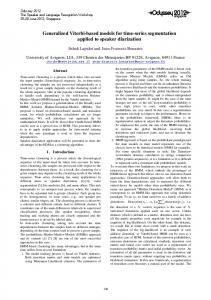
In this study, the AS-GPC was deployed on a validated mechanistic biodiesel (i.e. Fatty Acid Methyl Ester, FAME) transesterification reactor model developed by Mjalli, Lee, Kiew, and Hussain (2009). In addition, the performance of the AS-GPC scheme was benchmarked against that of the A-GPC and GPC schemes. Due to the complex set of chemical reactions as well as the complicated heat and mass transfer characteristics involved, the dynamics of the transesterification reactor is highly nonlinear. Figure 1.2 shows the simplified schematic diagram of the biodiesel production process. As in most chemical plants, the transesterification reactor is the most crucial unit operation to be controlled as it has primary effects on the quality of the

5

biodiesel. The overall reaction for the production of biodiesel in the transesterification reactor is shown here: KOH

⇀ TG + 3MeOH ↽ G + 3FAME

(1.1)

where TG = triglycerides, MeOH = methanol, G = glyceride, and KOH = potassium hydroxide catalyst. This reaction occurs as a sequence of three steps, where TG decomposes to diglycerides (DG) and monoglycerides (MG) with the production of glycerol (G) and FAME, as shown below:

TG + MeOH ⇌ DG + FAME DG + MeOH ⇌ MG + FAME MG + MeOH ⇌ G + FAME

(1.2)

As this work focuses on the development and deployment of the abovementioned advanced controllers on the transesterification reactor model, readers interested in the modeling of the transesterification reactor based on the reactions shown in Eqn. (1.2) are referred to the work of Mjalli, Lee, Kiew, and Hussain (2009).

Transesterification Reactor

Settler Refined Oil

Washing and Purification

Biodiesel

Alcohol Recovery

Alcohol Catalyst Glycerol Glycerol Recovery

Figure 1.2: Simplified schematic diagram of a biodiesel production process. 6

Figure 1.3 shows the strategy by which the AS-GPC scheme was deployed on the biodiesel reactor. The A-GPC scheme used for comparison purpose in this work is a subset of the AS-GPC scheme, where θˆ c in the case of the A-GPC scheme excludes the online computed move suppression weight, indicating model adaptation only in the controller structure. The design of the reactor here is based on one of the available technologies as described in Tapasvi, Wiesenborn, and Gustafson (2004), where the biodiesel reactor is operated below the boiling point of methanol (b.p. = 64.7˚C). The pressure of the reactor is atmospheric and is not controlled. Instead, the temperature of the reactor is controlled to maximize the yield of biodiesel and to minimize the generation of unwanted by-products. Close control of the reactor temperature (i.e. within the range of 5 °C below the boiling point of methanol) is necessary as the rate of reaction increases with increasing reaction temperature (Leung, Wu, & Leung, 2010), but too high a temperature accelerates the saponification reaction of triglycerides (Eevera, Rajendran, & Saradha, 2009; Leung & Guo, 2006). In addition to controlling the reactor temperature, the concentration of the FAME is also controlled to ensure the stability, consistency and the quality of the biodiesel produced. This is important because the concentration of the biodiesel produced in the reactor must lie within the required specifications before proceeding to downstream processing.

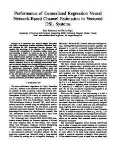
To deal with this, the strategy here as illustrated in Figure 1.3 involves the deployment of two Single Input Single Output (SISO) AS-GPC control loops (ie. a decentralized AS-GPC strategy) to regulate the reactor temperature (T) and the FAME concentration (CME) by manipulating the reactant flow rate (Fo) and the coolant flow rate (Fc) respectively. In addition, four key variables were identified as major disturbances to the biodiesel reactor, viz. the feed temperature (TO), initial concentration of triglycerides (CTGO), coolant inlet temperature (TCO), and stirrer rotational speed (N).

7

Although unable to fully account for the interactions between all variables variab as in the case of a centralized control structure, the decentralized control structure was chosen in this work due to its relative simplicity in design and implementation. Also, the decentralized design is used considering the nature of the tuning correlations correlations employed in this work, which are only applicable for SISO loops. loop

Figure 1.3:: Simplified schematic of the decentralized AS-GPC AS GPC scheme on the biodiesel reactor operating at atmospheric pressure. Fc is the coolant flow rate, Fo is the reactant flow rate, CME is the concentration of FAME, and θˆ c are the controller settings, i.e. the estimated process model parameters and the online computed move suppression weight.

8

1.2 Research Objectives

Following an overview of this research in the previous section, the objectives of this research are:

i) To screen diverse forms of the RLS algorithm for their strengths and weaknesses in tracking time-varying systems, and to select one for implementation.

ii) To perform an open loop dynamic system analysis on the transesterification process for the purpose of studying the nonlinearities and extent of loop interactions in the process.

iii) To perform offline system identification on the various operational regions of the transesterification process in the form of FOPDT model. The results were incorporated into the design of the AS-GPC as a backup and contingency measure.

iv) To design, code and develop the AS-GPC algorithm, where the output of the selected RLS algorithm is used not only for model adaptation in the GPC controller, but also for self-tuning of the move suppression weights by using the analytical tuning expressions proposed by Shridhar and Cooper (1997b).

v) To study the closed loop performance of the AS-GPC scheme in the constraintfree case for the transesterification process and to analyze the locations of the closed loop poles to ensure the soundness and stability of the basic unconstrained controller design.

9

vi) To deploy the newly proposed constrained AS-GPC algorithm on a nonlinear process, i.e. the transesterification process, and testing its performance in servo and regulatory control. Comparisons with the constrained A-GPC, GPC and conventional PID schemes were included where appropriate.

1.3 Structure of Thesis

The remaining six chapters are organized as follows:

a)

Chapter 2 reviews the pertinent literature of this research, i.e. adaptive control, recursive system identification techniques, and the GPC strategy. Furthermore, recent developments in the offline and online tuning methods of the GPC were surveyed, which motivated the AS-GPC scheme. The necessary mathematical background involved in the development of the AS-GPC is also covered.

b)

Chapter 3 discusses the methods used in meeting all the research objectives. In particular, the architecture of the AS-GPC scheme is elaborated.

c)

Chapter 4 presents the results and discussions on the screening of the various RLS algorithms in fulfillment of objective (i), where one specific RLS algorithm was selected for implementation throughout this work.

10

d)

Chapter 5 discusses the results of the open loop dynamic system analysis as well as the results of the offline system identification as stated by research objectives (ii) and (iii).

e)

Chapter 6 is the core of this work, where objectives (iv) - (vi) are delivered. The closed loop performance of the AS-GPC was tested and simulated on a validated mechanistic transesterification reactor model. Necessary analysis and benchmarking with other control schemes were also included to demonstrate the superiority of the newly proposed scheme.

f)

Chapter 7 concludes this research, and proposes future extensions.

11

CHAPTER 2 LITERATURE REVIEW

2.1 Introduction to Adaptive Control

The development of adaptive control was primarily motivated by the growth of the aerospace industry in the 1950’s. However, these initial attempts were mostly unsuccessful (Åström, 1983). The rapid development of adaptive control strategy took place only in the 1970’s, when the design of adaptive controllers was founded on more secure theoretical framework and modern control concepts. Since then, adaptive control has emerged as an active area of research. The rising need for the implementation of adaptive control in the chemical and process industry is in conjunction with the increasing complexity of modern day processes. The use of adaptive control systems was described by Seborg, Edgar, and Shah (1986) as having the capability to “offer significant potential benefits for difficult process control problems where the process is poorly understood and/ or changes in unpredictable ways”. One example of the many complex processes where adaptive control has been widely applied is the polymerization reaction (Seborg, Edgar, & Shah, 1986) where many complex physicochemical phenomena are still poorly understood (Elicabe & Meira, 1988; Mendoza-Bustos, Penlidis, & Cluett, 1990). In addition to this, Seborg, Edgar, and Shah (1986) in their review on adaptive control also reported many other successful adaptive control experimental applications across a wide variety of processes (i.e. absorption/ desorption plants, chemical reactors, distillation columns etc.). Recent applications of adaptive control continue to be reported, e.g. Moon, Cole and Clark (2006), Khodabandeh and Bolandi (2007), Mjalli and Hussain (2009) etc.

12

The extent of coverage on the subject of adaptive control are rather widespread, with several excellent technical review papers (Åström, 1983; Åström, Borisson, Ljung, & Wittenmark, 1977; Seborg, Edgar, & Shah, 1986), books (Åström & Wittenmark, 1994; Clarke, 1981; Ioannou & Fidan, 2006), and tutorial (Isermann, 1982) available in the literature. In these resources, the various types of adaptive controllers available are documented in detail. In addition to these, Anderson and Dehghani (2008) gave a specific review on the different type of challenges present in adaptive control.

The orientation of subsequent sections in this chapter is as follows: First, the different forms of adaptive control strategies available will be addressed, with special attention being given to the self-tuning control strategy. Next, the various components of self-tuning control strategy will be elucidated in detail, viz. the necessary theoretical framework of the various RLS algorithms, the GPC algorithm and the various GPC tuning methods.

2.2 Different Forms of Adaptive Control

Different adaptive control strategies were developed to deal with nonlinearities in the process (Bequette, 1991; Di Marco, Semino, & Brambilla, 1997). Due to the innumerable amount of adaptive control strategies documented in the control literature, here a brief description of the more common adaptive control techniques will be given.

2.2.1

Gain Scheduling

Adaptive control in its simplest form can be implemented by having predetermined sets of controller settings for different operating points of a process

13

(Åström, 1983; Seborg, Edgar, & Shah, 1986). This form of adaptive control strategy, however, does not cater to processes which are time-varying with respect to a specific operating point. A simple implementation of such adaptive control strategy is the ‘gain scheduling’ method (Leith & Leithead, 2000; Rugh, 1991). In gain scheduling, if the process gain (Kp) changes in a predictable manner, the controller settings can be adjusted such that the product of Kp and Kc (the proportional gain) is a constant. In this case, the different values of Kp are predetermined for different operating points of the process, and interpolation is used to obtain the values of Kp in between operating points. Although the gain scheduling method is implementation-wise simple, Wong and Seborg (1986) showed that for a process with a large dead time, the standard gain scheduling based controllers exhibit poorer control of the process than conventional PID controllers. Further, it is not suitable for processes where the dynamics change with time and operational regions (e.g. the time constant and dead time of the process vary with time and operational regions).

2.2.2

Multiple Model Adaptive Control

The simple adaptation strategy as illustrated in Section 2.2.1 can also be extended to cater to model-based controllers. In this case, a number of local LTI models, each representing the dynamics of the process at a specific operating point are predetermined. This form of adaptive control technique is referred to as the Multiple Model Adaptive Control (MMAC). The reason for employing multiple models lies in the fact that a nonlinear process can be approximated by having multiple local LTI models (the more the better), each representing a particular operating region of the process (Banerjee, Arkun, Ogunnaike, & Pearson, 1997). However, due to the practical limits on the number of models feasible for implementation, the approximate dynamics

14

of the process in between the different operating points are usually obtained by some form of scheduling activity (e.g. interpolation). Chow, Kuznetsov, and Clarke (1998), for instance, showed that for predictive control, scheduling can be done by interpolating the poles and zeros of the corresponding local models. Gendron et al. (1993) in their design of a multiple model pole placement controller, weighted the process models based on the output variable. This weighted model was then used to design the pole placement controller. Townsend, Lightbody, Brown, and Irwin (1998) used the prediction error instead as a criterion for weighting the process models. All of these examples utilized the MMAC strategy to design a single controller (i.e. the models are interpolated and weighted and the results are implemented on a single controller). The MMAC strategy can also be implemented in another manner: the controller outputs can be interpolated and weighted instead of the process models (Dougherty & Cooper, 2003a, 2003b; Yu, Roy, Kaufman, & Bequette, 1992). In this case, multiple linear controllers are designed based on the various local LTI models which correspond to different operating points of the process. The control outputs from the various linear controllers are then weighted to produce a control output which is sent to the process. The MMAC approach, although a possible approximation of nonlinear processes, theoretically requires an infinite amount of models to accurately describe a highly nonlinear process. In reality, this is not achievable, giving process and control engineers a hard time in deciding the practical amount of models/controllers to be used. Furthermore, constructing multiple models by offline system identification is cumbersome and requires perturbation of the process from its nominal operating region, which may not be desirable during normal operations. Also, the use of the MMAC approach is restricted to systems which are nonlinear with respect to different operating regions only, and does not include systems which are non-stationary in time with respect to a certain operating region.

15

2.2.3

Model Reference Adaptive System

Another common adaptive control technique is the Model Reference Adaptive Systems (MRAS). This technique was first developed by Whitaker, Yamron and Kezer (1958) for control of aircrafts. Figure 2.1 shows a block diagram of a typical MRAS. In this technique, a reference model is used to specify the ideal response of the process output when subjected to a command signal (uc). The error between the t reference model output (ym) and the real process output (y), which is an indicator of how the real process output deviates from the ideal response, is then used to drive the adjustment mechanism which determines how the controller parameters are changed. changed. In the context of the MRAS, the adjustment mechanism refers to the MIT rule (Osbourne, Whitaker, & Kezer, 1961; Whitaker, 1959). 1959). The associated challenges in implementing this rule (e.g. ( the issue of instability) are given in the recent review of Anderson and Dehghani (2008).

Figure 2.1:: Block diagram of a typical Model Reference Adaptive Systems (MRAS) (adapted from Åström, 1983): 1983) uc is the command signal, u is the process input, y is the process output, and ym is the reference model output.

16

2.2.4

Self-tuning Control

Among the different forms of adaptive control strategies available, the selftuning approach has received the most attention in the past decades (Åström, Borisson, Ljung, & Wittenmark, 1977; Seborg, Edgar, & Shah, 1986; Shah & Cluett, 1991). The basic idea behind the self-tuning approach is to produce a controller which is able to retune itself in real time in order to suit the changing dynamics of the process. Figure 2.2 shows the block diagram of the general self-tuning control framework, where u = process input, y = process output, d1 and d2 = disturbances, and ysp = setpoint. From the figure, given the input and the output of the process, a recursive parameter estimator is used to capture the dynamics of the process online by means of estimating the process model parameters (θp) in the form of a LTI model recursively. Subsequently, based on the preferred choice of control law, θp is then used to calculate the appropriate controller settings (θc) which caters to the most recent process dynamics. This sequence of estimating the process model parameters and retuning of the controller occurs in real time for as long as the process is in operation, which makes this control strategy particularly attractive for controlling difficult time-varying and nonlinear process. Hence, the success of self-tuning control in various processes is evident (Ahlberg & Cheyne, 1976; Bengtsson & Egardt, 1985; Buchholt & Kümmel, 1979; Clarke & Gawthrop, 1981; Corrêa, Corrêa, & Freire, 2002; Ertunc, Akay, Boyacioglu, & Hapoglu, 2009; Hallager, Goldschmidt, & Jorgensen, 1984; Harris, MacGregor, & Wright, 1978; Ho, Mjalli, & Yeoh, 2010a, 2010b; Hodgson & Clarke, 1982; Khodabandeh & Bolandi, 2007; Kwalik & Schork, 1985; McDermott, 1984; Moon, Clark, & Cole, 2005; Moon, Cole, and Clark, 2006; Tingdahl, 2007).

17

Figure 2.2:: Block diagram of the general self-tuning self tuning control framework: u = process input, y = process output, d1 and d2 = disturbances, ysp = setpoint, θp = estimated process model parameters, and θc = controller settings

In the self-tuning tuning control framework, the recursive parameter estimator is a crucial component for capturing the dynamics of the process. Ljung and Söderstöm (1983) provided an in-depth in depth theoretical treatment on the subject of recursive system identification, which is the basic building block for constructing the recursive parameter estimator. Among the he many recursive system identification techniques available in the literature, the RLS algorithm (Ljung, 1987; Ljung & Gunnarsson, 1990; Ljung & Söderstöm, 1983) is the most popular parameter estimation technique used in selfself tuning adaptive control due to its simplicity and rapid convergence converg when properly applied (Seborg,, Edgar, & Shah, 1986; Shah & Cluett, 1991). Since this work focuses mainly on the self-tuning tuning control control strategy, unless mentioned otherwise, the terms ‘adaptive control’ and ‘self-tuning ‘self tuning control’ will be used interchangeably hereafter.

18

Other forms of adaptive control strategies (e.g. gain scheduling, MRAS etc.) will be referred to their respective terms as described previously.

2.3 Recursive System Identification Techniques

As alluded to previously in Section 2.2.4, one of the key components in selftuning control is the recursive parameter estimation, viz. the online process modeling. This technique seeks to overcome the shortcomings of the MMAC approach in approximating the true behavior of a process by estimating the process model parameters of a system recursively in real time. Such an approach is not only equivalent to having a huge models bank with infinite amount of local linear models (without the penalty of exorbitant efforts in constructing these models offline), but also is capable of dealing with time-varying processes.

Among the many recursive identification algorithms available in the literature (Ljung, 1987; Ljung & Söderstöm, 1983), Seborg, Edgar, and Shah (1986) in his comprehensive review on self-tuning control concluded that the RLS algorithm and the Extended Least Squares (ELS) algorithm are the two most frequently employed parameter estimation techniques in adaptive control. However, the RLS algorithm is more popular due to its simplicity and fast convergence when properly applied (Seborg, Edgar, & Shah, 1986). The following subsections are dedicated to address the various theoretical aspects of the RLS algorithms, including the efforts of various researchers in improving the properties of the RLS algorithm.

19

2.3.1

Model Structure

The local dynamics of a general multivariable process can be represented by a Multi Inputs Multi Outputs (MIMO) discrete time Auto-Regressive eXogenous (ARX) model. Consider a MIMO discrete time ARX model with m inputs (uk), n outputs (yk), a bias parameter (dk) and a stochastic noise variable with normal distribution and zero mean (vk):

a ( z −1 ) yk = b ( z −1 ) uk − D + d k + vk

(2.1)

where a[n×n] and b[n×m] are polynomial matrices in the z-domain given as: a ( z −1 ) = I + ∑ i =1 ai z − i

(2.2)

b ( z −1 ) = ∑ i =1 bi z − i

(2.3)

α

β

In Eqn. (2.1), the subscript k is a nonnegative integer which denotes the sampling instance, (k = 0, 1, 2...), D ≥ 0 is the known dead time of the process expressed as an integer multiple of the sampling time (ts), whereas α and β in Eqns. (2.2) - (2.3) are known positive integers and I is the identity matrix. The form of the process model in Eqn. (2.1) can be easily simplified to cater to the SISO case by setting n = m = 1.

It is to be noted that the integers α and β represent the orders of the respective output and input associated polynomials, where having large values of α and β is equivalent to increasing the order of the model. In recursive parameter estimation, having a higher order process model implies an increase in the number of parameters to be estimated, which introduces additional computational burden. On the other hand, having a model order that is too low may not adequately describe the dynamics of the

20

process. Typical values of α and β recommended by Seborg, Edgar, and Shah (1986) are α = 2 or 3 and β = 2 or 3. Alternatively, choosing a valid D value and α = β = 1 would give a FOPDT ARX model, which in many case serves as a good approximation for the purpose of control system design (Seborg, Edgar, & Mellichamp, 2004).

As in all discrete time systems, there is a loss of dynamic information when a continuous process is subjected to sampling operation. Therefore, the sampling time of a discrete time system must be carefully selected to minimize the loss of dynamic information. While having a large sampling time causes slow controller action due to the inadequately sampled data, selecting a small value of sampling time may cause excessive control action and the possibility of the process model exhibiting nonminimum phase behavior (Åström, Hagander, & Sternby, 1984). One possible rule of thumb for selecting the value of sampling time was proposed by Åström and Wittenmark (1997), where the sampling time is selected in terms of the settling time (tsettling) of the process:

tsettling 15

≤ ts ≤

tsettling 6

(2.4)

For FOPDT systems, a good rule of thumb for selecting the sampling time is to select it such that it is approximately one tenth of the process time constant, i.e. ts ≈ 0.1τp (Seborg, Edgar, & Shah, 1986). Other rule of thumbs are also available in the literature, e.g. Middleton (1991).

2.3.2

Recursive Least Squares Algorithm

To capture the dynamics of a slowly time-varying process, RLS algorithm is used for online estimation of the coefficient matrices in a(z-1) and b(z-1) in Eqn. (2.1).

21

With the data of the inputs and the outputs of the process constantly being fed to the RLS algorithm, the RLS seeks to minimize a weighted cost function, V of the form:

Vk = ∑ i =1 λk −i εi k

2 2

(2.5)

where λ ∈ ( 0,1] is the forgetting factor, and εi ∈ ℜn is the vector of prediction error at the i-th instance.

Many variants of the RLS algorithm are reported in the literature (Fortescue, Kershenbaum, & Ydstie, 1981; Kulhavy & Karny, 1985; Mikleš & Fikar, 2007; Park, Jun, & Kim, 1991; Rao Sripada & Fisher, 1987; Salgado, Goodwin, & Middleton, 1988; Shah & Cluett, 1991), with the aim of improving the tracking performance of the conventional RLS algorithm (Ljung, 1987; Ljung & Söderstöm, 1983). The conventional form of the RLS equations is shown here for reference (where λ = 1): ε k = yk − θˆ Tk −1ψ k

(2.6)

γk =

Pk −1ψ k λ + ψTk Pk −1ψ k

(2.7)

Pk =

Pk −1ψ k ψ Tk Pk −1  1 P −  k −1  λ λ + ψ Tk Pk −1ψ k 

(2.8)

θˆ k = θˆ k −1 + γ k ε k

(2.9)

In these equations, γ is the Kalman gain and P is the covariance matrix of the prediction error. The regressor matrix, ψ and the matrix of the estimated process model parameters, θˆ (which in essence is the explicit form of θp mentioned in Figure 2.2) are represented by:

ψT =  − ykT−1 ,..., − ykT−α , ukT− D −1 ,..., ukT− D −β , 1

(2.10)

θˆ T = a1 ,..., aα , b1 ,..., bβ , d 

(2.11)

22

In the conventional RLS algorithm, the forgetting factor, λ is kept constant at unity. This form of the RLS algorithm is best suited for identifying the process model parameters of a LTI system only, and when implemented on time-varying systems, the algorithm loses its adaptivity in the long run. To overcome the shortcomings of the conventional RLS algorithm, a constant forgetting factor of λ ∈ ( 0,1] is employed instead to weigh down older data as the most recent data are more important in a slowly time-varying environment (Ljung, 1987; Ljung & Söderstöm, 1983; Mikleš & Fikar, 2007; Shah & Cluett, 1991). However, it is difficult to select a proper value of the forgetting factor as too small a value would cause the parameter estimates to be very uncertain (i.e. Pk and γk becomes large), whereas a large forgetting factor would cause the algorithm to be insensitive to process parameter changes. With regards to this problem, Fortescue, Kershenbaum, and Ydstie (1981) proposed the use of a timevarying forgetting factor, where the forgetting factor is varied according to the changes in the prediction error. In addition to the time-varying forgetting factor scheme, Cordero and Mayne (1981) suggested an additional mechanism to ensure that the trace of the covariance matrix remains bounded even when there is no new information coming into the RLS algorithm. This algorithm is referred to as the Variable Forgetting Factor Recursive Least Squares (VFF-RLS) and is given here: ε k = yk − θˆ Tk −1ψ k

γk =

Pk −1ψ k 1 + ψ Tk Pk −1ψ k

λk = 1 −

ε Tk ε k σ 1 + ψ Tk Pk −1ψ k 

(2.12) (2.13)

(2.14)

ωk = Pk −1 − γ k ψTk Pk −1

(2.15)

ω λ Pk =  k k  ωk

(2.16)

if trace of ω k λ k ≤ C otherwise

23


(2.17)

where σ/σw is selected to be a large number ≈ 1000 (σw is the variance of any process output measurement noise), while C is a design constant. From Eqn. (2.14), when the prediction error is small, λk → 1. On the other hand, when the prediction error is huge, λk is automatically adjusted to a smaller value (λk < 1). The VFF-RLS scheme has excellent performance in tracking time-varying process model parameters and was successfully implemented on a chip refiner and a paper box machine (Ydstie, Kershenbaum, & Sargent, 1985).

A similar approach was adopted to vary the value of the forgetting factor according to the prediction error of the RLS algorithm in the work of Park, Jun, and Kim (1991), where the equations of the forgetting factor are shown here: λ k = λ min + (1 − λ min ) ⋅ 2 Lk

(2.18)

Lk = − NINT ρεTk ε k 

(2.19)

In Eqns. (2.18) - (2.19), λmin is the minimum forgetting factor, NINT[ i ] is defined as the nearest integer to [ i ], and ρ is a design parameter. Equations (2.6) - (2.9), with (2.18) and (2.19) are referred to as the Exponential Weighting Recursive Least Squares (EWRLS), following Park, Jun, and Kim (1991).

Another interesting approach in identifying time-varying process parameters is to forget only in the direction where new information is coming in (Ljung & Gunnarsson, 1990). This approach was demonstrated by Kulhavý and Kárný (1985) in the Exponential and Directional Forgetting (EDF) algorithm. To speed up convergence in the EDF algorithm, Bittanti, Bolzern, and Campi (1990) proposed an addition of a correction factor referred to as the Bittanti factor to the equation of covariance update. The modified EDF algorithm is shown here: 24

ε k = yk − θˆ Tk −1ψ k

(2.20)

rk = ψ Tk Pk −1ψ k

(2.21)

γk =

Pk −1ψ k 1 + rk

 1− λ λ − rk βk =  1  Pk = Pk −1 −

(2.22)

if rk > 0

(2.23)

if rk = 0

Pk −1ψ k ψTk Pk −1 + δI β k−1 + rk


(2.24)

(2.25)

where δ ∈ [ 0, 0.01] is the Bittanti factor. The value of the Bittanti factor used should be small to avoid over-sensitivity in the EDF algorithm, which could lead to erroneous parameter estimates.

2.3.3

Factorization of the Covariance Matrix

As the various equations of covariance update, i.e. Eqns. (2.8), (2.16) and (2.24), involve subtraction operations, round-up errors due to the limited accuracy of the computer, there is a possibility that the covariance matrix becomes non positive definite. The resulting instability caused by a non positive definite covariance matrix will affect the performance of the RLS algorithm significantly. Hence, to attain numerical stability during implementations of the RLS algorithms, the positive definite feature of the covariance matrix must be retained during recursions. One way to overcome this problem is to use the square root filtering technique (Potter & Stern, 1963), where the covariance matrix is factored as P = SST (in which S is an upper triangular matrix called the square root of P) and subsequent updates of P be accomplished through the factorized component S. Alternatively, Bierman (1976) suggested to use the 25

factorization of P = UDUT, where U is an upper triangular matrix and D is a diagonal matrix. As in the square root filtering technique, instead of updating the covariance matrix directly, the factorized components (i.e. U and D) of the covariance matrix are updated instead. Both methods described above are useful for achieving numerical stability in RLS implementations (Ljung, 1987; Seborg, Edgar, & Shah, 1986), and the choice of factorization method is a matter of preference. In this work, Bierman’s UDUT factorization method is used. Due to the amount of details involved (omitted in the original paper), the rigorous derivation of Bierman’s method is shown in Appendix A.

2.4 Generalized Predictive Control Strategy

The development of modern control concepts in the past decades has led to the emergence of the MPC technology, where an explicit process model is employed within the control algorithm to predict the future behavior of the process response at every time step over a given prediction horizon. An overall concept of the MPC strategy is as illustrated in Figure 2.3. The predicted future output trajectories are then used to compute the optimal sequence of the future input trajectories over a specified control horizon by minimizing the error between the desired future setpoints and the predicted future outputs. From the optimal input sequence, only the first move is eventually implemented in the process. This sequence of calculation is repeated at every sampling time step.

26

Present Past

Future

Process input move to be implemented

Control Horizon, M k

k+1

k+N2

k+2 Prediction Horizon, N2

Legend: Predicted error to be minimized Past (including present) process output Predicted future (excluding present) process output Past (excluding present) process input Optimized future (including present) process inputs

Figure 2.3: The basic concept of Model Predictive Control (MPC).

Excellent reviews and books on the development of various model predictive controllers are available in the literature (Camacho & Bordons, 1999; Garcia, Prett, & Morari, 1989; Qin & Badgwell, 2003; Rossiter, 2003). The different variants of the model predictive controllers in principle share the same basic concept as illustrated in Figure 2.3, with minor differences in the modeling/prediction assumptions involved. Among the many model predictive controllers available in the literature as well as in the industry (e.g. Dynamic Matrix Control, Quadratic Dynamic Matrix Control etc.), the

27

GPC devised by Clarke, Mohtadi, and Tuffs (1987a, 1987b) has attained the status of being one of the most popular MPC algorithms (Clarke, 1988; Garriga & Soroush, 2010). Originally developed for the purpose of adaptive control (in terms of model adaptation without real time adjustment of the tuning parameters), the GPC is known to be a “general purpose” algorithm capable of handling the following process control scenarios (Clarke, Mohtadi, & Tuffs, 1987a) all in one algorithm: •

A non-minimum phase plant

•

An open loop unstable plant or plant with badly damped poles

•

A plant with unknown order

•

A plant with unknown or variable dead time

These properties of the GPC are of significant importance particularly in adaptive control applications when the plant order and dead time are usually unknown. To further illustrate the suitability of implementing the GPC algorithm for adaptive control purposes, Qin and Badgwell (2003) in their excellent review on the practical real world applications of the MPC controllers categorized the GPC under the category of “adaptive MPC algorithms”. In addition, the GPC is proven to show good performance properties and a certain degree of robustness when implemented for the purpose of adaptive control (Clarke, Mohtadi, & Tuffs, 1987a). Figure 2.4 presents the simplified block diagram of the GPC strategy to aid understanding of the subsequent technical discussions. In GPC, the Controlled Auto-Regressive Integrated Moving Average (CARIMA) model is employed for prediction:

a(z

−1

)y

k

= b(z

−1

)u

k −D

+

T ( z -1 ) vk ∆

(2.26)

In Eqn. (2.26), T(z-1) is a design polynomial matrix (Clarke, Mohtadi, & Tuffs, 1987a, 1987b; Yoon & Clarke, 1995), and ∆ = 1 – z-1. When T(z-1) = I, the CARIMA model

28

takes the form of an ARX model with an integrated white noise term for modeling disturbances. Model adaptation in the GPC algorithm is done by having the coefficient matrices of a(z-1) and b(z-1) updated recursively by the RLS algorithm.

To facilitate explanation on the theoretical framework of the GPC algorithm, the symbols and variables used hereafter in this text will follow the conventions developed by Rositter (2003). First, the vector of future and past variables at sampling instance k are defined as:

 yk +1   ∆uk   yk  y   ∆u  y  k +2  k +1  k − 1  ; ∆u =  y = ; y = ; →   k − 1 ⋮  ⋮  →k  ⋮  ←k       ∆uk + M −1   yk −α   yk + N2   ∆uk −1   uk   rk +1  ∆u   u  r k −2 k +2 k +1     ∆u = ; u = ; →r k =  ⋮   → k −1  ⋮  ← k −1 ⋮       rk + N  ∆uk −( D +β ) +1  uk + M −1 

      2 

(2.27)

where the notation of arrows pointing right is used for strictly future (not including current value) vectors and the notation of arrows pointing left for past (including current value) vectors, ∆u is the vector of change in the input variables (i.e. the slew rate), in which the elements are defined as ∆ui = ui – ui-1, and r is the vector of set points. The positive integers N2 and M are the maximum prediction horizon and control horizon respectively, which serve as tuning parameters for the GPC.

29

Figure 2.4:: Simplified block diagram of the conventional GPC strategy. Meaning of symbols: yk = process outputs, y = predicted future outputs, y = past outputs, uk = →k

←k

process inputs, uk - 1 = process inputs at previous instance, ∆uk = first slew rates from the optimized future slew rates, ∆ u

→ k −1

= optimized future slew rates, ∆ u

← k −1

= past slew

rates, r = future setpoints, umax = upper limit of input constraints, umin = lower limit of →k

input constraints, ∆umax = upper limit of slew rate constraints, ∆umin = lower limit of slew rate constraints, N1 = minimum prediction horizon, N2 = maximum prediction horizon, M = control horizon, Ri = 1, …, m = move suppression weights, Wi

= 1, …, n

=

weights on the output residuals, ai = 1, …, α and bi = 1, …, β = coefficients of the polynomial matrix in the CARIMA model, D = discrete dead time.

30

To arrive at the form of model that is useful for predicting the future behavior of the process in the GPC algorithm, the CARIMA model shown in Eqn. (2.26) must first be written in the following form:  y   ∆u  −1 k k−D    + vk A ( z −1 )  = b z ( ) -1 -1  T ( z )   T ( z ) 

( )

(2.28)

( )

where A z −1 = a z −1 ∆ = I + A1 z −1 + ... + Aα+1 z − α −1 .

Since white noise vk has zero mean and can be assumed zero in the future (Rossiter, 2003), with T(z-1) = I, Eqn. (2.28) can be written for N2 steps ahead into the future as shown: CA y + H A y = C b ∆ u →k

←k

→ k −1

+ Hb∆ u

← k −1

(2.29)

The constructions of CA, HA, Cb, and Hb matrices are given in Appendix B. Equation (2.29) can then be rearranged to arrive at the following formulation for prediction:

y = H∆ u + K∆ u + Q y →k

→ k −1

←k −1

←k

(2.30)

where H = C A−1Cb , K = C A−1 H b , and Q = − C A−1 H A . Suffice to note here that N − N × α+1 H ∈ℜ( N 2 − N1 )×M , K ∈ℜ( N2 − N1 )×( D +β−1) , and Q ∈ℜ( 2 1 ) ( ) . In this equation, the

minimum prediction horizon N1 is introduced, and consequently the value of the control horizon M should be lesser or equal to (N2 – N1) in order for Eqn. (2.30) to be valid.

To compute the optimal sequence of future input trajectories, the GPC control law can be obtained by considering the following cost function: T

T     J =  r − y  W  r − y  + ∆ u R∆ u → → → → k −1 k k k −1 →k  →k   

 n×( N 2 − N1 )  ×  n×( N 2 − N1 ) 

In Eqn. (2.31), W ∈ ℜ 

(2.31) and R ∈ ℜ ( m× M )×( m× M ) are positive definite

diagonal weighting matrices defined as: 31

W 0 W = ⋮  0

0 R 0 ⋯ 0  W1 0 ⋯ 0   0 R ⋱ ⋮    ⋱ ⋮  0 W2 ⋱ ⋮ ;   ;W = ; R= ⋮ ⋱ ⋱ 0 ⋮ ⋱ ⋱ 0 ⋱ ⋱ 0      ⋯ 0 W  0 ⋯ 0 R  0 ⋯ 0 Wn 

0 W

⋯

 R1 0 ⋯ 0  0 R ⋱ ⋮  2 ; R= ⋮ ⋱ ⋱ 0    0 ⋯ 0 Rm 

(2.32)

where the diagonal elements of the matrix W consists of the weights ܹ௜ୀଵ,…,௡ for output residuals, whereas the diagonal elements of the matrix R consists of the move suppression weights ܴ௜ୀଵ,…,௠ for changes in inputs. These weights are tunable parameters for obtaining good performance in the GPC controller. In the original GPC algorithm devised by Clarke, Mohtadi, and Tuffs (1987a), however, Wi = 1 (i.e. W = I ) was imposed on the GPC cost function and the same will be used in this work for simplicity and to reduce the amount of tuning parameters involved.

For the unconstrained GPC, the solution to

∂J ∂∆ u

= 0 in Eqn. (2.31) with

→ k −1

W = I yields the following unconstrained GPC control law:

(

∆uk = e1T H T H + R

)

−1

  HT r − Q y − K∆ u  → ← k k − 1 ←k  

(2.33)

where e1T = [ I m×m , 0, 0,..., 0 ]m×mM .

In the unconstrained GPC, it is possible to derive the closed loop transfer function for the purpose of evaluating the closed loop poles. To do this, Eqn. (2.33) is first rewritten in the following form:

∆uk = Pˆk r − Nˆ k y − Dˆ k ∆ u →k

←k

← k −1

(2.34)

32

where:

(

)

(

)

(

)

Pˆk = e1T H T H + R

Nˆ k = e1T H T H + R Dˆ k = e1T H T H + R

−1

HT

−1

−1

HTQ

(2.35)

HT K

Defining the components of Eqn. (2.35) as in Eqn. (2.36), Eqn. (2.34) can be rewritten as Eqn. (2.37): Pˆk =  Pˆk + N1

Pˆk + N1 +1

Pˆk + N1 + 2 ⋯ Pˆk + N2 

Nˆ k =  Nˆ k

Nˆ k −1

Nˆ k − 2 ⋯ Nˆ k −α 

Dˆ k =  Dˆ k −1 

Dˆ k − 2

Dˆ k −3 ⋯ Dˆ k − D+(1−β)  

∆uk = Pˆk ( z ) rk − Nˆ k ( z −1 ) yk − Dˆ k ( z −1 ) ∆uk

(2.36)

(2.37)

where:

Pˆk ( z ) = Pˆk + N1 z N1 + Pˆk + N1 +1 z N1 +1 + Pˆk + N1 + 2 z N1 + 2 + … + Pˆk + N2 z N2 Nˆ k ( z −1 ) = Nˆ k + Nˆ k −1 z −1 + Nˆ k −2 z −2 + … Nˆ k −α z −α

(2.38)

− D + 1−β Dˆ k ( z −1 ) = Dˆ k −1 z −1 + Dˆ k −2 z −2 + Dˆ k −3 z −3 + … + Dˆ k − D+(1−β) z ( )

Rearranging Eqn. (2.37) gives the following:  I + Dˆ k ( z −1 )  ∆uk = Pˆk ( z ) rk − Nˆ k ( z −1 ) yk  

(2.39)

From Eqn. (2.1), ignoring the stochastic components (i.e. the bias parameter and the noise term), it can be shown that: −1

yk =  a ( z −1 )  b ( z −1 ) z − D uk

(2.40)

33

Substituting Eqn. (2.40) in Eqn. (2.39) yields:

uk = b ( z −1 ) z − D 

−1

{

−1

 I + Dˆ k ( z −1 )  ∆ b ( z −1 ) z − D  + Nˆ k ( z −1 ) a ( z −1 )       

}

−1 −1

Pˆk ( z ) rk (2.41)

Hence, the closed loop transfer function is obtained in a straight forward manner by utilizing Eqn. (2.41) in Eqn. (2.40):

yk = a ( z −1 ) 

−1

{

−1

 I + Dˆ k ( z −1 ) ∆ b ( z −1 ) z − D  + Nˆ k ( z −1 ) a ( z −1 )       

}

−1 −1

Pˆk ( z ) rk

(2.42)

where the closed loop poles are given by the solution to the following characteristic equation:

(

det  I + Dˆ k ( z −1 )  ∆ b ( z −1 ) z − D  + Nˆ k ( z −1 ) a ( z −1 )  −1

−1

)=0

(2.43)

The straightforward solution to the GPC cost function and the derivation of the GPC closed loop transfer function as described above are only possible with the unconstrained GPC. For the constrained GPC, the cost function J is minimized with respect to ∆ u

→ k −1

umin ≤ u

→ k −1

while satisfying the following constraints:

≤ umax

∆umin ≤ ∆ u

→ k −1

≤ ∆umax

(2.44)

The optimal sequence of the future input trajectories is then obtained by rearranging and solving Eqn. (2.31) in the form of a Quadratic Programming (QP) problem (given W = I ):

34

1

min  2 ∆ u

T

→ k −1

B∆ u

→ k −1

  → k −1 

+ gT ∆ u

∆u

→k −1

Subject to Ω∆ u

→ k −1

(2.45)

−µ ≤ 0

where B and g are defined as (Rossiter, 2003): B = HT H + R

  g = HT K∆ u + Q y − r  → ← k k − 1 ←k  

(2.46)

The matrices Ω and µ in Eqn. (2.45) can be obtained by formulating Eqn. (2.44) in the form of linear inequalities, of which the details can be found in Camacho and Bordons (1999), Maciejowski (2002), and Rossiter (2003). The solution to the QP problem in Eqn. (2.45) yields the optimal future input trajectories, where only the first move is implemented in the process.

Regarding stability in the constrained case, although it can be guaranteed by parametric interpretations and the use of the well-known “dual-mode” algorithms with guaranteed convergence (Rossiter, 2003), in terms of evaluating stability by means of the closed loop poles, there has not been any possibility of doing so for the constrained GPC. Thus, this work considers only the stability in the unconstrained case through its closed loop transfer function. Despite the fact that stability in the unconstrained case does not guarantee stability in the constrained case, it is still worth doing a study in the stability of the former scenario (Rossiter, 2003) because if the control law in the unconstrained case does not give good performance, the corresponding constrained case cannot be expected to give good performance.

35

2.5 Generalized Predictive Control: Tuning Methods

As alluded to in the previous section, the GPC algorithm has several tuning parameters which can be adjusted to affect the performance of the controller. For ease of reference, the tuning parameters are recapitulated here: a) Minimum prediction horizon (N1) b) Maximum prediction horizon (N2) c) Control horizon (M) d) Move suppression weight (Ri)

Over the decades, many authors had proposed different formulations and strategies to tune the GPC controller. In a recent work, Garriga and Soroush (2010) presented a review on the various MPC (i.e. GPC and DMC) tuning methods available, with a specific section dedicated specifically to the subject of “auto-tuning” (synonymous to “self-tuning” in the context of this work). In the following subsections, a brief review on the various offline GPC tuning methods is given, followed by discussions on the developments of self-tuning methods.

2.5.1

Minimum and Maximum Prediction Horizons (N1 and N2)

In general, the value of N1 in the GPC formulation is set to 1 if the dead time of the plant is not known a priori as selecting a value of N1 much greater than the dead time of the plant will cause the controller to ignore the dynamics of the plant within the (N1 - dead time) horizon. This may cause the controller performance to deteriorate since the ignored dynamics can be crucial in determining the appropriate control output. As such, the value of N1 = 1 is a conservative choice if nothing is known about the dead

36

time of the process (Banerjee & Shah, 1992; Clarke, Mohtadi, & Tuffs, 1987b; McIntosh, Shah, & Fisher, 1989, 1991). Conversely, if the discrete dead time of the plant is known a priori, N1 can be selected as equal to (discrete dead time + 1) to minimize computations (Camacho & Bordons, 1999; Clarke, Mohtadi, & Tuffs, 1987a). Other tuning guidelines for selecting the minimum prediction horizon based on the order of a(z-1) and ࢈∗ (z-1) [where ࢈∗ (z-1) = z-Db (z-1)] are also available in the literature (Clarke & Mohtadi, 1989; McIntosh, Shah, & Fisher, 1989, 1991).

As for N2, in order to guarantee the stability of the closed loop system, its value should be set to infinite (Camacho & Bordons, 1999; Maciejowski, 2002; Rossiter, 2003), which in practical terms would mean setting N2 to large values. If a finite value for N2 is selected, its value should be carefully chosen based on tuning guidelines to ensure the closed loop stability of the system. Clarke, Mohtadi, and Tuffs (1987a) proposed setting the value of N2 between the order of ࢈∗ (z-1) and the discrete rise time of the process. In another work, Clarke and Mohtadi (1989) proposed that the value of N2 be chosen based on a rise time of 95 % of the process steady state. A more explicit tuning correlation was proposed by Shridhar and Cooper (1997b) for the selection of N2 for SISO FOPDT systems:

 τ   N 2 = CEIL 5  p  + D    ts  

(2.47)

where τp is the process time constant and CEIL[ i ] is defined as the nearest next integer to [ i ]. Although Eqn. (2.47) was originally developed for the tuning of DMC, the authors claimed that the same equation can be also used for tuning the GPC. Many other tuning guides had been proposed for the selection of N2 (Banerjee & Shah, 1992; McIntosh, Shah, & Fisher, 1989, 1990, 1991; Trierwieler & Farina, 2003; Yamuna & Unbehauen, 1997), however, the general agreement is that N2 should be sufficiently

37

large to cover the important parts of the step response curve (Mikleš & Fikar, 2007) as well as to ensure the stability of the closed loop system.

2.5.2

Control Horizon (M)

In the GPC formulation, selecting a value of M = 1 produces a conservative controller, whereas values of M > 1 produces a more robust controller at the cost of increased computation load. Several authors have proposed to set the value of M = 1 (Banerjee & Shah, 1992; Clarke & Mohtadi, 1989; Clarke, Mohtadi, & Tuffs, 1987a, 1987b; McIntosh, Shah, & Fisher, 1989, 1991; Yamuna & Unbehauen, 1997). Other than that, Clarke and Mohtadi (1989) proposed that M be equated to the discrete dead time of the process, whereas McIntosh, Shah, and Fisher (1989, 1991) proposed that M be chosen based on the order of a(z-1) plus one. In his book on MPC, Rossiter (2003) stated that “a value of M ≥ 3 often seems to give performance close to the global optimal”. Other prediction horizon based and stability based tuning rules for selecting the value of M in the GPC framework are available in the work of Rawlings and Muske (1993) as well as in the work of Trierwieler and Farina (2003). In general, the guidelines given by these authors suggest that the value of M should not be overly large. Furthermore, the control horizon does not have significant effects on the closed loop performance in the presence of move suppression (Shridhar & Cooper, 1997b), which is the reason for the authors’ proposal of the values of M between 1 to 6.

2.5.3

Move Suppression Weight (Ri)

The move suppression weight, also known as the move suppression coefficient, is used to penalize the slew rates such that a larger penalty produces a more robust but

38

sluggish controller. Conversely, selecting a small value of Ri or a complete absence of move suppression produces an aggressive but less robust controller. This section shall be restricted to the more common methods of tuning Ri (Garriga & Soroush, 2010) and shall not cover the concepts deployed in algorithms such as the Predictive Functional Control etc (Rossiter, 2003). Several authors have proposed to select the value of Ri based on actual control performance, i.e. trial and error (Karacan, Hapoglu, & Alpbaz, 2001; McIntosh, Shah, & Fisher, 1989, 1991). In these studies, the strategies used by the authors involved making Ri the single active tuning parameter, while all other tuning parameters were fixed. This strategy concurs with the perspective of optimal feedback control (e.g. the Linear Quadratic Regulator, LQR), where the weights of the objective function to be minimized are the sole tuning parameters of the controller (Mikleš & Fikar, 2007). Clarke and Mohtadi (1989) suggested setting the value of Ri = 0. However, if numerical stability is an issue of concern, the authors proposed to adopt values of Ri ≈ 0. Banerjee and Shah (1992) suggested choosing values of Ri in the range between 1 - 2. Yamuna and Unbehauen (1997) proposed to tune the move suppression weight based on the following relationship: Ri = κN 2 + π

(2.48)

where κ and π are constants determined from past Ri and N2 values. Using this relationship, Ri is recalculated each time N2 is retuned based on the performance tuning procedure proposed by McIntosh, Shah, and Fisher (1990).

In another tuning formulation by McIntosh, Shah, and Fisher (1989), the authors proposed that an initial guess for the “relative control weighting (ܴ௜∗ )” be calculated based on trace(HTH) and subsequent values of Ri be calculated based on the relationship of Ri = ܴ௜∗ ࢈∗ (1). In addition, the value of ܴ௜∗ can be fine-tuned during operation to improve the overall performance. Most of the methods described to this juncture are not

39

suitable for RLS-based self-tuning purposes due to the lack of association between the tuning guides and the process model parameters. Shridhar and Cooper (1997b) in their attempt to tune Ri based on the process model parameters of an open loop stable SISO FOPDT model proposed the following analytical expressions to calculate its value: Ri = f K 2p

(2.49)

where:

0 M =1   f =  M  3.5τp ( M − 1)   500  t + 2 − 2  M > 1  s  

(2.50)

Equations (2.49) - (2.50), although developed originally for unconstrained DMC, can also be directly applied for tuning the Ri in the GPC (Mikleš & Fikar, 2007). The authors also proposed to select the usual values of M ranging from 1 to 6 when these expressions are applied. Since Eqns. (2.49) - (2.50) are developed based on a process model and are relatively easy to implement, the self-tuning component in the AS-GPC proposed in this work shall be designed based on these equations. As to the success of this tuning strategy, several researchers had obtained good results with it (Nithya, Gour, Sivakumaran, Radhakrishnan, & Anantharaman, 2007; Tahami & Ebad, 2009; Villanueva Perales, Ollero, Gutierrez Ortiz, & Gomez-Barea, 2009). However, in the review of Garriga and Soroush (2010), the authors concluded that this tuning strategy yielded faster response at the expense of more aggressive controller moves. To what extent this conclusion holds true when the tuning strategy is deployed in a recursive fashion, remains a question to be answered in Chapter 6 of this thesis.

2.5.4

Self-Tuning Methods

In these methods, tuning of the GPC is not done offline by control engineers, but rather, the controller automatically retunes itself in real time. As the effect of an 40

individual tuning parameter strongly depends on the settings of the other tuning parameters in the GPC controller (McIntosh, Shah, & Fisher, 1991), the task of controller tuning is not straightforward for an inexperienced control engineer. Hence, with the implementations of self-tuning strategies, minimal knowledge is required of the control engineer to initiate the tuning procedure.

In the literature, although the majority of the developments in self-tuning of the MPC were tailored specifically for the DMC, in general the same principle can be applied on the GPC. In the work of Al-Ghazzawi, Ali, Nouh, and Zafiriou (2001), the authors developed analytical sensitivity expressions relating the process outputs and the DMC tuning parameters (i.e. the weights on the output residuals and the move suppression coefficients) and utilized it for automatic online adjustments of the tuning parameters. The prediction and control horizons were set at predetermined values and only the weights on the output residuals and the move suppression weights were retuned in real time. Han, Zhao, and Qian (2006) proposed a self-tuning strategy based on Particle Swarm Optimization (PSO). A novel performance index was developed and PSO was used to search for the optimal tuning parameters while minimizing the performance index to cater to the worst operating conditions. Kawai et al. (2007) applied this method to tune the DMC. However, instead of computing the entire set of tuning parameters online, the optimization problem was restricted to computing the optimal values of the inputs and outputs weights only, hence reducing the computation load required. Ali and Al-Ghazzawi (2003) presented a self-tuning scheme based on fuzzy logics. In this scheme, the prediction horizon, the move suppression weights, and the weights of the output residuals were determined from predefined fuzzy rules which formulate the general tuning guides reported in the literature, while the control horizon was fixed at a constant value. As for the GPC, Liu and Wang (2000) proposed two

41

algorithms to carry out a multi-objective optimization for the purpose of obtaining the optimal set of tuning parameters as well as to optimize the control moves online. In a recent work for the GPC implemented through the Programmable Logic Controller (PLC), Valencia-Palomoa and Rossiter (2010) suggested to auto-tune the GPC based on estimates of model behavior as compared to standard second order characteristics (i.e. rise time, settling time, overshoot, process gain, dead time and sampling time of the process) of the process. In all these studies, a static internal model was employed for the predictive controller, and no model adaptation scheme was adopted explicitly. This work attempts to incorporate both the model adaptation and self-tuning strategies in the GPC controller by using the output of the RLS algorithm, of which the details are given in Section 3.6. To what extent the performance of the controller can be improved (if there is any at all), remains a question to be answered in this work.

42

CHAPTER 3 RESEARCH METHODOLOGY

3.1 General Remarks

In this chapter, only the necessary procedures and methods used to meet the objectives of the research will be elucidated in detail, while the results of the respective sections are presented in the subsequent chapters. Unless mentioned otherwise, all simulations involved in this work were programmed using Simulink® version 7.1 of MATLAB® program version R2008a. Where the use of S-function in Simulink® is involved, the programs were coded as an M-file to be embedded within the S-function block. The use of MATLAB toolboxes where applicable will be highlighted in the sections concerned.

3.2 Coding and Screening of Various RLS algorithms

Selected RLS algorithms with Bierman’s UDUT factorization were coded as Sfunctions. An example code of the RLS algorithm, specifically the VFF-RLS algorithm, is given in Appendix C. To ensure proper and correct coding, the conventional RLS algorithm was first coded and implemented on a simple LTI model, with fixed process model parameters. The results obtained, viz. the estimated process model parameters from the simulation was validated with the results obtained from the sample program (which also utilizes the conventional RLS algorithm) given by Mikleš and Fikar (2007). The covariance matrix and the prediction error of the identification were also validated against those obtained from the sample program. Upon successful validation of the coded conventional RLS algorithm, other variants of the RLS algorithm were obtained 43

by slight modification of the code for the conventional RLS algorithm. The simulation results obtained by using the modified RLS algorithms should not differ much from those obtained from the conventional RLS algorithm, since the system involved here is linear time invariant, and these modifications of the RLS algorithm only show significant differences in performance when the system being identified is time-varying.

To test the performance of the various RLS algorithms in identifying timevarying systems, a hypothetical, stable, discrete time LTI transfer function in the zdomain was used as the process model:

Gp ( z ) =

0.6 z −1 + 0.7 z −2 + 0.8 z −3 + 0.9 z −4 + 1.0 z −5 1 + 0.1z −1 + 0.2 z −2 + 0.3z −3 + 0.4 z −4 + 0.5z −5

(3.1)

In Eqn. (3.1), there are altogether ten parameters to be identified. This number of parameters was chosen to make system identification more difficult in order to challenge each RLS algorithm. To simulate a process model where the process model parameters are time-varying, the process model parameters, which consist of random and arbitrary values but resemble a stable plant, were varied abruptly at the 70th time step as follows:

0.1z −1 + 0.9 z −2 + 1.5 z −3 − 0.2 z −4 − 0.3z −5 Gp ( z ) = 1 + 1.1z −1 + 0.8 z −2 + 0.6 z −3 + 0.7 z −4 + 0.3z −5

(3.2)

To ensure that the system is sufficiently excited, white Gaussian noise with zero mean and variance of 0.1 was used as an input to the system, while the same noise type with a variance of 0.01 was added to the output of the system to simulate a noisy environment. The Euclidean norm of the parameter error, L2 =|| θ 0 − θˆ ||2 at every time step was calculated and plotted against time, where θ0 is the vector of parameters which contains the true values of the process model parameters, as shown in Eqns. (3.1) and (3.2), and θˆ is the vector of estimated parameters. Based on the Euclidean norm of the 44

parameter error, the convergence and the steady state parameter mis-adjustment error of the various RLS algorithms were analyzed to explore the strengths and weaknesses of each algorithm. Based on the screening results, one of the RLS algorithms was selected for self-tuning control implementations in this work.

3.3 Coding of the Generalized Predictive Controller

The GPC algorithms (excluding the quadratic programming solver) for both the unconstrained and the constrained versions were coded as S-functions. For the constrained GPC, in order to solve the quadratic programming problem online at every time step, the subroutine ‘quadprog’ under the Optimization ToolboxTM was used with the default settings retained.

For validation purposes, assuming the knowledge of the internal GPC model used, e.g. a first order CARIMA model, it is possible to manually determine the numerical values of CA, HA, Cb, and Hb matrices (as shown in Appendix B), which eventually can be used to determine the H, K, and Q matrices as shown in Eqns. (2.29) (2.30). These manually determined results were used to validate the results obtained from the coded GPC algorithm. The S-functions for the unconstrained and constrained GPC algorithm and its variants developed here are shown in Appendix D and E respectively. Although decentralized controllers were designed in this work, the GPC algorithm coded here can handle multivariable control problems, as shown in one of the author’s publications (Ho, Mjalli, & Yeoh, 2010a).

45

3.4 Open Loop Dynamic System Analysis of the Biodiesel Reactor

Open loop dynamic system analysis of the transesterification reactor model was done for the following reasons: a) To show the nonlinearities exhibited by the transesterification process, hence justifying the need for an advanced control algorithm to be implemented. b) To use the data of the open loop response for the transesterification process for offline system identification, where the parameters of a FOPDT model were estimated. The estimated model parameters were then used in the design of the control schemes presented in this work.

To study the open loop transients of the transesterification process, the manipulated variables (i.e. Fo and Fc) were increased in small steps across the respective operating ranges by manipulating the control valve openings. For ease of reference, the control valves for manipulating Fo and Fc were termed CV-101 and CV-102 respectively. In the work of Mjalli, Lee, Kiew, and Hussain (2009), loop pairings were done by using the Relative Gain Array (RGA) analysis, where Fo was paired against CME, while Fc was paired with T. With these pairing results retained, it is of interest in this study to show via the open loop transients the nonlinearities involved in the transesterification process as well as the extent of the process interactions observed. Series of step changes in the valve stem positions of CV-101 and CV-102 (which in turn manipulate Fo and Fc) were designed and introduced to the process in the manner as shown in Table 3.1. The values of the valve stem positions can be of any arbitrary numbers spanning from 0 % to 100 %, but since the nominal valve stem positions of CV-101 and CV-102 for the biodiesel reactor are 17 % and 26.8 % respectively, it is more convenient to choose combinations that step through these values.

46

Table 3.1: Trends of step changes in the valve stem positions of CV-101 and CV-102 at every time interval of 3000 s. The control valves fully shut and fully open at 0 % and 100 % respectively.

Valve Stem Position for

Valve Stem Position for

CV-101 (%)

CV-102 (%)

1

7 : +10 : 97

26.8

2

97 : -10 : 7

26.8

3

17

6.8 : +10 : 96.8

4

17

96.8 : -10 : 6.8

5

7 : +10 : 97

6.8 : +10 : 96.8

6

7 : +10 : 97

96.8 : -10 : 6.8

7

97 : -10 : 7

6.8 : +10 : 96.8

8

97 : -10 : 7

96.8 : -10 : 6.8

Simulation

Referring to simulation 1 from the table, the valve stem position for CV-101 was set at 7 % in the beginning of simulation (to be varied afterwards), while maintaining a constant valve stem position of 26.8 % for CV-102 throughout the entire simulation. Upon achieving steady state of the output variables, a positive step change of 10 % in the valve stem position for CV-101 was introduced at 3000 s. Subsequent introductions of positive step changes of the same magnitude were done at intervals of 3000 s until the valve approaches its high operating range at 97 %. The open loop transients of the input (i.e. Fo and Fc) and output (i.e. CME and T) variables as well as the corresponding valve stem positions were then recorded. It is important to note that the time duration of 3000 s selected was sufficiently long to capture the open loop transients of the process after every step change and the output variables were able to achieve steady states within the given time duration. In simulation 2, instead of having an ascending trend in

47

the valve stem position for CV-101, step changes of the same magnitude in the opposite direction (i.e. from 97 % to 7 %) were introduced.

In simulations 3 and 4, the same procedures as in simulations 1 and 2 were used to study the effect of the valve stem position for CV-102 on the output variables. The valve stem position for CV-101 was maintained at 17 %, while step changes of opposite directions were introduced on separate runs (i.e. the positive step changes for simulation 3 and the negative step changes for simulation 4) across the entire operating range of the valve (6.8 % - 96.8 %). In simulations 5 – 8, instead of only manipulating a single input as in simulations 1 – 4, a series of step changes was introduced to both inputs simultaneously in a fashion similar to the 22 factorial design, where all possible combinations of step changes in the ascending and descending trends were considered. The open loop transients in these experiments were important to show the nonlinearities and process interactions observed under all possible combinations of input perturbations.

3.5 Offline System Identification of the Biodiesel Reactor

As alluded to in Section 3.4, the data of the open loop transients are useful for offline system identification where simple LTI transfer function models can be identified and used in control design purposes. In this study, the FOPDT model was chosen as the model structure for system identification (the reasons for this choice will be elaborated in the following section). Although the biodiesel reactor is a multivariable process, for simplicity, system identification was performed in a decentralized fashion, where only Fo – CME and Fc – T relationships were modeled, thus omitting the possible process interactions involved. The iterative prediction-error minimization method (Ljung, 2008), denoted by the ‘pem’ subroutine under the System Identification

48

ToolboxTM, was used to estimate the model parameters of a FOPDT model with a maximum allowable estimated dead time of 100 s. Since it is of interest in this study to identify individual SISO models, the data from simulations 1 and 3 in Table 3.1 were used for achieving this purpose. The estimated Kp, τp, and θd (i.e. dead time) were recorded and the R2 (i.e. coefficient of determination) of the model fit was computed.

3.6 Advanced Control System Design for the Biodiesel Reactor

In this work, it is of interest to study the performance of the AS-GPC scheme as compared to the A-GPC and GPC schemes. The GPC scheme in this case is the conventional GPC algorithm without model adaptation or self-tuning. Before exploring the performances of these schemes under closed loop conditions on the transesterification reactor, the control architecture of the various schemes under consideration must be clearly defined. For all schemes, two controllers were designed, one for the Fo - CME loop and the other for the Fc - T loop. It should be noted that the procedures here are general and applicable to both the unconstrained and constrained versions of the particular control scheme under discussion.

The conventional GPC scheme differs from the AS-GPC and A-GPC schemes in that no RLS algorithm is involved. The model parameters used in the GPC remained unchanged throughout its entire implementation and were obtained by converting the continuous time model parameters (i.e. from the offline system identification outlined in Section 3.4) to the corresponding discrete version using Eqns. (3.3) - (3.5) (Seborg, Edgar, & Mellichamp, 2004):

 t  a 1 = − exp  − s   τp 

(3.3)

49

  t b 1 = K p 1 − exp  − s  τ  p 

    

θ  D = CEIL  d   ts 

(3.4)

(3.5)

The sampling time ts selected for both CME and T loops were based on the values of τp identified around the nominal operating conditions as outlined in Section 3.4, where ts ≈ 0.1τp according to rule of thumb (Seborg, Edgar, & Shah, 1986). Values of θd were also obtained from the offline system identification around the nominal operating conditions. In the GPC scheme, the controller tuning parameters were calculated by using Eqns. (2.49) - (2.50) proposed by Shridhar and Cooper (1997b).

As opposed to the GPC scheme where no RLS algorithm is needed, for each separate control loop in the AS-GPC and A-GPC schemes, the screened and selected RLS algorithm by using the procedures outlined in Section 3.2 was used to identify the process model parameters of a SISO first order ARX model, which would then be incorporated in the CARIMA representation to be used for prediction in the controller. The reasons for identifying the process model parameters of a SISO first order ARX model, which can easily be recast in the form of a FOPDT model (i.e. ignoring the bias parameter and the noise term), are obvious: i)

The FOPDT model is a widely used model structure for control design purposes and often serves as a reasonable approximation for the dynamics of most processes (Seborg, Edgar, & Mellichamp, 2004).

ii)

Tuning correlations based on the FOPDT model for predictive controllers are available (Shridhar & Cooper, 1997b), which can be conveniently adapted to design the AS-GPC controller.

50

Table 3.2 shows the necessary parameters to be defined in the SISO ARX model for each loop to cater for parameter estimation purposes. Among the parameters shown, the values of n, m, α and β were determined in a straightforward manner based on the structure of the model chosen (i.e. a SISO first order ARX model). As for the values of D and ts, both were determined in the same manner as described for the GPC scheme.

Table 3.2: Parameters of the discrete time SISO ARX model which must be defined for parameter estimation purposes, both for the FAME concentration (CME) and the reactor temperature (T) loops.

Parameter

Symbol

Unit

Number of outputs

n

-

Number of inputs

m

-

Order of a(z-1)

α

-

Order of b(z )

β

-

Discrete dead time

D

-

Sampling time

ts

s

-1

Prior to coupling the screened and selected RLS algorithm (as outlined in Section 3.2) to the GPC algorithm for the design of the AS-GPC and A-GPC schemes, the parameters associated with the specific form of the RLS algorithm (e.g. σ and C for the VFF-RLS algorithm etc.) chosen for control system design must be determined. Readers are referred to Subsection 2.3.2 for more information on the parameters. Figures 3.1 and 3.2 show the adaptive strategies used in the AS-GPC and the A-GPC schemes respectively. In both the AS-GPC and the A-GPC schemes, the RLS algorithm estimates the process model parameters of a SISO first order ARX model, viz. a1 and b1, for both the CME and T loops, which will then be incorporated in the CARIMA representation as shown in Eqn. (2.26) for use in the controller. Ignoring the stochastic

51

components (i.e. the bias parameter and the noise term), the SISO first order ARX model can be recast in the following form, which in essence is a representation of a discrete time FOPDT model:  b z −1 z − D  yk =  1 u −1  k  1 + a1 z 

(3.6)

Generally, for any particular system to be stable, the poles must lie within the unit circle of the z-plane, i.e. |z| < 1 (Seborg, Edgar, & Mellichamp, 2004). Before the estimated SISO ARX model parameters can be passed to the GPC for model adaptation in the SISO CARIMA model or self-tuning purposes, the pole of the identified model (i.e. z = -a1) was screened to ensure that the identified model had stable dynamics (since the transesterification reactor is an open loop stable process). In the case of a FOPDT model, the stability domain can be further simplified. To do this, consider the continuous time domain equivalent of Eqn. (3.6) given in Eqn. (3.7), which can only be stable, if τp > 0:

 K p e−θd s  y ( s) =  u s  τ s + 1  ( ) p  

(3.7)

Since the values of τ p ∈ ℜ and ts ∈ℜ must be positive for all real physical processes, imposing the conditions of τp > 0 and ts > 0, a1 in Eqn. (3.3) can only take on negative real values. Knowing z = -a1 for the particular system described by Eqn. (3.6), the criterion for the identified pole to imply stable dynamics is z ∈ (0, 1) or a1 ∈ (-1, 0). Hence, the poles of the identified model for the AS-GPC and A-GPC schemes were screened based on this rule. In short, at any particular time step, if the value of the estimated a1 falls between -1 and 0, the updated a1 and b1 are passed to the GPC; otherwise a backup model previously identified from Section 3.5 and converted to its discrete time equivalent using Eqns. (3.3) - (3.5) are used in the controller. This is

52

further illustrated in Figures 3.1 - 3.2, where for both the A-GPC GPC and AS-GPC AS schemes, Route 1 is implemented on the basis of stable dynamics of the identified model, while Route 2 is implemented as a contingency option should the identified model be unstable.

Figure 3.1: The adaptive strategy used in the A-GPC A scheme. Pole screening dictates whether Route 1 or Route 2 is implemented at every time step.

53

Figure 3.2: The adaptive strategy used in the AS-GPC scheme. Pole screening dictates whether Route 1 or Route 2 is implemented at every time step.

For the A-GPC GPC scheme, the estimated process model parameters were used only for model adaptation in the GPC controller. In this case, the values of the tuning parameters were chosen based on the guideline summarized in Table 3.3 3. using the value of ts and the nominal values of τp and D selected previously in this section. section Most of the tuning guideliness presented in Table 3.3 were taken from the work of Shridhar and Cooper (1997b) except the one presented for N1, which is a standard guideline guide throughout mostt MPC literature (Camacho & Bordons, 1999). In the A-GPC A scheme, the tuning parameters were fixed throughout the entire closed loop implementation. implementation As for the AS-GPC GPC scheme, the values of N1, N2, M and Ri were initialized in the same manner as described for the A-GPC A scheme. However, ass soon as the RLS algorithm had stabilized, further processing proce of the model parameters were performed to compute the updated move suppression weight for each loop. In this strategy, strategy, the values of N1, N2

54

and M remained unchanged during implementation, leaving Ri as the single active tuning parameter to be manipulated automatically by the controller in real time. For this purpose, simple manipulation of Eqn. (3.3) is needed to solve for τp and Kp at every time step based on the updated value of a1 from the RLS algorithm: τp =

−t s b > 0 as a1 ∈ (-1, 0) and K p = 1 ln ( −a 1 ) 1 + a1

(3.8)

Hence, with values of τp and Kp, Ri can be updated accordingly using the equations developed by Shridhar and Cooper (1997b), i.e. Eqns. (2.49) - (2.50). It is to be noted that Eqn. (3.8) is used only for computing Ri, while the values of N1 and N2 for a certain value of ts were calculated based on the nominal values of τp and D obtained earlier through offline system identification.

Table 3.3: Tuning guideline used in this work for the A-GPC and AS-GPC schemes Tuning Parameter

Symbol

Value

A-GPC

AS-GPC

Min. prediction horizon

N1

D+1

Fixed

Fixed

Max. prediction horizon

N2

Eqn. (2.47)

Fixed

Fixed

Control horizon

M

1-6

Fixed

Fixed

Move suppression weight

Ri

Eqns. (2.49) - (2.50)

Fixed

Adaptive

3.7 Closed Loop Performance Validation and Analysis on the Biodiesel Reactor

Since the tuning correlation proposed by Shridhar and Cooper (1997b) were intended for use with unconstrained predictive controllers, the constraint-free version of the AS-GPC was implemented first on the biodiesel reactor and tested for the ability to track changes in setpoint. The nature of setpoints introduced to the CME and T loops was of magnitudes ±0.1 kmol/m3 and ±2 K around the respective nominal operating conditions. The closed loop poles for the constraint-free AS-GPC were calculated based

55

on Eqn. (2.43) to study the stability of the unconstrained AS-GPC. Following this, the control strategy adopted in the AS-GPC was further pushed to its limits by incorporating constraints [Eqn. (2.44)] to the controller. The constrained AS-GPC scheme was tested for the ability of handling both the servo and the regulatory problems. Furthermore, the performance of the constrained AS-GPC scheme was benchmarked against that of the constrained A-GPC, constrained GPC and conventional PID schemes. The screenshot of the AS-GPC implementation in Simulink® version 7.1 is given in Figure 3.3.

Figure 3.3: Screenshot of AS-GPC implementation in Simulink® version 7.1

The Internal Model Control (IMC) method (Chien & Fruehauf, 1990; Rivera, Morari, & Skogestad, 1986) and the Ziegler-Nichols (ZN) method (Ziegler & Nichols, 1942) as shown in Table 3.4 were used to tune the PID controllers. The selection of the IMC design parameter τc in this work was based on the rule of thumb proposed by Skogestad (2003, 2004), where τc = θd. The CME and T profiles under closed loop

56

conditions using the same setpoint changes as described above were plotted and the various performance indicators were assessed.

Table 3.4: Internal Model Control (IMC) and the open loop Ziegler-Nichols (ZN) based PI and PID controller settings, where Kc = proportional gain, τI = integral time constant, τD = derivative time constant, τc = IMC design parameter, Kp = process gain, τp = process time constant, and θd = process dead time.

Method IMC PI

IMC PID

ZN PI

ZN PID

Model

Kc

K p e −θd s

τp

τp s + 1 K p e −θd s τp s + 1

K p ( τc + θd )

θd 2 θ   K p  τc + d  2 

τI

τD

τp

-

τp +

K p e −θd s

0.9τp

τp s + 1

K p θd

K p e −θd s

1.2τp

τp s + 1

K p θd

τp +

θd 2

τp θd 2τp + θd

3.33θd

-

2.0θd

0.5θd

57

CHAPTER 4 SCREENING OF VARIOUS RLS ALGORITHMS

4.1 Chapter Overview

To screen the various RLS algorithm and to test their performance, the methods outlined in Section 3.2 were used. First, the effects of the various parameters of different RLS algorithms were explored to discover their effects on the sensitivity of different RLS algorithms. Following this, the performance of the various algorithms were compared and analyzed before a decision was made on the selection of the algorithm to be used in this work. To facilitate discussions, the essential differences (i.e. the equations involved for updating the covariance matrix) between the VFF-RLS, EWRLS, and EDF algorithms are given in Table 4.1. For a complete presentation of the equations, readers are referred to Section 2.3.2.

58

Table 4.1: Summary of essential differences between the VFF-RLS, EWRLS and EDF algorithms.

Algorithm

How the Covariance Matrix is Updated

Reference of Equation

1) Select a value for σ, then calculate the forgetting factor, λk: λk = 1 −

ε Tk ε k σ 1 + ψ Tk Pk −1ψ k 

Eqn. (2.14)

VFF-RLS 2) Use λk to update the covariance matrix P:

ωk = Pk −1 − γ k ψTk Pk −1

Eqn. (2.15)

ω λ Pk =  k k  ωk

Eqn. (2.16)

if trace of ω k λ k ≤ C otherwise

1) Select a value for ρ, then calculate the forgetting factor, λk:

EWRLS

Lk = − NINT ρεTk ε k 

Eqn. (2.18)

λ k = λ min + (1 − λ min ) ⋅ 2 Lk

Eqn. (2.19)

2) Use λk to update the covariance matrix P: Pk =

Pk −1ψ k ψ Tk Pk −1  1 P −  k −1  λ λ + ψ Tk Pk −1ψ k 

Eqn. (2.8)

1) Select values for λ and δ, then calculate the value of βk: rk = ψ Tk Pk −1ψ k

EDF

 1− λ λ − rk βk =  1 

Eqn. (2.21) if rk > 0 Eqn. (2.23) if rk = 0

2) Use βk to update the covariance matrix P:

Pk = Pk −1 −

Pk −1ψ k ψTk Pk −1 + δI β k−1 + rk

Eqn. (2.24)

59

4.2 Effect of σ on the Performance of the VFF-RLS Algorithm

In the VFF-RLS algorithm, the design parameter σ can be adjusted to control the sensitivity of the forgetting factor (λk) towards the changes in the prediction error at every time step. The effects of the parameter σ on the convergence and the steady state mis-adjustment error of the VFF-RLS algorithm are shown in Figure 4.1 through the Euclidean norm of the parameter estimation error. At low values of σ, from Eqn. (2.14), the corresponding values of the forgetting factor are generally lower (λk

adaptive-model based self-tuning generalized

adaptive-model based self-tuning generalized

Suggest Documents

Generalized Hierarchical Identity-Based Signcryption

A Selftuning Approach for Improving Composite ... - Semantic Scholar

Multivariable Generalized Minimum Variance Control Based on ...

Generalized Duty-Ratio-Based Pulsewidth ... - Semantic Scholar

Generalized Adaptive View-based Appearance Model - Machine ...

Generalized Histogram Shifting-Based Reversible Data ... - APSIPA

A generalized physiologically-based toxicokinetic modeling ... - Core

Nonlinear active observer-based generalized ... - Springer Link

Generalized Kernel-based Visual Tracking - CiteSeerX

Generalized Degree-Based Graph Entropies - MDPI

Generalized cell morphological parameters based ... - OSA Publishing

Generalized Scale-Based Image Filtering - icsd.aegean

Induction of Decision Trees based on Generalized

Generalized Viterbi-based models for time-series

Pathway-Based Genomics Prediction using Generalized ... - PLOS

Performance of Generalized Regression Neural Network-Based ...

Generalized Radon Transform Based 3D Feature

Data-based parameter estimation of generalized multidimensional ...

FPGA based generalized architecture for Modulation and ...

Generalized conditioning based approaches to computing confidence

Automatic Nuclei Detection based on Generalized ...

Fuzzy set-based generalized multifactor dimensionality reduction ...

Applying SVD on Generalized Item-based Filtering

A latent segmentation based generalized ordered ...