Adaptive Multilevel Techniques for Mixed Finite ... - Semantic Scholar

Adaptive Multilevel Techniques for Mixed Finite Element Discretizations of Elliptic Boundary Value Problems Ronald H.W. Hoppe and Barbara Wohlmuth Math. Inst., Techn. Univ. of Munich D-80290 Munich, Germany Abstract

We consider mixed nite element discretizations of linear second order elliptic boundary value problems with respect to an adaptively generated hierarchy of possibly highly nonuniform simplicial triangulations. By a well known postprocessing technique the discrete problem is equivalent to a modi ed nonconforming discretization which is solved by preconditioned cg-iterations using a multilevel BPX-type preconditioner designed for standard nonconforming approximations. Local re nement of the triangulations is based on an a posteriori error estimator which can be easily derived from superconvergence results. The performance of the preconditioner and the error estimator is illustrated by several numerical examples. Keywords: mixed nite elements, multilevel preconditioned cg-iterations, a posteriori error estimator MSC Subject Classi cation: 65 N30, 65 N55

1

1 Introduction. In this work, we are concerned with adaptive multilevel techniques for the ef cient solution of mixed nite element discretizations of linear second order elliptic boundary value problems. In recent years, mixed nite element methods have been increasingly used in applications, in particular for such problems where instead of the primal variable its gradient is of major interest. As examples we mention the ux in stationary ow problems or neutron diusion and the current in semiconductor device simulation (cf. e.g. [4], [13], [14], [22], [27], [36], [42] and [44]). An excellent treatment of mixed methods and further references can be found in the monography of Brezzi and Fortin [12]. Mixed discretization give rise to linear systems associated with saddle point problems whose characteristic feature is a symmetric but inde nite coecient matrix. Since the systems typically become large for discretized partial dierential equations, there is a need for fast iterative solvers. We note that preconditioned iterative methods for saddle point problems have been considered by Bank, Welfert and Yserentant [8] based on a modi cation on Uzawa's method leading to an outer/inner iterative scheme and by Rusten and Winther [43] relying on the minimum residual method. Moreover, there are several approaches using domain decomposition techniques and related multilevel Schwarz iterations (cf. e.g. Cowsar [15], Ewing and Wang [23, 24, 25], Mathew [32, 33] and Vassilevski and Wang [46]). A further important aspect is to increase eciency by using adaptively generated triangulations. In contrast to the existing concepts for standard conforming nite element discretizations as realized for example in the nite element codes PLTMG [5] and KASKADE [19, 20], not much work has been done concerning local re nement of the triangulations in mixed discretizations. There is some work by Ewing et al. [21] in case of quadrilateral mixed elements but the emphasis is more on the appropriate treatment of the slave nodes then on ecient and reliable indicators for local re nement. It is the purpose of this paper to develop a fully adaptive algorithm for mixed discretizations based on the lowest order Raviart-Thomas elements featuring a multilevel iterative solver and an a posteriori error estimator as indicator for local re nement. The paper is organized as follows: In section 2 we will present the mixed discretization and a postprocessing technique due to Fraeijs de Veubeke [26] and Arnold and Brezzi [1]. This technique is based on the elimination of the continuity constraints for the normal components of the ux on the interelement boundaries from the conforming Raviart-Thomas ansatz space. Instead, the continuity constraints are taken care of by appropriate Lagrangian multipliers resulting in an extended saddle point problem. Static condensation of the ux leads to a linear system which is equivalent to a modi ed nonconforming approach involving the lowest order 2

Crouzeix-Raviart elements augmented by cubic bubble functions. Section 3 is devoted to the numerical solution of that nonconforming discretization by a multilevel preconditioned cg-iteration using a BPX-type preconditioner. This preconditioner has been designed by the authors [30, 49] for standard nonconforming approaches and is closely related to that of Oswald [39]. By an application of Nepomnyaschikh's ctitious domain lemma [34, 35] it can be veri ed that the spectral condition number of the preconditioned stiness matrix behaves like O(1). In section 4 we present an a posteriori error estimator in terms of the L2-norm which can be easily derived from a superconvergence result for mixed discretizations due to Arnold and Brezzi [1]. It will be shown that the error estimator is equivalent to a weighted sum of the squares of the jumps of the approximation of the primal variable across the interelement boundaries. Finally, in section 5 some numerical results are given illustrating both the performance of the preconditioner and the error estimator.

2 Mixed discretization and postprocessing. We consider linear, second order elliptic boundary value problems of the form

?div(a
ru) + b
u = f; in ; u = 0;

on ? := @

(2.1)

where stands for a bounded, polygonal domain in the Euclidean space IR2 with boundary ? and f is a given function in L2( ). We further assume that a = (aij )2i;j=1 is a symmetric 2  2 matrix-valued function with aij 2 L1( ) and b is a function in L1( ) satisfying 2 0
jj2  P aij (x)
i j  1
jj2;  2 IR2; 0 < 0  1 i;j =1 (2.2) 0  0  b(x)  1 for almost all x 2 . We note that only for simplicity we have chosen homogeneous Dirichlet boundary conditions in (2.1). Other boundary conditions of Neumann type or mixed boundary conditions can be treated as well. Introducing the Hilbert space    2 2 2 H (div; ) = q 2 L ( ) div(q) 2 L ( ) and the ux

j = ?aru 3

as an additional unknown, the standard mixed formulation of (2.1) is given as follows: Find (j; u) 2 H (div; )  L2( ) such that

a(j; q) + b(q; u) = 0; q 2 H (div; ) (2.3) b(j; v) ? d(u; v) = ?(f; v)0; v 2 L2( ) where the bilinear forms a : H (div; )  H (div; ) 7?! IR, b : H (div; )  L2( ) 7?! IR and d : L2( )  L2( ) 7?! IR are given by R a(j; q) := cj
q dx; j; q 2 H (div; ); c := a?1;

R b(q; v) := ? divq
v dx; q 2 H (div; ); v 2 L2( );

R d(u; v) := bu
v dx; u; v 2 L2( );

and (
;
)0 stands for the usual L2-inner product. Note that under the above assumption on the data of the problem the existence and uniqueness of a solution to (2.3) is well established (cf. e.g. [12]). For the mixed discretization of (2.3) we suppose that a regular simplicial triangulation Th of is given. In particular, for an element K 2 Th we refer to ei, 1  i  3, as its edges and we denote by Eh the set of edges of Th and by Eh0 := Eh \ , Eh? := Eh \ ? the subsets of interior and boundary edges, respectively. Further, for D  we refer to jDj as the measure of D and we denote by Pk (D), k  0, the linear space of polynomials of degree  k on D. Then, a conforming approximation of the ux space H (div; ) is given by Vh := RT0( ; Th) where n o RT0( ; Th) := q 2 H (div; ) q jK 2 RT0(K ); K 2 Th h

h

and RT0(K ) stands for the lowest order Raviart-Thomas element RT0(K ) := (P0(K ))2 + x
P0(K ): Note that any qh 2 RT0(K ) is uniquely determined by its normal components n
qhjei on the edges ei, 1  i  3, of K 2 Th , where n denotes the outer normal vector of K . In particular, the conformity of the approximation is guaranteed by specifying the basis in such a way that continuity of the normal components     (2.4) n
qh e\K = ? n
qh e\K ; K \ K 0 = e 2 Eh0 0

is satis ed across interelement boundaries. Consequently, we have dimVh = nh where nh = #Eh. Observing divVh = Wh := W0( ; Th) where o n Wk ( ; Th ) := vh 2 L2( ) j vh jK 2 Pk (K ); K 2 Th ; k 2 IN; 4

the standard mixed discretization of (2.3) is given by: Find (j h; uh) 2 Vh  Wh such that

a(j h; qh ) + b(qh; uh) = 0; qh 2 Vh ; b(j h; vh) ? d(uh ; vh) = ?(f; vh)0; vh 2 Wh:

(2.5)

For D  we denote by (
;
)k;D, k  0, the standard inner products and  2 by k
kk;D the associated norms on the Sobolev spaces H k (D) and H k (D) , respectively. For simplicity, the lower index D will be omitted2if D = . Then, it is well known that assuming u 2 H 2( ) and j 2 (H 1( )) the following a priori error estimates hold true

ku ? uhk0  C
h
kuk2 kj ? j h k0  C
h
kj k1

(2.6)

where h stands as usual for the maximum diameter of the elements of Th and C is a positive constant independent of h, u and j (cf. e.g. [1]; Thm. 1.1). We further observe that the algebraic formulation of (2.5) gives rise to a linear system with coecient matrix ! A BT B ?D which is symmetric but inde nite. There exist several ecient iterative solvers for such systems, for example those proposed by Bank et al. [8], Cowsar [15], Ewing and Wang [23, 24, 25], Mathew [32], Rusten and Winther [43] and Vassilevski and Wang [46]. However, we will follow an idea suggested by Fraeijs de Veubeke [26] and further analyzed by Arnold and Brezzi in [1] (cf. also [12]). Eliminating the continuity constraints (2.4) from Vh results in the nonconforming Raviart-Thomas space V^h := RT0?1( ; Th ) where    2 RT ?1( ; Th) := q 2 L2( ) q jK 2 RT0(K ); K 2 Th 0

h

h

Since there are now two basic vector elds associated with each e 2 Eh0 , we have n^h := dimV^h = nh + #Eh0 . Instead, the continuity constraints are taken care of by Lagrangian multipliers living in Mh := M0(Eh ) where n o M (Eh ) := h 2 L2(Eh) j h je 2 P0(e); e 2 Eh and

M0(Eh) := fh 2 M (Eh ) j h je = 0; e 2 Eh? g : 5

Then the nonconforming mixed discretization of (2.3) is to nd (j h; uh; h ) 2 V^h  Wh  Mh such that ^a(j h ; qh) + ^b(qh ; uh) + c(h ; qh) = 0; qh 2 V^h ; ^b(j h; vh) ? d(uh ; vh) = ?(f; vh)0; vh 2 Wh; (2.7) c(h ; j h) = 0; h 2 Mh where ^a : V^h  V^h 7?! IR, ^b : V^h  Wh 7?! IR and c : Mh  V^h 7?! IR are given by R ^a(j h ; qh) := P cj h
qh dx; j h ; qh 2 V^h ; K 2Th K ^b(qh; vh) := ? P R divqh
vh dx; qh 2 V^h; vh 2 Wh; K 2Th K R  n
q d;  2 M ; q 2 V^ : P c(h ; qh) := h h h h h h K 2Th @K

As shown in [1] the above multiplier technique has two signi cant advantages. The rst one is some sort of a superconvergence result concerning the approximation of the solution u in (2.1) in the L2-norm while the second one is related to the speci c structure of (2.7) and has an important impact on the eciency of the solution process. To begin with the rst one we denote by h the L2-projection onto Mh . Then it is easy to see that there exists a unique u^h 2 W1( ; Th ) such that hu^h = h (2.8) (cf. [1] Lemma 2.1). The function u^h represents a nonconforming interpolation of h which can be shown to provide a more accurate approximation of u in the L2-norm. In particular, if u 2 H 2( ) and f 2 H 1( ) then there exists a constant c > 0 independent of h, u and j such that ku ? u^hk0  c
h2
(kuk2 + kf k1) (2.9) (cf. [12] Theorem 3.1, Chap. 5). The preceding result will be used for the construction of a local a posteriori error estimator to be developed in Section 4. As far as the ecient solution of (2.7) is concerned we note that the algebraic formulation leads to a linear system with a coecient matrix of the form 0 ^ ^T T 1 A B C B @ B^ ?D 0 CA : C 0 0 In particular, A^ stands for a block-diagonal matrix, each block being a 3  3 matrix corresponding to an element K 2 Th . Hence, A^ is easily invertible 6

which suggests block elimination of the unknown ux (also known as static condensation) resulting in a 2  2 block system with a symmetric, positive definite coecient matrix. This linear system is equivalent to a modi ed nonconforming approximation involving the lowest order Crouzeix-Raviart elements augmented by cubic bubble functions. Denoting by me the midpoint of an edge e 2 Eh we introduce

CRh := fvh 2 L2( ) j vhjK 2 P1 (K ); K 2 Th ; vhjK (me) = vhjK (me); e = K \ K 0 2 Eh0 ; vh(me) = 0; e 2 Eh? g ; Bh := fvh 2 L2( ) j vhjK 2 P3 (K ); vhj@K = 0; K 2 Th g and we set Nh = CRh  Bh : Note, that dimCRh = #Eh0 = dimMh and dimBh = #Th. Further, we denote by Ph and P^c the L2-projections onto Wh and V^h , the latter with respect to the weighted L2-inner product (
;
)0;c = (c
;
)0. As shown in [1], (Lemma 2.3 and Lemma 2.4) there exists a unique h 2 Nh such that Ph h = uh; h h = h : (2.10) Originally, Lemma 2.4 is only proved for b  0 but the result can be easily generalized for functions b  0. Moreover, h is the unique solution of the variational problem aNh ( h; h) = (Ph f; h)0; h 2 Nh (2.11) where the bilinear form aNh : Nh  Nh 7?! IR is given by  X Z ^ aNh ( h; h) := Pc(ar h)
rh + bPh h
Ph h dx; h ; h 2 Nh: 0

K 2Th K

We will solve (2.11) numerically by preconditioned cg-iterations using a multilevel preconditioner of BPX-type. The construction of that preconditioner will be dealt with in the following section.

3 Iterative solution by multilevel preconditioned cg-iterations.

We assume a hierarchy (Tk )jk=0 of possibly highly nonuniform triangulations of obtained by the re nement process due to Bank et al. [6] based on 7

regular re nements (partition into four congruent subtriangles) and irregular re nements (bisection). For a detailed description including the re nement rules we refer to [5] and [17]. We remark that the re nement rules are such that each K 2 Tk , 1  k  j , is geometrically similar either to an element of T0 or to an irregular re nement of a triangle in T0. Consequently, there exist constants 0 < 0  1 depending only on the local geometry of T0 such that for all K 2 Tk , 0  k  j , and its edges e  @K 0jej2  jK j  1jej2: (3.1) Moreover, the re nement rules imply the property of local quasiuniformity, i.e., there exists a constant 2 > 0 depending only on the local geometry of T0 such that for all K; K 0 2 Tk , K \ K 0 6= ;, 0  k  j , hK  2hK (3.2) where hK := diamK . We consider the modi ed nonconforming approximation (2.11) on the highest level j aNj ( j ; j ) = (Phj f; j )0; j 2 Nj := Nhj ; (3.3) and we attempt to solve (3.3) by preconditioned cg-iterations. The preconditioner will be constructed by means of the natural splitting of Nj into the standard nonconforming part CRj := CRhj and the "bubble" part Bj := Bhj and a further multilevel preconditioning of BPX-type for the nonconforming part. For that purpose we introduce the bilinear form aCRj : CRj  CRj 7?! IR X CR CR CR CR (3.4) ajK (uCR aCRj (uCR j ; vj ); uj ; vj 2 CRj j ; vj ) := 0

K 2Tj

where a : H01( )  H01( ) 7?! IR is the standard bilinear form associated with the primal variational formulation (2.1) Z a(u; v) := (aru
rv + bu
v) dx; u; v 2 H01( ): (3.5)

In the sequel we will refer to A : H01( ) 7?! H01( ) as the operator associated with the bilinear form a. Further, we de ne the bilinear form aBj : Bj  Bj 7?! IR by  XZ ^ B B aPId(rwjB )
P^Id(rzjB ) + bPhj (wjB )
Phj (zjB ) dx; aBj (wj ; zj ) := K 2Tj K

(3.6) for all j j 2 Bj . Denoting by ADj , Dj 2 fNj ; CRj ; Bj g, the operators associated with aDj , we will prove the spectral equivalence of ANj and ACRj + ABj . To this end we need the following technical lemmas:

wB ; z B

8

Lemma 3.1 For all uCR j 2 CRj and K 2 Tj there holds

hK CR 2 2 CR 2 kPhj uCR j k0;K  kuj k0;K ? 12 kruj k0;K : 2

(3.7)

Proof. For the reference triangle K^ with vertices (0; 0), (1; 0) and (0; 1) it is easy to establish

kvk20;K^  kPhj vk20;K^ + 121 krvk20;K^ ; v 2 P1(K^ ):

(3.7) can be deduced by the ane equivalence of the Crouzeix-Raviart elements.

Lemma 3.2 For all wjB 2 Bj and K 2 Tj there holds

 1 2 1 k k  12  h2K kP^Id(rwjB )k20;K : (3.8) 0 Proof. Since wjB jK = 123 ,  2 IR, where i , 1  i  3, are the barycentric coordinates of K , we have Phj wjB jK = 60 and thus 2 jK j: (3.9) kPhj wjB k20;K = 3600 Denoting by  iK , 1  i  3, the local basis of V^h and by (A^ Id)K, K 2 Th, the matrix representation of ^ajK in case c = Id we nd kP^Id(rwjB )k20;K = bT (A^ Id)K?1b (3.10) where b = (b1; b2; b3)T , bi = (rwjB ;  iK )0;K , 1  i  3. Observing  iK = (2jK j)?1jeij(x ? ai) where ai stands for the vertex opposite to ei, by Green's formula    je j; 1  i  3: bi = ? wjB ; div iK 0;K = ? 60 (3.11) i If we consider the reference triangle K^ where the vertices are given by (0; 0), (1; 0) and (0; 1), we obtain 1 Id  (A^ )  1 Id; ^ Id K 6 2 where "  " refers to the usual partial order on the set of symmetric, positive de nite matrices. Moreover, taking advantage of the ane equivalence of the Raviart-Thomas elements it is easy to show that 1 ?2jK jId  (A^ )  1 ?2jK jId: (3.12) Id K 48 1 4 0 Phj wjB 20;K

9

Using (3.1), (3.11) and (3.12) in (3.10) and observing (3.9) it follows that  0 2   0 2 2 B 2 ^ hK kPId(rwj )k0;K  12 60
 jK j = 12 
kPhj wjB k20;K : 1 1 We assume a and b to be locally constant, i.e., aij jK = const., 1  i; j  2, bK = bjK = const., K 2 Tj , and we denote by 0;K and 1;K the lower and upper bounds arising in (2.2) when restricting a to K . We further suppose that a and b are such that  0 2! 2 min 40;K ? hK bK   0: (3.13) K 2Tj 1 Note, that only for simplicity we have chosen the strong inequality (3.13). All results can be extended to the more general case that a constant c > 0, independent of K exists such that for all K 2 Tj 0;K ? ch2K bK  0 holds. Under the assumption (3.13) there holds: Theorem 3.3 Under the assumption (3.13) there exist constants 0 < c0  c1 depending on the local bounds l;K , l 2 f0; 1g, K 2 Tj , such that for all j 2 Nj B CR B with j = uCR j + wj , uj 2 CRj , wj 2 Bj   CR B B aNj ( j ; j )  c0 aCRj (uCR j ; uj ) + aBj (wj ; wj ) ; (3.14) CR B B aNj ( j ; j )  c1 aCRj (uCR j ; uj ) + aBj (wj ; wj ) :

Proof. For the proof of the preceding result we use the following lemma which

can easily established. Lemma 3.4 For all i 2 Nj and K 2 Tj there hold   CR) B ); P^ (rwB )) ^ ; r u + ( a P ( r w (P^c ar j ; r j )0;K  1;K (aruCR 0 ;K Id Id 0 ;K j j j j 0;K (3.15 a)   2 B 2 (P^c ar j ; r j )0;K  0;K kruCR (3.15 b) j k0;K + kP^Id (rwj )k0;K : Proof. Using the Cauchy-Schwarz inequality we obtain ^ 2  2 Pc ar j ; r j 0;K = P^c ar j ; P^Idr j 0;K       P^c ar j ; P^c ar j 0;K P^Idr j ; P^Idr j 0;K       1;K cP^car j ; P^c ar j 0;K P^Idr j ; P^Idr j 0;K : 10

CR CR B Using P^Id(ruCR j ) = ruj as well as the orthogonality (ruj ; rwj )0;K = 0, we 2 B 2 get (P^Idr j ; P^Idr j )0;K = kruCR j k0;K + kP^Id (rwj )k0;K . Observing c
a = Id we obtain ^    Pc ar j ; r j 0;K  1;K P^Idr j ; P^Idr j 0;K    CR) B ); P^ (rwB )) ^ : ; r u + ( a P ( r w  01;K;K (aruCR 0 ;K Id Id 0 ;K j j j j

The following inequality deduces (3.15 b) ^ 2 2  2  PIdr j ; P^Idr j 0;K = r j ; P^Idr j 0;K = cP^c ar j ; P^Idr j 0;K       P^Idr j ; P^Idr j 0;K cP^c ar j ; cP^c ar j 0;K       ?0;K1 P^Idr j ; P^Idr j 0;K cP^c ar j ; P^car j 0;K       ?0;K1 P^Idr j ; P^Idr j 0;K P^c ar j ; r j 0;K : 2 CR 2 On the other hand, in view of kPhj uCR j k0;k  kuj k0;k we have   CR B B (Pb j ; j )0;K  2 (buCR j ; uj )0;K + (bPhj wj ; Phj wj )0;K :

(3.16 a)

Combining (3.15 a) and   (3.16 a) gives the upper bound in (3.14) with c1 = max maxK2T0 01;K;K ; 2 . Further, by Young's inequality, 0 <  < 1 and (3.7), (3.8) (Pb j ; j )0;K   2 B 2 CR B  bK kPhj uCR j k0;K + kPhj wj k0;K ? 2kPhj uj k0;K
kPhj wj k0;K  1 B 2 2  bK (1 ? )kPhj uCR j k0;K + (1 ?  )kPhj wj k0;K   CR  (1 ? ) (buCR hj wjB ; Phj wjB )0;K ? j ; uj )0;K + (bP    2 ? 1 ?  1 2 h2K bK kP^ (rwB ))k ?(1 ? ) h2K12bK kruCR k j 0;K j 0;K   0 12  Id CR B B  (1? ) (bu CR j ; uj )0;K + (bPhj wj ; Phj wj )0;K ?  2 2 ? 1 ?  01 2 hK12bK kP^Id(rwjB ))k0;K + kruCR j k0;K : (3.16 b) Consequently, using (3.15 b), (3.16 b), (3.13) and  = 21   CR B B aNj jK ( j ; j )  12 10;K;K (aruCR j ; ruj )0;K + (aP^Id(rwj ); P^Id (rwj ))0;K CR B B + 21 (buCR j ; uj )0;K + (bPhj wj ; Phj wj )0;K which yields the lower bound in (3.14) with c0 = 12 minK2T0 10;K;K : 11

We note that the bilinear form aBj gives rise to a diagonal matrix which thus can be easily used in the preconditioning process. On the other hand, the bilinear form aCRj corresponds to the standard nonconforming approximation of (2.1) by the lowest order Crouzeix-Raviart elements. Multilevel preconditioner for such nonconforming nite element discretizations have been developed by Oswald [39, 40], Zhang [53] and the authors [30, 49]. Here we will use a BPXtype preconditioner based on the use of a pseudo-interpolant which allows to identify CRj with a closed subspace of the standard conforming ansatz space with respect to the next higher level. More precisely, we denote by Tj+1, the triangulation obtained from Th by regular re nement of all elements K 2 Th, and we refer to Sk  H01( ), 0  k  j +1, as the standard conforming ansatz space generated by continuous, piecewise linear nite elements with respect to the triangulation Tk . Denoting by Nj0+1 the set of interior vertices of Tj+1 and recalling that the midpoints me of interior edges e 2 Ej0 correspond to vertices p 2 Nj0+1 , we de ne a mapping PjCR : CRj 7?! Sj+1 by 8 > uCR if p = me <  CR  j (p);  (3.17) Pj uj (p) = >  ?1 Pp uCR(mp ); if p 6= m e : p j ei i=1

where mpei , 1  i  p, are the midpoints of those interior edges e 2 Ej0 having p 2 Nj0+1 as a common vertex. We note that this pseudo-interpolant has been originally proposed by Cowsar [15] in the framework of related domain decomposition techniques. The following result will lay the basis for the construction of the multilevel preconditioner: Lemma 3.5 Let PjCR be the pseudo-interpolant given by (3.17). Then there exist constants 0 < 0  1 depending only on the local geometry of T0 such that for all uj 2 CRj 0aCRj (uj ; uj )  a(PjCRuj ; PjCRuj )  1aCRj (uj ; uj ): (3.18) Proof. The assertion follows by arguing literally in the same way as in [15] (Theorem 2) and taking advantage of the local quasiuniformity of the triangulations. It follows from (3.18) that S~j+1 := PjCRCRj represents a closed subspace of Sj+1 being isomorphic to CRj . Based on this observation we may now use the well known BPX-preconditioner for conforming discretizations with respect to the hierarchy (Sk )jk+1 =0 of nite element spaces (cf. e.g. [10], [11], [16], [41], [50], [52], and [53]). We remark that for a nonvanishing Helmholtz term in (2.1) the initial triangulation T0 should be chosen in such a way that the magnitude of the coecients of the principal part of the elliptic operator is not dominated 12

by the magnitude of the Helmholtz coecient times the square of the maximal diameter of the elements in T0 (cf. e.g. [37], [51]). Denoting by ?k := f(1k);


; (nkk)g, nk := dimSk , the set of nodal basis functions of Sk , 0  k  j + 1, the BPX-preconditioner is based on the following structuring of the nodal bases of varying index k: 0 := ?0; k := ?k n ?k?1 ; 1  k  j + 1: We introduce the Hilbert space jY +1 Y V := V0  V ; V0 := S0; V := spanfg (3.19) k=1 2k

equipped with the inner product (u; v)V := (u0; v0)0 +

jX +1

X

k=1 2k

(u; v)0; u; v 2 V

  where u = u0; (u)21 ;


; (u)2j+1 , and we consider the bilinear form ~b : V  V 7?! IR given by j +1 ~b(u; v) := a(u0; v0) + X X a(u; v); u; v 2 V (3.20) k=1 2k

denoting by B~ : V 7?! V the operator associated with ~b. We further de ne a mapping RV : V 7?! Sj+1 by jX +1 X (3.21) u; u 2 V RV u := u0 + k=1 2k

and refer to RV as its adjoint in the sense that (RV u; v)0 = (u; RV v)V , u 2 V , v 2 Sj+1 . Then the BPX-preconditioner is given by C = RV B~ ?1RV (3.22) satisfying

0a(u; u)  a(CAu; u)  1a(u; u); u 2 Sj+1 (3.23) with constants 0 < 0  1 depending only on the local geometry of T0 and on the bounds for the data a, b in (2.2). The condition number estimates (3.23) have been established by various authors (cf. [10], [16], [38]). They can be derived using the powerful DryjaWidlund theory [18] of additive Schwarz iterations. Another approach due to Oswald [41] is based on Nepomnyaschikh's ctitious domain lemma: 13

Lemma 3.6 Let S and V be two Hilbert spaces with inner products (
;
)S and (
;
)V and consider bilinear forms aS : S  S 7?! IR and ~b : V  V 7?! IR generated by symmetric, positive de nite operators AS : S 7?! S and B~ : V 7?! V . Assume that there exist a linear operator R : V 7?! S , some (not necessarily linear) operator T : S 7?! V and constants 0 < c0  c1 such that R
Tu = u; u 2 S;

(3.24 a)

aS (Rv; Rv)  c1~b(v; v); v 2 V;

(3.24 b)

c0~b(Tu; Tu)  aS (u; u); u 2 S:

(3.24 c)

Then there holds

c0aS (u; u)  aS (RB~ ?1RAu; u)  c1 aS(u; u); u 2 S where R : S 7?! V is the adjoint of R in the sense that (Rv; u)S = (v; R u)V , v 2 V , u 2 S.

Proof. See e.g. [35]. In the framework of BPX-preconditioner S = Sj+1 with aS being the bilinear form in (3.5) while V , ~b and R = RV are given by (3.19), (3.20) and (3.21), respectively. The estimate (3.24 b) is usually established by means of a strengthened Cauchy-Schwarz inequality. Further, T = TS is an appropriately chosen decomposition operator such that the P.L. Lions type estimate (3.24 c) holds true (cf. e.g. [41] Chapter 4). S Now, returning  S tothe nonconforming approximation we de ne Ij+1 : Sj+1 7?! CRj by Ij+1uj+1 (me) = uj+1(me), uj+1 2 Sj+1 . Note that in view of (3.17) the operators IjS+1PjCR corresponds to the identity on CRj . Then, with C as in (3.22) the operator CNC = IjS+1C (IjS+1) (3.25) is an appropriate BPX-preconditioner for the nonconforming discretization of (2.1). In particular, we have:

Theorem 3.7 Let CNC be given by (3.25). Then there exist positive constants 0, 1 depending only on the local geometry of T0 and on the bounds for the coecients a, b in (2.2) such that for all u 2 CRj 0aCRj (u; u)  aCRj (CNC ACRj u; u)  1aCRj (u; u): (3.26) 14

Proof. In view of the ctitious domain lemma we choose S = CRj , aCRj

as in (3.4) and V and ~b according to (3.19), (3.20). Furthermore, we specify R : V 7?! CRj by R = IjS+1RV with RV from (3.21) and T : CRj 7?! V by T = TS PjCR with TS as the decomposition operator in the conforming setting. Obviously

RTu = IjS+1RV TS PjCRu = IjS+1PjCRu = u; u 2 CRj :

(3.27 a)

Moreover, using the obvious inequality

aCRj (IjS+1uj+1; IjS+1uj+1)  a(uj+1; uj+1); uj+1 2 Sj+1 and (3.24 b), for all v 2 V we have

aCRj (Rv; Rv) = aCRj (IjS+1RV v; IjS+1RV v)   a(RV v; RV v)   1~b(v; v):

(3.27 b)

Finally, using again (3.18) and (3.24 c) for T = TS PjCR, for all u 2 CRj we get 1?1 0~b(Tu; Tu) = 1?1 0~b(TS PjCR u; TS PjCRu)  (3.27 c)  1?1aCRj (PjCRu; PjCRu)  aCRj (u; u): In terms of (3.27 a-c) we have veri ed the hypotheses of the ctitious domain lemma which gives the assertion.

4 A posteriori error estimation. Ecient and reliable error estimators for the total error providing indicators for local re nement of the triangulations are an indispensable tool for ecient adaptive algorithms. Concerning the nite element solution of elliptic boundary value problems we mention the pioneering work done by Babuska and Rheinboldt [2, 3] which has been extended among others by Bank and Weiser [7] and Deu hard, Leinen Yserentant [17] to derive element-oriented and edge-oriented local error estimators for standard conforming approximations. We remark that these concepts have been adapted to nonconforming discretizations by the authors in [29, 30] and [49]. The basic idea is to discretize the defect problem for the available approximation with respect to a nite element space of higher accuracy. For a detailed representation of the 15

dierent concepts and further references we refer to the monographs of Johnson [31], Szabo and Babuska [45] and Zienkiewicz and Taylor [54] (cf. also the recent survey articles by Bornemann et al. [9] and Verfurth [47, 48]). In this section we will derive an error estimator for the L2-norm of the total error in the primal variable u based on the superconvergence result (2.9). As we shall see this estimator does not require the solution of an additional defect problem and hence is much more cheaper than the estimators mentioned above. We note, however, that an error estimator for the total error in the

ux based on the solution of localized defect problems has been developed by the rst author in [28]. We suppose that ~h 2 Nh is an approximation of the solution h 2 Nh of (2.11) obtained, for example, by the multilevel iterative solution process described in the preceding section. Then, in view of (2.7) and (2.10) we get an approximation (~jh ; u~h; ~h ) 2 V^h  Wh  Mh of the unique solution (j h; uh; h ) 2 V^h  Wh  Mh of (2.7) by means of

u~h = Ph ~h; ~h = h ~h

(4.1)

and

~j h = ?P^c (ar ~h) The last equality is obtained due to: P R c~j
q dx = P R divq u~ dx ? P R ~ nq d; q 2 V^ h h h h h h K 2Th K h h K 2Th K K 2Th @K R = ? P qh
r ~h dx: K 2Th K (4.2) Further, we denote by u^~h 2 CRh the nonconforming extension of ~h . In lights of the superconvergence result (2.9) we assume the existence of a constant 0  < 1 such that

ku ? u^hk0  ku ? uhk0:

(4.3)

In other words, (4.3) states that the nonconforming extension u^h of h does provide a better approximation of the primal variable u than the piecewise constant approximation uh. It is easy to see that (4.3) yields    ku ? u~hk0  (1 ? )?1 ku~h ? u^~h k0 +  kuh ? u~h k0 + ku^ ? u^~hk0 ku ? u~hk0  (1 + )?1 ku~h ? u^~h k0 ? kuh ? u~h k0 + ku^ ? u^~hk0 : (4.4) 16

Observing (2.10) and (4.1), we have

kuh ? u~hk0 = kPh( h ? ~h)k0  k h ? ~hk0;

! P 1 jK j P3   ? ~  2 1=2 = h h ei i=1 K 2Th 3  2!1=2 3  P P 1 ~  = h ? h (mei ) 3 jK j i=1 K 2T h q  103 k h ? ~hk0: Using (4.5), (4.6) in (4.4) we get q ~ ku ? u~hk0  (1 ? )?1ku~h ? u^~h k0 + q 103 1+ 1? k h ? h k0 ; ku ? u~hk0  (1 + )?1ku~h ? u^~hk0 ? 103 k h ? ~hk0:

(4.5)

ku^h ? u^~h k0 =

(4.6)

(4.7)

We note that k h ? ~hk0 represents the L2- norm of the iteration error whose actual size can be controlled by the iterative solution process. Therefore, the term ku~ ? u^~hk0 provides an ecient and reliable error estimator for the L2norm of the total error whose local contributions ku~h ? u^~h k0;K , K 2 Th , can be used as indicators for local re nement of Th. Moreover, the estimator can be cheaply computed, since it only requires the evaluation of the available approximations u~h 2 Wh and ~h 2 Mh. For a better understanding of the estimator the rest of this section will be devoted to show that it is equivalent to a weighted sum of the squares of the jumps of u~h across the edges e 2 Eh . For that purpose we introduce the jump and the average of piecewise continuous functions v along edges e 2 Eh . In particular, for e 2 Eh0 we denote by Kin and Kout the two adjacent triangles and by ne the unit normal outward from Kin . On the other hand, for e 2 Eh? we refer to ne as the usual outward normal. Then, we de ne the average [v]A of v on e 2 Eh and the jump [v]J of v on e 2 Eh according to (1 = Kin \ Kout 2 Eh0 [v]A(x) = 2 (vjKin (1xv)j +(vxj)K; out (x)) ; xx 22 ee = @K \ Eh? 2 K

(

[v]J (x) = (vjKin (xv)j?(vxj)K; out (x)) ;

x 2 e = Kin \ Kout 2 Eh0 : x 2 e = @K \ Eh? K It is easy to see that for piecewise continuous functions u, v there holds XZ X Z (ujKin
vjKin + ujKout
vjKout ) d (4.8 a) ujK
vjK d = K 2Th @K

e2Eh e

17

XZ

XZ

([u]A
[v]J + [u]J
[v]A) d: (4.8 b) Further, we observe that for vector elds q the quantity [n
q]J is independent of the choice of Kin and Kout . In terms of the averages [ne
qh ]A and the jumps [ne
qh]J we may decompose the nonconforming Raviart-Thomas space V^h into the sum V^h = V^hA + V^HJ (4.9 b) e2Eh e

(ujKin
vjKin ? ujKout
vjKout ) d =

e2Eh e

where the subspaces V^hA and V^HJ are given by n V^hA = nqh 2 V^h [ne
qh ]Aje = 0; e 2 Eh0 g ; V^ J = q 2 V^h [n
q ]J je = 0; e 2 E 0 g : h

h

e

h

h

(4.10)

Obviously, we have V^hJ = Vh and V^hA \ V^hJ = V^h? := fqh 2 V^h j ne
qh je = 0; e 2 Eh0 g. As the main result of this section we will prove: Theorem 4.1 Let (~jh ; u~h; ~h ) 2 V^h  Wh  Mh be an approximation of the unique solution of (2.6) obtained according to (4.1), (4.2) and let u^~h 2 CRh be the nonconforming extension of ~h . Then there exist constants 0 < 0  1 depending only on the shape regularity of Th and the ellipticity constants in (2.2) such that !1=2 !1=2 P P 2 2 jej2 ([~uh]J je ) 0  ku~h ? u^~h k0  1 e2E jej2 ([~uh]J je ) : e2Eh h (4.11) The proof of the preceding result will be provided in several steps. Firstly, due to the shape regularity of Th we have: Lemma 4.2 Under the assumptions of Theorem 4.1 there holds    2 1 2 1  P jej2 2 [~ ~ u ] j ?  j + ([~ u ] j )  ku~h ? u^~hk20 hAe he hJe 3 0 e2E 2 h    (4.12) 2 1 2 1  P jej2 2 [~ 2: ~ ^ u ] j ?  j + ([~ u ] j )  k u ~ ? u ~ k h A e h e 1 h J e h h 0 3 2 e2Eh

Proof. By straightforward computation

3   X X X 1 2 2 ^ ^ ku~h ? u~hk0 = ku~h ? u~hk0;K = 3 jK j u~hjK ? u^~h(mei ) 2 =

K 2Th

K 2Th

18

i=1

    X = 31 jKin j u~hjKin ? ~h je 2 + jKout j u~hjKout ? ~h je 2 + e2Eh0 1 X jK j (u j )2 hK 3 e2E ? h

which easily gives (4.12) by taking advantage of (3.1). As a directqconsequence of Lemma 4.1 we obtain the lower bound in (4.11) with 0 = 60 . However, the proof of the upper bound is more elaborate. In view of (4.12) it is sucient to show that   X 2  X jej [~uh]A ? ~h je 2  c jej2 ([~uh]J je )2 (4.13) e2Eh

e2Eh

holds true with an appropriate positive constant c. As a rst step in this direction we will establish the following relationship between ~h and the averages and jumps of u~h: Lemma 4.3 Under the assumptions of Theorem 4.1 for all qh 2 V^h there holds   X  jej [~uh]Aje ? ~hje
[ne
qh]J je + ([~uh]J je)
[ne
(qh ? Pc qh)]Aje = 0 e2Eh

(4.14) where Pc denotes the projection onto Vh with respect to the weighted L2-inner product (
;
)0;c. Proof. We denote by ~h the unique element in Bh satisfying Z Z ~h dx = u~h dx; K 2 Th : K

K

In view of (4.2) we thus have 0 1 Z X @Z ~ cj h
qh dx ? divqh
~h dxA = 0; qh 2 Vh : K 2Th K

K

By Green's formula, observing ~hj@K = 0 Z Z ~ divqh
h dx = ? qh
r~h dx and hence

K

K

Z   c ~j h + ar~h
qh dx = 0; qh 2 Vh



19

which shows that ~j h = ?Pc (ar~h): Consequently, for qh 2 V^h P Z c~j
q dx = ? X Z cP (ar~ )
q dx = c h h K 2Th K h h K 2Th K XZ ~ XZ ~ =? rh
Pc(qh) dx = h
divPc (qh ) dx = K 2Th K K 2Th K X Z XZ u~h
n
Pc (qh) d: = u~h
divPc (qh) dx = K 2Th@K

K 2Th K

It follows from (4.2) that    X Z  u~h
n
qh ? Pc(qh) ? ~h
n
qh d = 0; qh 2 V^h K 2Th@K

which by (4.8 b) is clearly equivalent to the assertion. For a particular choice of qh 2 V^h in Lemma 4.2 we obtain an explicit representation of ~h on e 2 Eh0 . We choose qh =  e where

 e = 21 ( Ke in +  Ke out )

(4.15)

and  Ke in ,  Ke out are the standard basis vector elds in V^h with support in Kin resp. Kout given by

n
 Ke je = e;e ; e0  @K; K 2 fKin ; Kout g: 0

0

Corollary 4.4 Let the assumptions of Lemma 4.2 be satis ed and let  e 2 V^h , e 2 Eh0 , be given by (4.15). Then there holds X je0j [~uh]J je [ne
Pc ( e )]Aje : (4.16) ~h je = [~uh]Aje ? e 2Eh jej 0

0

0

0

Proof. Observing [ne
 e ]Aje = 0, e0 2 Eh , and [ne
 e ]J je = e;e , e0 2 Eh , 0

0

the assertion is a direct consequence of (4.14). Moreover, with regard to (4.13) we get: 20

0

0

0

Corollary 4.5 Under the assumption of Lemma 4.2 there holds 11=2 0    X 2 @ jej2 [~uh]A ? ~h A  e2Eh

e

1 0  2 1=2   X @ [ne
qh ? Pc (qh) ]A e A !1=2 P jej2 ([~u ] j )2
sup e2Eh :  e2E 0 hJe 211=2  h X qh 2V^hA @ [neqh]J e A e2Eh (4.17) Proof. Since for each h 2 Mh (Eh ) there exists a unique qh 2 V^h A satisfying [ne
qh]J je = jejh, e 2 Eh , by means of (4.14) we get  X 2 ~ [~ u ] ?  e
h je j e j ! h A h P jej2 [~u ] ? ~  2 1=2 = sup e2Eh 0 11=2 = hA h e e2Eh h 2Mh (Eh) X @ jej2 (hje )2A X  e2Eh ~  jej [~uh]A ? h e
[ne
qh ]J je e 2E = = supA h 0 1  2 1=2 X qh 2V^h @ [ne
qh]J je A e 2E h   X jej [~uh]J je
[ne
Pc (qh) ? qh ]Aje = supA e2Eh 0 1 2 1=2  X qh 2V^h @ [ne
qh ]J je A e2Eh

which gives (4.17) by the Schwarz inequality. The preceding result tells us that for the proof of (4.13) we have to verify 2  2 X  X  [ne
qh]J je ; qh 2 V^hA : (4.18) [ne
Pc (qh ) ? qh ]Aje  c e2Eh

e2Eh

Since (4.18) obviously holds true for qh 2 V^h ?, it is sucient to show: Lemma 4.6 Let the assumptions of Lemma 4.2 satis ed. Then there holds 2 1  1
c1 2 X  2 X [ne
qh]J je ; qh 2 V^h A n V^h ?: [ne
Pc (qh )]Aje  2 
c 0 0 e2E 0 e2Eh h (4.19) 21

Proof. We refer to A, A^ and Pc as the matrix representations of the op-

erators A, A^ and Pc . With respect to the standard bases of Vh and V^h we may identify qh 2 Vh and ^qh 2 V^h with vectors qh = ((qe)e2Eh ) and q^h = ((qeKin ; qeKout )e2Eh0 ; (qeK)e2Eh? ), respectively. We remark that qh 2 V^h A n V^h ? i qeKin = qeKout , e 2 Eh0 , and qeK = 0, e 2 Eh?. It follows that for qh 2 V^h A n V^h ? 2 X X [ne
Pc (qh)]Aje = (Pc qh)2e = (Pc qh)T
(Pc qh); (4.20) e2Eh

e2Eh

2 X  Kin 2 Kout 2 X (qe ) + (qe ) = 2qTh
qh: [ne
qh]J je = 2 e2Eh0

e2Eh0

(4.21)

Obviously

(Pcqh)T
(Pcqh)  (Pc
PTc )qTh
qh (4.22) where (Pc
PTc) stands for the spectral radius of Pc
PTc . Denoting by S the natural embedding of Vh into V^h and by S its matrix representation, it is easy to see that

Pc = A?1 STA^ whence



   ?1 q T A ?1 q ^ ^ A SA SA h h (Pc
PTc )  sup = T q qh 6=0 h qh (4.23) T ^2 ( Sq ( Sq h) A h) = sup qThA2qh : qh 6=0 We further refer to AK and A^ K as the local stiness matrices. Using (2.2) and (3.12), we get

c0?1 1jK jId  DK  c1?0 1jK jId; DK 2 fAK; A^ Kg with c0 = 481
?1 2 and c1 = 14
?0 2. Consequently, introducing the local vectors (qh)K = (qe1 ; qe2 ; qe3 ), ei  @K , 1  i  3, it follows that qThA2 qh = KP2T (qh)TKA2 (qh)K  c20?1 2 KP2T jK j2(qh)TK(qh)K = h h 0 1 (4.24) P P ? 2 2 2 2 2 2 2 @ A (jKin j + jKoutj ) qe + ? jK j qe ; = c0 1 0 e2Eh

e2Eh

22

^ 2 (Sqh) = P (Sqh)TKA^ 2 (Sqh)K  (Sqh)T A K 2Th  c21?0 2 KP2T jK j2(Sqh)TK(Sqh)K  0 h 1 P P = c21?0 2 @ 0 (jKinj2 + jKout j2) qe2 + ? jK j2qe2A : e2Eh e2Eh (4.25) Using (4.24), (4.25) in (4.23) we nd (Pc
PTc)  (?0 11c?0 1c1)2 which gives (4.19) in view of (4.20), (4.21) and (4.22). Summarizing the preceding it follows s results  that the upper estimate in (4.11)  2 holds true with 1 = 31 cc0101 + 21 .

5 Numerical results. In this section, we will present the numerical results obtained by the application of the adaptive multilevel algorithm to some selected second order elliptic boundary problems. In particular, we will illustrate the re nement process as well as the performance of both the multilevel preconditioner and the a posteriori error estimator. The following model problems from [5] and [20] have been chosen as test examples: Problem 1. Equation (2.1) with a = 1 and b = 100 on the unit square

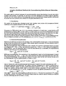
= (0; 1)2 with the right-hand side f and the Dirichlet boundary conditions according to the solution u(x; y) = (2 cosh 10)?1 (cosh(10x) + cosh(10y)) which has a boundary layer along the lines x = 1 and y = 1 (cf. Fig. 5.1). Problem 2. Equation (2.1) side f  0 and a hexagon  1 with  1right-hand p3  the p3 

with corners (1; 0),  2 ; 2 ,  2 ; ? 2 . The coecients are chosen according to b  0 and a(x; y) being piecewise constant with the values 1 and 100 on alternate triangles of the initial triangulation (cf. Fig. 5.2). The solution given by u(x; y) = a?1y(3x2 ? y) is continuous with a jump discontinuity of the rst derivatives at the interfaces. Starting from the initial coarse triangulations depicted in Figures 5.1 and 5.2, on each re nement level l the discretized problems are solved by preconditioned cg-iterations with a BPX-type preconditioner as described in Section 3. The iteration on level l + 1 is stopped when the estimated iteration error "l+1 is less then "2l+1   2l NNl+1l , with the safety factor  = 1:E ? 2, l denotes the estimated error on level l, the number of nodes on level l and l +1 are given by 23

Nl and Nl+1, respectively. Denoting by (~jl; u~l; ~l ) the resulting approximation and by u~^l the nonconforming extension of ~l , for the local re nement of Tl the elementwise error contributions 2K = ku~l ? u~^lk20;K , K 2 Tl, and the weighted P 2 ? 1 2 mean value  = j j K2Tl K are computed. Then, an element K 2 Tl is marked for re nement if jK j?12K  2 where  is a safety factor which is chosen as  = 0:95. The interpolated values of the level l approximation are used as startiterates on the next re nement level. For the global re nement process we use 2j j   tol ku~lk20; as stopping criteria, where  is a safety factor which is chosen as  = 0:95 and tol is the required accuracy, tol = 2:E ? 3.

Level 0, N = 8 Level 6, N = 5197 Figure 5.1: Initial triangulation T0 and nal triangulation T6 (Problem 1)

Level 0, N = 12 Level 5, N = 3641 Figure 5.2: Initial triangulation T0 and nal triangulation T5 (Problem 2) 24

estimated error/true error

Figures 5.1 and 5.2 represent the initial triangulations T0 and the nal triangulations T6 and T5 for Problems 1 and 2, respectively. For Problem 1 we observe a pronounced re nement in the boundary layer (cf. Fig. 5.1). For Problem 2 there is a signi cant re nement in the areas where the diusion coecient is large with a sharp resolution of the interfaces between the areas of large and small diusion coecient (cf. Fig. 5.2). 1.8 Boundary layer Discontinuous coefficients

1.7 1.6 1.5 1.4 1.3 1.2 1.1 1 10

100 1000 Number of nodes

10000

Figure 5.3: Error Estimation for Problem 1 and 2 Number of cg-iterations

50 45

Boundary layer Discontinuous coefficients

40 35 30 25 20 15 10 5 0 0

10000

20000 30000 40000 Number of nodes

50000

Figure 5.4: Preconditioner for Problem 1 and 2 The behaviour of the a posteriori L2-error estimator is illustrated in Figure 5.3 where the ratio of the estimated error and the true error is shown as a function of the total number of nodes. The straight and the dashed lines refer to Problem 1 (boundary layer) and Problem 2 (discontinuous coecients), 25

respectively. In both cases we observe a slight overestimation at the very beginning of the re nement process, but the estimated error rapidly approaches the true error with increasing re nement level. Finally, the performance of the preconditioner is depicted in Figure 5.4 displaying the number of preconditioned cg-iterations as a function of the total number of nodal points. Note that for an adequate representation of the performance we use zero as initial iterates on each re nement level and iterate until the relative iteration error is less than " = 1:E ? 6. In both cases, we observe an increase of the number of iterations at the beginning of the re nement process until we get into the asymptotic regime where the numerical results con rm the theoretically predicted O(1) behaviour.

References

[1] D.N. Arnold and F. Brezzi, Mixed and nonconforming2 nite element methods: implementation, post{processing and error estimates. M AN Math. Modelling Numer. Anal. 19, 7-35 (1985) [2] I. Babuska and W.C. Rheinboldt, Error estimates for adaptive nite element computations. SIAM J. Numer. Anal. 15, 736-754 (1978) [3] I. Babuska and W.C. Rheinboldt, A posteriori error estimates for the nite element method. Int. J. Numer. Methods Eng. 12, 1597-1615 (1978) [4] Bachmann, Adaptive Mehrgitterverfahren zur Losung der stationaren Halbleitergleichungen. Dissertation, Universitat Zurich (1993) [5] R.E. Bank, PLTMG - A Software Package for Solving Elliptic Partial Dierential Equations. User's Guide 6.0. SIAM, Philadelphia, 1990 [6] R.E. Bank, A.H. Sherman and A. Weiser, Re nement algorithm and data structures for regular local mesh re nement. In: Scienti c Computing, R. Stepleman et al. (eds.), p. 3-17, IMACS North{Holland, Amsterdam, 1983 [7] R.E. Bank and A. Weiser, Some a posteriori error estimators for elliptic partial differential equations. Math. Comp. 44, 283-301 (1985) [8] R.E. Bank, B. Welfert and H. Yserentant, A class of iterative methods for solving saddle point problems. Numer. Math. 56, 645-666 (1990) [9] F. Bornemann, B. Erdmann and Kornhuber, A posteriori error estimates for elliptic problems in two and three space dimensions. Konrad-Zuse-Zentrum fur Informationstechnik Berlin. Preprint SC 93-29, 1993 [10] F. Bornemann and H. Yserentant, A basic norm equivalence for the theory of multilevel methods. Numer. Math. 64, 445-476 (1993) [11] J.H. Bramble, J.E. Pasciak, J. Xu, Parallel multilevel preconditioners. Math. Comp. 55, 1-22 (1990) [12] F. Brezzi and M. Fortin, Mixed and Hybrid Finite Element Methods. Springer, Berlin{ Heidelberg{New York, 1991 [13] F. Brezzi, L.D. Marini and P. Pietra, Two dimensional exponential tting and application to drift-diusion models. SIAM J. Numer. Anal. 26, 1347-1355 (1989)

26

[14] F. Coulomb, Domain decomposition and mixed nite elements for the neutron diusion equation. In: Proc. 2nd Int. Symp. on Domain Decomposition Methods, T.F. Chan et al. (eds.), p. 295-313, SIAM, Philadelphia, 1989 [15] L.C. Cowsar, Domain decomposition methods for nonconforming nite element spaces of Lagrange-type. Rice University, Houston. Preprint TR 93-11, 1993 [16] W. Dahmen and A. Kunoth, Multilevel preconditioning. Numer. Math. 63, 315-344 (1992) [17] P. Deu hard, P. Leinen and H. Yserentant, Concepts of an adaptive hierarchical nite element code. IMPACT Comput. Sci. Engrg. 1, 3-35 (1989) [18] M. Dryja and O.B. Widlund, Towards a uni ed theory of domain decomposition alogrithms for elliptic problems. In: Proc. 3rd Int. Symp. on Domain Decomposition Methods for Partial Dierential Equations, T.F. Chan et al. (eds.), p. 3-21, SIAM, Philadelphia, 1990 [19] B. Erdmann, J. Lang and R. Roitzsch, KASKADE Manual, Version 2.0. Konrad-ZuseZentrum fur Informationstechnik Berlin. Technical Report TR 93-5, 1993 [20] B. Erdmann, R. Roitzsch and F. Bornemann, KASKADE Numerical experiments. Konrad-Zuse-Zentrum fur Informationstechnik Berlin. Technical Report TR 91-1, 1991 [21] R.E. Ewing, R.D. Lazarov, T.F. Russell and P.S. Vassilevski, Local re nement via domain decomposition techniques for mixed nite element methods with rectangular Raviart-Thomas elements. In: Proc. 3rd Int. Symp. on Domain Decomposition Methods for Partial Dierential Equations, T.F. Chan et al. (eds.), p. 98-114, SIAM, Philadelphia, 1990 [22] R.E. Ewing, T.F. Russell and M.F. Wheeler, Convergence analysis of an approximation of miscible displacement in porous media by mixed nite elements and a modi ed method of characteristics. Comput. Math. Appl. Mech. Eng. 47, 73-92 (1984) [23] R.E. Ewing and J. Wang, The Schwarz algorithm and multilevel decomposition iterative techniques for mixed nite element methods. In: Proc. 5th Int. Symp. on Domain Decomposition Methods for Partial Dierential Equations, D.F. Keyes et al. (eds.), p. 48-55, SIAM, Philadelphia, 1992 [24] R.E. Ewing and J. Wang, Analysis of multilevel decomposition iterative methods for mixed nite element methods. M 2 AN Math. Modelling and Numer. Anal. 28, 377-398 (1994) [25] R.E. Ewing 2and J. Wang, Analysis of the Schwarz algorithm for mixed nite element methods. M AN Math. Modelling and Numer. Anal. 26, 739-756 (1992) [26] B. Fraeijs de Veubeke, Displacement and equilibrium models in the nite element method. In: Stress Analysis, C. Zienkiewicz and G. Holister (eds.), John Wiley and Sons, New York, 1965 [27] R. Hiptmair and R. H. W. Hoppe, Mixed nite element discretization of continuity equations arising in semiconductor device simulation. In: Proc. Conf. Math. Modelling and Simulation of Electrical Circuits and Devices, R.E. Bank et al. (eds.), p. 197-217 Birkhauser, Basel, 1994 [28] R.H.W. Hoppe and A. Schmied, Adaptive mixed nite elements methods using uxbased a posteriori error estimators. In preparation. [29] R.H.W. Hoppe and B. Wohlmuth, Element-oriented and edge-oriented local error estimators for nonconforming nite elements methods. Submitted to M 2 AN Math. Modelling and Numer. Anal. [30] R.H.W. Hoppe and B. Wohlmuth, Adaptive multilevel iterative techniques for nonconforming nite elements discretizations. In preparation.

27

[31] C. Johnson, Numerical Solutions of Partial Dierential Equations by the Finite Element Method. Cambridge University Press, Cambridge, 1987 [32] T.P. Mathew, Schwarz alternating and iterative re nement methods for mixed formulations of elliptic problems. Part I: Algorithms and numerical results. Numer. Math. 65, 445-468 (1993) [33] T.P. Mathew, Schwarz alternating and iterative re nement methods for mixed formulations of elliptic problems. Part II: Convergence theory. Numer. Math. 65, 469-492 (1993) [34] S.V. Nepomnyaschikh, Fictitious components and subdomain alternating methods. Sov. J. Numer. Anal. Math. Modelling 5, 53-68 (1990) [35] S.V. Nepomnyaschikh, Decomposition and ctitious domain methods for elliptic boundary value problems. In: Proc. 5th Int. Symp. on Domain Decomposition Methods for Partial Dierential Equation, D.F. Keyes et al. (eds.), p. 62-72, SIAM, Philadelphia, 1992 [36] R.R.P. van Nooyen, Some aspects of mixed nite elements methods for semiconductor simulation. Ph.D. Thesis, University of Amsterdam, 1992 [37] P. Oswald, Two remarks on multilevel preconditioners. Forsch.-Erg. FSU Jena, Math. /91/1, 1991 [38] P. Oswald, On a hierarchical basis multilevel method with nonconforming P1 elements. Numer. Math. 62, 189-212 (1992) [39] P. Oswald, On discrete norm estimates related to multilevel preconditioner in the nite elements methods. In: Constructive Theory of functions, K.G. Ivanov et al. (eds.), p. 203-214, Bulg. Acad. Sci, So a, 1992 [40] P. Oswald, On a BPX-preconditioner for P1 elements. Computing 51, 125-133 (1993) [41] P. Oswald, Multilevel nite element approximation: Theory and Application. To appear: Teubner-Skripten zur Numerik, Teubner, Stuttgart [42] A. Reusken, Multigrid applied to mixed nite elements schemes for current continuity equations. Preprint Technical University Einhoven (1990) [43] T. Rusten and R. Winther, A preconditioned iterative method for saddle point problems. SIAM J. Matrix Anal. Appl. 13, 887-904 (1992) [44] C. Srinivas, B. Rumasuany and M.F. Wheeler, Mixed nite elements methods for ow through unstructed porous media. In: Computational Methods in Water Resarces IX Vol. 1, T.F. Russel, C.A. Brebbia, R.E. Ewing, W.G. Gray and G.F. Pinder (eds.), p. 239-246, Denver 1992 [45] B. Szabo and I. Babuska, Finite Element Analysis. John Wiley & Sons, New York, 1991 [46] P.S. Vassilevski and J. Wang, Multilevel iterative methods for mixed nite elements discretizations of elliptic problems. Numer. Math. 63, 503-520 (1992) [47] R. Verfurth, A posteriori error estimation and adaptive mesh-re nement techniques. To appear in J. Comp. Appl. Math. [48] R. Verfurth, A review of a posteriori error estimation and adaptive mesh-re nement techniques. Manuscript, 1993 [49] B. Wohlmuth and R.H.W. Hoppe, Multilevel approaches to nonconforming nite elements discretizations of linear second order elliptic boundary value problems. To appear in Journal of Computation and Information [50] J. Xu, Iterative methods by space decomposition and subspace correction. SIAM Rev. 34, 581-613 (1992)

28

[51] H. Yserentant, Hierarchical bases in the numerical solution of parabolic problems. In: Proc. Meet. Large Scale Scienti c Computing, P. Deu hard et al. (eds.), p. 22-36, Birkhauser, Basel, 1987 [52] H. Yserentant, Old and new convergence proofs for multigrid methods. Acta Numerica 1, 285-326 (1993) [53] X. Zhang, Multilevel Schwarz methods. Numer. Math. 63, 521-539 (1992) [54] O.C. Zienkiewicz and R.L. Taylor, The Finite Element Method, Vol. 1. Mc Graw-Hill, London, 1989

29