Sep 13, 2001 - arXiv:hep-lat/0109005v1 13 Sep 2001. 1. MS-TP-01-3, IFUP-TH 2001/26. Adaptive Optimization of Wave Functions for Lattice Field Models.
1
MS-TP-01-3, IFUP-TH 2001/26
arXiv:hep-lat/0109005v1 13 Sep 2001
Adaptive Optimization of Wave Functions for Lattice Field Models Matteo Beccariaa,b , Massimo Campostrinia,c Alessandra Feod a
Istituto Nazionale di Fisica Nucleare Dipartimento di Fisica, Universit`a di Lecce c Dipartimento di Fisica, Universit`a di Pisa d Institut f¨ ur Theoretische Physik, Westf¨alische Wilhelms-Universit¨ at, M¨ unster, Germany. b
Abstract The accuracy of Green Function Monte Carlo (GFMC) simulations can be greatly improved by a clever choice of the approximate ground state wave function that controls configuration sampling. This trial wave function typically depends on many free parameters whose fixing is a non trivial task. Here, we discuss a general purpose adaptive algorithm for their non-linear optimization. As a non trivial application we test the method on the two dimensional Wess-Zumino model, a relativistically invariant supersymmetric field theory with interacting bosonic and fermionic degrees of freedom.
1
Introduction
The traditional algorithms for numerical simulations of Lattice Field Theories are based on the Lagrangian formulation [1] that follows Feynman’s idea of representing quantum amplitudes in terms of sums over classical paths. An interesting alternative is the Hamiltonian framework of KogutSusskind [2] focusing on the Hamiltonian as the generator of the temporal evolution. To improve numerical efficiency in the evaluation of physical
2
M. Beccaria, M. Campostrini, A. Feo
observables, analytical approximations of the ground state wave function can be successfully exploited. This well known procedure is called Importance Sampling [3] and its key problem is to determine the optimal trial wave function (TWF) within a given class depending parametrically on a set of free parameters. In this contribution, we review a recently proposed algorithm that solves this problem. It is built upon a standard Green Function Monte Carlo (GFMC) simulation algorithm and is based on a non trivial feedback between Monte Carlo evolution and TWF modifications. To discuss the method, we present some novel results concerning the calculation of the ground state energy of the supersymmetric N = 1 WessZumino model in 1 + 1 dimensions.
2
Review of Green Function Monte Carlo
GFMC algorithms can be regarded as numerical implementations of the Feynman-Kac formula [4]. In the simple case of Quantum Mechanics, this formula claims that, given the potential V (q) and an initial wave function ψ0 (q), the function �
ψ(q, t) = E ψ0 (q + Wt ) exp −
Z
t 0
�
V (q + Ws )ds ,
(where Wt is the Wiener process) solves the Euclidean Schr¨odinger equation 1 ∂t ψ(q, t) = ∆ψ(q, t) − V (q)ψ(q, t) 2 with initial data ψ(q, 0) = ψ0 (q). A translation of this formula into a numerical algorithm is straightforward and quantum expectation values over the ground state can be expressed as statistical averages over an ensemble of weighted walkers [5]. As is well known, the weight variance of the ensemble members must be controlled in some way. Here we adopt the Stochastic Reconfiguration algorithm with fixed population size [6]. The finite population size bias as well as walker correlations vanish with increasing number of walkers. Weight fluctuations are closely related to the noise of measurements and are due to the fact that V is not constant along walker paths. To
GFMC Calculation of Wave Functions for Quantum Field Models
3
significantly improve accuracy one needs to reduce these fluctuations. Importance Sampling is a common strategy to achieve such a noise reduction: the original Hamiltonian H = 12 p2 + V (q) is transformed into f = eF He−F = 1 p2 + ip · ∇F + Ve , H 2
1 1 Ve = V − ∆F − (∇F )2 . 2 2
f is not canonical, but still allows simulations with minor modifications H with respect to the F ≡ 0 case [5]. The diffusion of the walkers is driven by a drift term proportional to ∇F while the potential V (q) is replaced by a new potential Ve that depends on the trial wave function through F . Roughly speaking, a true improvement is reached when Ve is more constant than V along random paths in some way we are going to discuss later on.
3
Adaptive Optimization of the Wave Function
In this Section, we show how the trial wave function F can be optimized dynamically within Monte Carlo evolution. To this aim, we consider a parametric TWF exp F (q, a) depending on the state degrees of freedom q and on a set of free parameters a. After N Monte Carlo steps, a simulation with a population of K walkers furnishes a biased estimator Eˆ0 (N, K, a) of the ground state energy E0 that we shall take as a representative observable. Eˆ0 is thus a random variable such that ˆ0 (N, K, a)i = E0 + hE and
c1 (a) + o(K −α ), Kα
α > 0,
c2 (K, a) , Var Eˆ0 (N, K, a) ∼ √ N
where h·i is the average with respect to Monte Carlo realizations. In the K → ∞ limit, hEˆ0 i is therefore exact and independent on a. The constant c2 (K, a) is related to the fluctuations of the effective potential Ve and is strongly dependent on a. The problem of finding the optimal F can be translated in the minimization of c2 (K, a) with respect to a.
4
M. Beccaria, M. Campostrini, A. Feo
The algorithm we propose [5] performs this task by interlacing a Stochastic Gradient steepest descent with the Monte Carlo evolution of the walkers ensemble. At each Monte Carlo step, we update an → an+1 according to the simple law an+1 = an − ηn ∇a VarEn Ve
where En is the ensemble at step n and {η} is a suitable sequence, asymptotically vanishing. A non-linear feedback is thus established between the TWF and the evolution of the walkers. The convergence of the method can not be easily investigated by analytical methods and explicit numerical simulations are required to understand the robustness of the algorithm. In reference [5], examples of applications of the method with purely bosonic or fermionic degrees of freedom can be found. In the next Section, we shall address a model with both kinds of fields linked together by an exact lattice supersymmetry.
4
The N = 1 Wess-Zumino Model in 1+1 Dimensions and Supersymmetry Breaking
The model we consider is a lattice version of the N = 1 Wess-Zumino model previously studied in [7]. On each site of a spatial lattice with L sites, we define a real scalar field {ϕn } together with its conjugate momentum {pn } such that [pn , ϕm ] = −iδn,m . The associated fermion is a Majorana fermion {ψa,n } with a = 1, 2 and {ψa,n , ψb,m } = δa,b δn,m , † ψa,n = ψa,n . The fermionic charge Q=
L � X
n=1
�
�
�
ϕn+1 − ϕn−1 pn ψ1,n − + V (ϕn ) ψ2,n , 2
with arbitrary real prepotential V (ϕ), can be used to define a semi-positive definite Hamiltonian H = Q2 . Its positive eigenstates are automatically paired in doublets connected by Q; only a Q-symmetric ground state with zero energy can be unpaired. H describes an interacting model, symmetric with respect to Q; its ground state breaks the symmetry if and only if its energy is positive. We stress that spontaneous supersymmetry breaking can occur even for finite L, because tunneling among degenerate vacua connected by Q is forbidden by fermion number conservation.
GFMC Calculation of Wave Functions for Quantum Field Models
5
We can replace the two Majorana fermion operators with a single Dirac operator satisfying {χn , χm } = 0, {χn , χ†m } = δn,m [7]. The Hamiltonian takes then the form H =
X n
(
�
1 2 1 ϕn+1 − ϕn−1 p + + V (ϕn ) 2 n 2 2 �
�2
+
1 1 − (χ†n χn+1 + h.c.) + (−1)n V ′ (ϕn ) χ†n χn − 2 2 † = HB (p, ϕ) + HF (χ, χ , ϕ)
��
and describes canonical bosonic and fermionic fields with standard kinetic energies and a Yukawa coupling. The theoretical problem that we want to address is dynamical breaking of supersymmetry in the above kind of models. At tree level, supersymmetry breaking occurs if and only if V (ϕ) has no zeroes. In 1 + 1 dimensions, this picture is known to be unstable with respect to radiative corrections as shown by the analysis of the one-loop effective potential of the scalar field ϕ. From the non-perturbative point of view, the ground state energy E0 is the crucial quantity because it vanishes if and only if we are in the symmetric phase. The choice of a Hamiltonian Monte Carlo algorithm is then natural since E0 is the simplest observable that can be measured with such a technique. We study two specific examples: the cubic prepotential V (ϕ) = ϕ3 , where unbroken supersymmetry is expected, and the family of quadratic prepotentials V (ϕ) = λ0 +ϕ2 . In the latter case, at tree level supersymmetry is broken for λ0 > 0. Perturbative calculations and previous numerical results [7] suggest that this conclusion does not hold at the quantum level and provide evidence that supersymmetry is broken in the lattice model for λ0 greater than some negative λ∗0 < 0 and is recovered for λ0 ≤ λ∗0 . On the other hand, the strong-coupling limit suggests E0 > 0 for all λ0 , decreasing exponentially for λ0 → −∞ [8]; moreover, one can show that, at fixed finite L, E0 is an analytical function of λ0 ; this would imply that a symmetric phase is only possible in the L → ∞ limit. 4.1
Simulation Algorithm: Brief Description
The Monte Carlo evolution in GFMC algorithms approximates the Hamiltonian evolution semigroup {e−tH }t≥0 . The bosonic and fermionic degrees
6
M. Beccaria, M. Campostrini, A. Feo
of freedom can be split by writing e−βH = e−1/2
βHB −βHF −1/2 βHB
e
e
+ O(β 3 ),
and the β → 0 extrapolation is numerically computed at the end. We implement the evolution associated to HB to second order in β [9] and the evolution associated to HF exactly [10]. About the choice of the trial wave function, we propose the factorized form † |ΨT0 i = eSB (ϕ)+SF (ϕ,χ,χ ) |Ψ0 iB ⊗ |Ψ0 iF ,
where |Ψ0 iB ⊗ |Ψ0 iF is the ground state for the free model and SB =
dB XX
αkB ϕkn ,
n k=1
SF =
X n
n
(−1)
�
χ†n χn
1 − 2
� X dF
αkF ϕkn .
k=1
The degrees dB and dF must be chosen carefully to achieve convergence of the adaptive determination of {αB , αF }. In the regime of weak coupling perturbation theory, the choice of periodic boundary conditions does not break supersymmetry when L mod 4 = 0. Under this condition, there is an even number of fermions, L/2, in the ground state. A sign-problem then arises due to boundary crossings since they involve an odd number of fermion exchanges. To avoid such a difficulty, we shall adopt open boundary conditions. With this choice, L needs just to be even to assure a supersymmetric weak coupling ground state. In the following, we shall restrict ourselves to the case L mod 4 = 2 and to the sector with L/2 fermions that contains a non-degenerate ground state, with zero energy at all orders in a weak coupling expansion. 4.2
Numerical Results
We choose dB = dF = 4; due to the symmetries of the model with quadratic V (ϕ) = λ0 + ϕ2 , we impose parity constraints on the trial wave function, setting α1B , α3B , α2F , α4F to zero (α1B , α3B , α1F , α3F in the cubic case), and and determine by the adaptive algorithm the remaining four free parameters. We work on a lattice with 10 spatial sites and vary both K and λ0 . In principle, we also extrapolate any result to the β → 0 limit. However, the results we present are all obtained with a fixed value β = 0.01 since we checked that a reduction of this parameter by a factor 2 does not change appreciably the results.
GFMC Calculation of Wave Functions for Quantum Field Models
7
1.0
Trial Wave Function Parameters
0.8
α
F
0.6
1
0.4
0.2
0.0
α
−0.2
α
F 3
Β 4
Β
−0.4
α 0
1
2
2 3
5
4
5
Monte Carlo iteration ( x 10 )
Figure 1: Adaptive Optimization of the four coefficients appearing in the trial wave function for the quadratic model. The constant λ0 is 0.0 and the ensemble size is K = 100.
Beginning with a small ensemble of K = 100 walkers, we determine adaptively the four coefficients {α2B , α4B , α1F , α3F } starting from zero values. A typical run is shown in Fig. (1). For larger K, we start from the values of α obtained in a run at the nearest smaller K. A summary plot of {α2B , α4B , α1F , α3F } as functions of K and λ0 is shown in Fig. (2). With the optimized TWF parameters, we determine the energy contributions coming from the bosonic and fermionic sectors separately. The sum of the two is the total ground state energy E0 . Apart from the dependence on β, E0 is a function of three parameters E0 = E0 (λ0 , L, K), where we understand our choice of TWF and also optimization of its free parameters. The dependence on K is totally artificial and we are interested in E0 (λ0 , L, ∞). The dependence on L enters the study of the continuum limit of the model. However, here we simply want to test the method and work at fixed L = 10. For the quadratic case, we show in Fig. (3) the behavior of E0 (λ0 , L, K) as a function of K at several values of λ0 . For λ0 > −0.5 the K dependence is very mild and one can confirm the claim that a positive E0 (λ0 , L, ∞) >
8
M. Beccaria, M. Campostrini, A. Feo
0.40
−0.065
α
0.20
−0.070
K=100 K=200 K=500 K=1000 K=1700 K=3000 K=5000
0.00 −0.20 −0.40 −2.5
Β 2
−2.0
−1.5
1.10
α
Β 4
−0.075 −0.080
−1.0 λ0
−0.5
1.00
−0.085 0.5 −2.5
−2.0
−1.5
−0.04
α
1.05
0.0
F 1
−0.06
α
−1.0 λ0
−0.5
0.0
0.5
−1.0 λ0
−0.5
0.0
0.5
F 3
0.95 0.90
−0.08
0.85 0.80
−0.10
0.75 0.70 −2.5
−2.0
−1.5
−1.0 λ0
−0.5
0.0
0.5
−0.12 −2.5
−2.0
−1.5
Figure 2: Summary plots of the four trial wave function parameters as a function of λ0 and K.
0 is obtained at K → ∞. Instead, for λ0 < −0.5, there is a certain dependence on K and an extrapolation toward K → ∞ must be performed to determine the asymptotic limit. Fig. (4) shows the results of such an extrapolation. For λ0 ≥ −1.25, we can exclude a zero E0 (λ0 , L, ∞); for λ0 ≤ −1.5 our data are compatible with zero. On the other hand, for the cubic potential the dependence of E0 on K is relatively mild; in Fig. (5) we show that E0 is compatible with 0 for K ≥ 500, in full agreement with the expectation of unbroken supersymmetry. It should be noticed that bosonic and fermionic contributions to E0 are of the order of 10, and the two are canceling to a precision of 10−4 . The conclusion we can draw from the above numerical data is that the presented algorithm behaves in a completely satisfactory way in the analysis of the N = 1 Wess-Zumino model, at least for what concerns the determination of the ground state energy. In the L = 10 lattice
GFMC Calculation of Wave Functions for Quantum Field Models
9
1
10
0
Total Energy
10
−1
10
K = 100 K = 200 K = 500 K = 1000 K = 1700 K = 3000 K = 5000 K = 10000
−2
10
−3
10
−1.8 −1.6 −1.4 −1.2 −1.0 −0.8 −0.6 −0.4 −0.2 0.0 λ0
0.2
Figure 3: Total energy in log scale as a function of λ0 and K.
quadratic model supersymmetry is broken with no doubts for values of λ0 down to about λ0 ≃ −1.25. Below this value, E0 is compatible with zero at the statistical level we work. We remark that around λ0 ≃ −0.75 the coefficient α2B changes sign, modifying the shape of the TWF and allowing for local minima in its ϕ-dependent part SB (ϕ) at non zero fields; we interpret this fact as an interesting signal that some transition is occurring and emphasize the important role that trial wave functions play. On the other hand, for the cubic model the evidence for unbroken supersymmetry is quite convincing. Unbroken supersymmetry implies a number of non-trivial Ward identities; we monitored several of these, obtaining a pattern of supersymmetry
10
M. Beccaria, M. Campostrini, A. Feo
0.14 0.12
Total Energy
0.10
λ0 = −0.75 λ0 = −1.00 λ0 = −1.25 λ0 = −1.50 λ0 = −2.00
0.08 0.06 0.04 0.02 0.00 −0.02
−4
10
−3
10 1/K
−2
10
Figure 4: Extrapolation of the total energy in the K → ∞ limit. The various curves are drawn for several values of λ0 . Data points corresponds to K = 100, 200, 500, 1000, 1700, 3000, 5000, and 10000.
breaking perfectly consistent with the one obtained from E0 , although with lower numerical precision [11].
5
Conclusions
The Hamiltonian approach is a powerful method for Monte Carlo analysis of field models. It is well founded and general purpose, but the control of systematic errors is fundamental. A good trial wave function can improve strongly the quality of numerical results and the convergence rate
−1
10
GFMC Calculation of Wave Functions for Quantum Field Models 11
0.008
Total Energy
0.006
0.004
0.002
0.000
−0.002
10
−3
10
−2
1/K Figure 5: For the cubic potential, extrapolation of the total energy in the K → ∞ limit. Data points corresponds to K = 100, 200, 500, 1000, and 2000.
of simulations. The trial wave function is an approximation to the exact ground state. As such, it contains important physical informations about the model under study. Optimization of (many-parameter) wave functions is thus not only motivated by computational needs only. It affords and checks analytical insights about the actual ground state. Moreover, as we have shown, for certain models in 1 + 1 dimensions, the Hamiltonian formalism appears to be the natural framework for lattice fermions. The treatment of bosons and fermions is nicely symmetric and the non-local determinants required in Lagrangian simulations are not required at all. The possibility of preserving exactly a 1-dimensional
10
−1
12
M. Beccaria, M. Campostrini, A. Feo
supersymmetry algebra is also very appealing.
References [1] K. Wilson, Phys. Rev. D10 (1974), 2445. [2] J. Kogut, L. I. Susskind, Phys. Rev. D11 (1975), 395; J. Kogut, Rev. Mod. Phys. 51 (1979), 659. [3] D. M. Ceperley, M. H. Kalos, “Monte Carlo Methods in Statistical Physics”, edited by K. Binder, Springer-Verlag, Heidelberg (1992). [4] B. Simon, “Functional integration and quantum physics”, Academic Press, Inc., New York (1979). [5] M. Beccaria, Europhys. Journal C13 (2000), 357; Phys. Rev. D61 (2000), 114503; Phys. Rev. D62 (2000), 34510. [6] M. C. Buonaura and S. Sorella, Phys. Rev. B57 (1998), 11446. [7] J. Ranft, A. Schiller, Phys. Lett. B138 (1984), 166; for a theoretical discussion see also S. Elitzur, E. Rabinovici, A. Schwimmer, Phys. Lett. B119 (1982), 165. A similar approach to Wess-Zumino models with N = 2 supersymmetry is discussed in S. Elitzur, A. Schwimmer, Nucl. Phys. B226 (1983), 109 and numerical investigations are reported in A. Schiller, J. Ranft, J. Phys. G12 (1986), 935. [8] E. Witten, Nucl. Phys. B188 (1981), 513; Nucl. Phys. B202 (1982), 253. [9] S. A. Chin, Proc. of 1988 Symp. on Lattice Field Theory, Batavia, IL, Sept. 22-25 (1988), Nucl. Phys. (Proc. Suppl.) 9 (1989) 498. [10] M. Beccaria, A. Moro, Phys. Rev. D64 (2001), 077502. [11] M. Beccaria, M. Campostrini, A. Feo, proceedings of the XIX International Symposium on Lattice Field Theory, LATTICE2001, Berlin, August 19-24 (2001). To appear on Nucl. Phys. (Proc. Suppl.).