Adaptive Predictor for Lossless Image Compression - Springer Link

Computing 62, 339–354 (1999) c Springer-Verlag 1999

Printed in Austria

Adaptive Predictor for Lossless Image Compression V. Hlav´acˇ and J. Fojt´ık, Prague Received June 29, 1998; revised November 2, 1998 Abstract A new method for lossless image compression of grey-level images is proposed. The image is treated as a set of stacked bit planes. The compressed version of the image is represented by residuals of a non-linear local predictor spanning the current bit plane as well as a few neighbouring ones. Predictor configurations are grouped in pairs differing in one bit of the representative point only. The frequency of predictor configurations is obtained from the input image. The predictor adapts automatically to the image, it is able to estimate the influence of neighbouring cells and thus copes even with complicated structure or fine texture. The residuals between the original and the predicted image are those that correspond to the less frequent predictor configurations. Efficiently coded residuals constitute the output image. To our knowledge, the performance of the proposed compression algorithm is comparable to the current state of the art. Especially good results were obtained for binary images, grey-level cartoons and man-made drawings. AMS Subject Classifications: 68T10. Key Words: Image compression, non-linear predictor.

1. Introduction Data compression can be viewed as a process producing a model of the input data together with associated residuals. An improved data model yields better compression results. Redundant information in generic raster images is due to high correlation between neighbouring cells.1 In other words, the local structure and similarity are the main source of redundancy in generic imagery. The proposed image compression method examines the neighbourhood of the current cell using an adaptive probe, creates a non-linear predictor for the current cell value, and stores residuals of the predictor in the resulting compressed image. In the compression phase, an image is systematically traversed using an adaptive probe and, for the current cell, a non-linear predictor is created by examining the local neighbourhood. The estimated value is compared to the actual value of the 1 The term cell is used instead of pixel common for 2D images as it copes with higher dimensions too.

340

V. Hlav´acˇ and J. Fojt´ık

cell. Where there is a discrepancy between the estimated and the actual value the residual (binary value one) is stored in the position of the current cell. If the predictor provides a good estimate, a precise match will be found for the majority of the cells and the resulting compressed image will be small. The description of the predictor and the positions of the residuals in the image are stored together in the output file. Three predictors with increasing complexity are described in this paper, i.e. (i) for binary images, (ii) for grey-level images, (iii) adaptive predictor for grey-level image. The reduced data is optimally coded, and together with the predictor description, the compressed image is created. The paper is organised as follows. Section 2 lists the current most efficient lossless compression methods and these are later used for comparison with the proposed methods. Section 3 explains the basic predictor as a set of probe pairs that differ in one bit only. Section 5 generalises the predictor for the grey-level image that is treated as stacked bit planes. Section 6 further improves the predictor by allowing it to adapt to the actual image data. Section 7 proposes an efficient way to encode the sparse matrix of predictor residuals. In Section 8 we present experimental results. In the last section we draw conclusions. A preliminary version of the paper was published in [4]. 2. Related Works There are several lossless compression methods used for 1D streams of data as text or executable programs. The ZIP or LZW are examples of commonly used packages. They are known and we do not describe them here. Let us begin with describing some methods similar to ours developed for 2D compression. Lossless compression techniques are usually divided into two generations. The methods in the first generation use quite simple algorithms. Let us just mention three representatives here. The IBM Q80 coder (lossless JPEG) [1] is obsolete and outperformed by the conceptually similar Portable Network Graphics (PNG). PNG [10] consists of two steps. In the first step, the difference image 1x (x, y) = f (x − 1, y) − f (x, y) is computed and a matrix which contains only differences is created. In the second step, this matrix is encoded using the LZW method. Both parts may be connected by a pipe and these can run in parallel. The source code of the algorithm is freely available. The disadvantage is that the second step is not tuned to 2D image data. PNG is based on the assumption that the number of regions with limited 1st derivatives is smaller than the number of regions with higher 1st derivatives. The context of the images is richer.

Adaptive Predictor for Lossless Image Compression

341

Paper [2] discusses several simple compression methods PVRG-JPEG proposed by the Portable Video Research Group at Stanford. Each method was tried on the images and the best method was selected for actual compression. The second generation lossless compression methods are usually divided into two subgroups: Region based. The image is divided into regions that have similar intensity or other properties. Regions are compressed separately and stored together with a description of the boundary of the region. The method Segment [8] belongs to this group. The regions are grown from seeds. The resulting compression ratios are very good. Data prediction based methods try to create an internal data model. Residuals of the model are stored. A method which is performing similarly to ours that has similar results is called Callic [11]. It calculates several features from the pixels in a small neighbourhood. The pixels in the predictor are chosen adaptively using information from image directional derivatives. The rounding transform from [6] uses circular-shaped hierarchical estimators. The compression ratio does not rank the method among the best. There is one more method which is relevant to ours. It treats the image as separate bit planes and is called the Logic coding method [5]. The method uses boolean logic for image compression. 3. Idea of Image Coding for Binary Image The initial idea comes from Schlesinger [9] who proposed a new representation scheme for binary images. Let us denote the method by Schl-2. Number 2 comes from two degrees of freedom (DOF). The Schl-2 method takes a binary image f as input. The support of the image is T ={(x, y) : 0 ≤ x ≤ M; 0 ≤ y ≤ N }, where M is the width of the image and N is the height. The image represents the mapping f (x, y) → {0, 1}. Without loss of generality, we assume that the leftmost column and the bottom line of the image have value zero, i.e. f (0, y) = f (x, 0) = 0.

p3

p4

p2

p1

Figure 1. 2 × 2 probe of the predictor

V. Hlav´acˇ and J. Fojt´ık

342

The Schl-2 method traverses the binary image f by the probe consisting of 2 × 2 cells. Its representative cell (x, y) is placed in the upper right corner of the probe. The value of the actual (estimated) cell is p4 = f (x, y). Let values of the probe placed in the particular position in the probe be denoted p1 = f (x, y − 1); p2 = f (x − 1, y − 1); p3 = f (x − 1, y); see Fig. 1.

p4 = 0

p4 = 1 1

2

3

4

5

6

7

8

Figure 2. Predictor used for binary image coding. All possible configurations are arranged into eight pairs differing in the upper right bit only. Highlighted configurations are treated as less frequent

Schlesinger designed the predictor (estimator, probe) e in the following way. All the 16 possible combinations of cells within the 2 × 2 probe are considered. Probes are arranged into two rows and eight columns in such a way that probes in the same column differ in the upper right bit only, see Fig. 2. A frequency analysis of the predictor configurations was performed on many different images with the aim of finding out which configuration in each pairs occurs more often. The more frequent configurations are highlighted in Fig. 2. The probes in column 5 will be discussed soon. The idea of this compression method is to store residuals of less frequent probes, i.e. bit one in the representative point of the probe. The arrangement of the probes allows us to reconstruct the image from a sparse matrix of stored residuals only. Schlesinger tested the predictor on many images and the more frequent probe of each pair was found through extensive experiments. In the compression phase, only the residuals between predicted and real values are stored. This typically yields a much sparser image. Actually, the probe configurations proposed by Schlesinger are suboptimal with respect to the relative frequencies of different configurations. Probes in Fig. 2, column 5 would have to be highlighted in opposite manner if the probe statistics had to be optimal. A substantial advantage of the suboptimal configurations independent of the image content is that standard set operations (intersection, union, negation) and binary morphology operations can be performed on the compressed images.

Adaptive Predictor for Lossless Image Compression

343

4. Compression of Binary Images Our compression method for binary images abbreviated as FH-2 takes a step forward compared to Schlesinger’s one. The probe frequency analysis is performed for each image. The result is then stored in a frequency table consisting of two rows and eight columns. A value in the table represents the number of occurrences of the corresponding probe in the image. The maxima in the frequency table point to optimal predictor configurations. These are marked. One bit is needed to distinguish between two probes in one column. Thus one byte describes all eight pairs of probes. This information will be added to the compressed image to store the predictor description. In the compression phase, the image is traversed in a bottom-up manner and from right to left. In each position of the image, a check is made to determine whether a more frequent or less frequent probe appeared. In the former case, the value 0 is written to the representative cell. Whereas, in the latter case, the value one is stored (corresponding to the residual of the predictor). The algorithm traverses the whole image and produces an image of residuals. This reduced image is typically much sparser than the input image due to the estimation abilities of the predictor. The decompression phase has at hand the description of the predictor (one byte) and the image of residuals. The left-most column and the bottom most row are known to be zero-valued. The probe starts at the bottom left corner with the values p1 , p2 , and p3 being known. These three values uniquely determine one of the eight columns of the predictor. The value of the stored residual distinguishes the correct probe in the pair. The decompressed value p4 is set accordingly and overwrites the residual in the position p4 . The probe traverses the image row-wise from left to right and from bottom to top, until the original image is restored. 5. Compression of Grey-Level Images The grey-level image can be treated as stacked bit planes. The predictor described in the previous section was generalised to cope with the current bit plane and the closest bit plane upwards. The predictor context encompassed by the volumetric probe has three degrees of freedom (DOF). Therefore we abbreviate the proposed compression algorithm FH-3. The arrangement of cells in the probe is shown in Fig. 3. The processed bit plane is the lower one. Its representative point, i.e. the predicted cell, is denoted by p8 and is highlighted. The idea of the compression remains the same as in the binary case. The frequency analysis of probe configurations is performed when passing through the image for the first time. The process is analog to the binary image case described in Section 3. Here 27 bits = 16 bytes are needed to store the frequency table of all possible configurations. The image of the processed bit-plane is reduced and

V. Hlav´acˇ and J. Fojt´ık

344

p3 p1

p4 p2 p8

p7 p6

p5

Upper bit plane

Current bit plane

Figure 3. F H − 3 predictor

residuals are stored in the same way as in the binary image case. This requires a second pass through the original image data. The result is a sparse matrix with a small number of residuals. Top bit plane p2

p1 p2

p3 p4

p3 p4

p7 p 8 p5 p 6

p7

p11 p12 p9 p 10

p5

p8

p6

p3 p4 p7 p 8 p5 p 6

p7 p 8 p5 p 6

p11 p12 p9 p 10

p11 p12 p9 p 10

p11 p12 p9 p 10

p11 p12 p9 p 10

Figure 4. Modified probes spanning several bit planes

The original image can be uniquely reconstructed using the residuals and the description of the predictor stored in the compressed image. The compression process as described above starts from the top bit plane using the FH-2 algorithm (since there is no available data above the top plane). Then the FH-3 algorithm is applied to remaining bit planes. More complicated probes spanning several bit planes can be also used, see Fig. 4. The rightmost probe is used for processing the top bit plane. The probe to the left is used for coding the bit plane below the top plane and so on. 6. Adaptive Compression The two previous predictors had a fixed number of probe cells (3 in the Schl-2 case and 7 in the FH-3 case) in a fixed arrangement. The desire is to exploit a more

Adaptive Predictor for Lossless Image Compression

345

complex image context in the predictor. The support set of the predictor can vary in more dimensions according to the context of the image. Such a predictor can encode more complicated structures in the image, e.g. some fine texture. The size of the predictor support is limited from a practical point of view by the size of the frequency table. The size of the frequency table grows exponentially and has 2k entries, where k is the number of cells of the predictor. The predicted representative cell of the probe is not counted. For example, for 20 cells, the frequency table size is 220 = 1Mbit. This would be too much. Of course, not all predictor cells contain the same amount of information. The trick we propose is to throw away some cells from a relatively large probe adaptively. This is done according to the content of the particular image. In the following, let us denote such an adaptive predictor by FH-Adapt in the sequel. The construction of predictor probes is similar to the procedure described earlier. They have more cells, e.g. 20, and could span n-DOF (degrees of freedom). In the case of an RGB colour image, there are 3-DOF in the intensity image corresponding to one of the colour components. The two other DOF are added by the context in the same bit-plane in other two colour components. Probes are again arranged in pairs that differ only in the value of the actual (estimated) cell. This facilitates a unique reconstruction of the original image in the decompression phase. The frequency analysis comes next. The result of the analysis is the frequency table with the size 2k+1 , where k is the number of support cells of the predictor. Note that there is no need for the representative cell to be in the set of k elements in the probe. The frequency table is usually rather big. The aim is to select the subset of i cells, i < k, containing most of the information. This results in a reduction of the length of the frequency table to 2i . The selection step does not need to pass through the original image another time and thus is independent of the size of the image. Predictor cells may be viewed as features in statistical pattern recognition task. The cells contribute to the estimate of the representative point of the probe. After the frequency analysis, it is known how often a particular predictor probe occurs in the image. Moreover, the cells can be ordered according to their importance for estimation of the representative cell. The proposed algorithm decouples the influences of individual cells from the frequency table. Let us explain the decoupling in the specific case of a binary image. The aim is to reduce the number of probe cells by one to k = 3. All configurations of the probe were shown in Fig. 2. Assume for a moment that we would like to decouple the influence of cell p3 (the top left corner of the probe). If this feature was omitted the probe pairs would merge as shown in Fig. 8. The frequency of the new probe configuration is the sum of the frequencies of its two constituting configurations, which differ only by the value of the removed cell.

V. Hlav´acˇ and J. Fojt´ık

346

An appropriate representation of the frequency table facilitates the use of very efficient bit operations. Recall that the representative cell has the highest index. Let the frequency table be stored in a vector q with 2k+1 elements. The first 2k elements of the vector q = (q0 , . . . , qk ) correspond to the frequencies of the top row of probe configurations. Let eall be the number of occurrences of the less frequent configurations of the probes. Furthermore, let b be an index to the first element of the second half of the frequency table, b = 2k , and c the index of the removed cell. The value eall is calculated as eall =

b−1 X

min(qi , qi+b ).

i=0

Let ec denote a measure of the estimativness of a cell with index c. ec = eall −

b−1 1X min (qi + qi⊕c , qi⊕b + qi⊕c⊕b ) . 2 i=0

The factor 12 in front of the sum comes from the fact that the value within the sum is considered twice. The estimativness ec expresses the increase in the number of residuals when the cell c is omitted. The operator ⊕ denotes logical eXclusive OR. The cell with the lowest estimativness ec is omitted from the probe. This algorithm can be applied iteratively and in each iteration the cell corresponding to the minimal value ec is thrown away. At last, we will define the termination criterion for removal of cells. The number of residuals eall increases monotonically if we throw away cells one by one. The number of entries in the frequency table decreases monotonically and thus its length decreases. We are trying to find the extremum of the difference between these two functions. If the increase of the length of the coded residuals (given by the value ec ) is bigger than the decrease of the table length or the table is empty then the algorithm terminates. 7. Encoding Residuals To achieve high compression ratio the matrix of residuals should be efficiently coded. Consider Fig. 5 where a simple example of residuals is shown. The idea is to code residuals along line scans using distances between residuals. The counting starts from an hypothetical starting point positioned left of the first row. The counting finishes in the hypothetical end point positioned to the right of the last row. The distances l1 , . . . , lk obtained represent the residuals uniquely. Of course,

Adaptive Predictor for Lossless Image Compression

l1

347

l2

l3

Figure 5. Lengths to be coded

the sum of distances is constant, i.e. k X

li = MN + 1 : .

i=1

This fact can be used for error checking, e.g. while loading stored data. The question how to code distances l1 , . . . , lk efficiently is important. The traditional Huffman coding is not suitable because the maximal possible length lmax = MN + 1 is too big. The time needed to compute the Huffman table is also important. The best algorithms can do it in O(n log(n)) time where the optimal complexity of sorting items is O(n log(n)) and the complexity of computing the Huffman table is O(n). The number O((MN + 1) log(MN + 1)) would be too high for all practical purposes. It is desirable to find suitable code to represent big integer numbers. There is a need to encode large values very often. The Elias code [7] inspired us. The Elias code is composed of two parts, the first uses unary and the second binary code. We propose a new code, called code with logarithmic growth, that was inspired by Elias’ code. The length of this code grows logarithmically with the encoded number li . Huffman code

0

Code with log. growth

0

encoded number

Figure 6. K selects the length of the fixed part of the code

V. Hlav´acˇ and J. Fojt´ık

348

We combined the Huffman coding and the prefix code with logarithmic growth for better compression. The combination of the Huffman code and the prefix code with logarithmic growth is illustrated in Fig. 6. The number K is the highest number coded by the Huffman code. If K 6= 0 we chose a modified code with logarithmic growth. This code can be found in the column round(log2 (K)). There are three options, see Table 1: (a) K = 0, i.e. only the code with logarithmic growth is used (basic option); (b) K is fixed. Experiments have shown that the best values are typically K = 32 or K = 64; (c) K is set optimally according to the data to be compressed. This option is described next. Table 1. Code with logarithmic growth No. Binary

(a) K = 0 (b) Fixed K (c) Optimal K

1 2 3 4 5 6 7 8 9 10 11 12 13 14 15 16 17

00 01 1000 1001 1010 1011 110000 110001 110010 110011 110100 110101 110110 110111 11100000 11100001 11100011

00 01 100 101 11000 11001 11010 11011 1110000 1110001 1110010 1110011 1110100 1110101 1110110 1110111 111100000

000 001 010 011 10000 10001 10010 10011 10100 10101 10110 10111 1100000 1100001 1100010 1100011 1100100

0000 0001 0010 0011 0100 0101 0110 0111 100000 100001 100010 100011 100100 100101 100110 100111 101000

The length L1 of the Huffman code table is an increasing function L1 = 4 + (n + 1) log2 S

[bits],

where S is the size of the Huffman code space (that corresponds to the longest coded symbol). Value (n + 1) is the number of entries in the table, n entries are used for the numbers and 1 is used for the prefix. The log2 S term gives the length of the table entry in bits. The length of the coded residuals, (the small perturbations are caused mainly by the change of the exponent, e.g. from 23 to 24 ), decreases more or less monotonically. The difference between these two monotonic functions is the function we are looking for. The point of interest is the maximum of the function corresponding to the optimal of K. The relationship between the number K and the length of encoded residuals is illustrated in Fig. 7. Eight curves, one for each bit plane of a test image, are shown.

Adaptive Predictor for Lossless Image Compression

349

12000 10000 8000

Plane 8 Plane 7

6000 4000

Plane 6

2000 0 –2000

Plane 4 Plane 3 Plane 2

Plane 1

–4000 –6000 0

200

400

600

800

1000

1200

Figure 7. Changes of the overall size in dependence of a K value

8. Experiments The goal of the experiments were to (1) test the properties of the proposed method, (2) compare it with the results of others, and (3) find possibilities of further improvements. c0

c1

c2

c3 p4 = 0

p4 = 1 Figure 8. Extracted cell p3

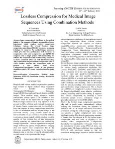
Let us illustrate the behaviour of the proposed FH-3 compression algorithm on the standard grey-level testing image Lena of size 256×256×8 bits, see Fig. 9. Selected bit-planes of the original and compressed image are shown in Fig. 10. Note that the compression is more effective on bit-planes corresponding to more significant bits as there are usually less changes there. Look how well the residuals express perceptually significant features in the image. The mentioned experiment is quantified in Table 2. Notice how the number of residuals increases from the most significant bit-plane to the least significant bit-plane. It is difficult to represent randomness by the estimator. The estimativness ec gives a clear insight into the

V. Hlav´acˇ and J. Fojt´ık

350

Figure 9. Lena — grey level test image

behaviour of the predictor. Cell 6 and 4 from the neighbouring bit planes contain the highest amount of information. Table 2. Quantitative description of the FH-2 and FH-3 methods Bit-plane

bit 7

bit 6 bit 5

bit 4

bit 3

bit 2

bit 1

bit 0

FH-2 residuals 2010 5477 10177 15067 21865 28595 31771 32214 FH-3 residuals empty 3841 5935 9421 15045 21690 28622 31272 estimativness e1 estimativness e2 estimativness e3 estimativness e4 estimativness e5 estimativness e6 estimativness e7

empty empty empty empty 0 1457 0

25 616 52 1892 14 2097 23

160 2165 180 4101 123 3477 118

218 3108 219 5543 143 4169 136

233 4930 233 6611 92 5807 170

91 4919 91 6600 26 5031 85

125 2521 128 2813 112 2312 71

320 457 352 447 361 467 220

The proposed adaptive compression method FH-Adapt was compared on several images from the standard JPEG image set [2]. The methods used for comparison were: Segment from [8], Portable Video Research Group at Stanford PVRG-JPEG from [5], Rounding transform from [6], and Logic coding from [5]. Results were taken directly from the papers. The only implementation that was available was that of Callic [11]. The quantitative measure used for comparison of the different methods is the compression efficiency CE [5]

Adaptive Predictor for Lossless Image Compression

351

Original, bit 7

Residual, bit 7

Original, bit 6

Residual, bit 6

Original, bit 5

Residual, bit 5

Original, bit 4

Residual, bit 4

Original, bit 3

Residual, bit 3

Original, bit 2

Residual, bit 2

Original, bit 1

Residual, bit 1

Original, bit 0

Residual, bit 0

Figure 10. Comparison between bit-planes of the original image and bit-planes storing residuals

CE =

total number of input bytes − total number of output bytes · 100% total number of input bytes

The value CE in Table 3 shows how our method performs in comparison with others. The FH-3 method was outperformed only by Segment and PNG in the case of an image of a monkey (Baboon). The reason is that the predictor cannot cope

V. Hlav´acˇ and J. Fojt´ık

352

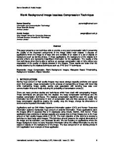
Figure 11. Image of the scanned technical drawing

with the complicated structure of the monkey’s hair. Segment performs also better on the Lena image. Unfortunately we were not able to experiment with Segment because the code was not available. The PNG compression is very similar to the IBM Q80 coder [1]. IBM Q80 is obsolete and the implementation was not accessible. Table 3. Compression coefficients compared with results of others Method/Image PVRG-JPEG Logic Segment Rounding Tr. PNG FH-3

Lena

Baboon

22.7-29.4 6.7-13.7 26.1 12.6 54.6 36.3 37.6 empty 20.7 41.7 34.0 19.1

Boats 24.9-33.1 29.3 empty empty 33.7 41.2

The Table shows the comparison of our method FH- Adapt with other common methods on the Lena image and on a technical drawing image, see Fig. 11. The latter image is perfectly suited for our compression method as can be seen from the results. Table 4. Compression with typical compression methods Type of data Uncompressed ZIP ARJ PCX GIF FH-Adapt.

Lena [Bytes] CE Lena [%] Drawing [bytes] CE Drawing [%] 262656 225007 228389 274256 278771 175434

0 15.62 14.35 -2.85 -4.54 34.21

106940 10224 10380 38624 17290 7297

0 90.44 90.29 63.88 83.83 93.18

Table 5 illustrates the influence of three residual coding methods on three different predictors. This gives us an understanding what improvement the individual

Adaptive Predictor for Lossless Image Compression

353

method brings. The values in the table are the lengths of the compressed 512 × 512 image Lena in bytes. Table 5. Comparison of three proposed predictors and three types of coding techniques. Values are given in bytes Method/Coding Exp. code only Fixed Huffman FH-2 FH-3 FH-Adapt

203000 178655 178130

200758 176021 175541

Moving Huffman 200599 175922 175432

Tests were performed on an Intel Pentium 120MHz computer. The computation time was obtained using a RAM disk to avoid randomness in accessing the disk. The compression of the image Lena (512 × 512 × 8 Bits) takes 6.2 seconds using FH-3 method. The decompression is approximately twice as fast, i.e. in the Lena case it runs 2.7 seconds. Loading/Storing a data without compression takes 0.1 seconds. 9. Conclusions We have proposed a new lossless image compression method that in many respects outperforms other methods considered as state of the art. The basic idea of the method is to predict differences in one bit only. The advantages are: 1. The performance in terms of compression efficiency is similar or better compared to the best methods used. Especially good results were obtained for binary images, grey-level cartoons and man-made drawings. 2. The quick implementation is possible since the operations used are very simple, e.g. SHL, XOR, ADD, and the selection from a table. 3. Substantial parts of the compression and decompression phases can run in parallel. 4. The predictor that constitutes the core of the method can be extended to handle more degrees of the freedom, e.g. to colour images or image sequences. 5. When the resolution of the image increases, the compression ratio does not degrade. This happens in the case of pyramidal algorithms, e.g. MLP (Multi Level Progressive) [3]. The disadvantages of the method are:

354

V. Hlav´acˇ and J. Fojt´ık

1. The compression algorithm needs at least two passes through the image data. When the Huffman coding is used to encode the residuals from the predictor an additional pass is needed. 2. The decompression algorithm is very sensitive to errors in the compressed data. Of course, this disadvantage holds for most compression methods. We encourage the reader to test the method, see the www page http://cmp.felk.cvut.cz/˜fojtik/. Acknowledgements We are grateful to M. I. Schlesinger from Institute of Cybernetics, Ukrainian Academy of Sciences Kiev, Ukraine. His series of lectures held in Prague in summer semester 1996 initiated research reported in this article. J. Matas suggested us a few improvements and K. Johnson carefully read the manuscript. This research was supported by the Czech Ministry of Education grant VS96049, the Grant Agency of the Czech Republic, grants 102/97/0480, 102/97/0855 and the European Union grant Copernicus CP941068.

References [1] ISO/IEC 10918-1: Information technology-digital compression and coding of continuous-tone still images: requirements and guidelines, 1994. [2] Arps, R. B., Truong, T. K.: Comparision of international standards for lossless still image compression. Proc. IEEE 82, 889–899 (1994). [3] Frydrych, M.: Image compression methods. Master’s thesis, Faculty of Mathematics Physics, Charles University, Prague, 1993. [4] Hlav´acˇ , V., Fojt´ık, J.: Adaptive non-linear predictor for lossless image compression. In: Proceedings of the Conference Computer Analysis of Images and Patterns’97, Kiel, Germany (Sommer, G., Daniilidis, K., Pauli, J., eds.), pp. 279–288. Berlin Heidelberg New York Tokyo: Springer, 1997. [5] Chaudhary, A. K., Augustine, J., Jacob, J.: Lossless compression of images using logic minimization. In: Proceedings of the International Conference on Image Processing, vol. II (Delogne, P., ed.), pp. 77–80. Louvain-La-Neuve: IEEE Signal Processing Society, 1996. [6] Jung, H. Y., Choi, T. Y., Prost, R.: Rounding transform for lossless image coding. In: Proceedings of the International Conference on Image Processing, vol. II (Delogne, P., ed.), pp. 65–68. [7] Melichar, B.: Textov´e informaˇcn´ı syst´emy (in Czech) (Text information systems). Faculty of Electrical Engineering, Czech Technical University: Prague, 1996. [8] Ratakonda, K., Ahuja, N.: Segmentation based reversible image compression. In: Proceedings of the International Conference on Image Processing, vol. II (Delogne, P., ed.), pp. 81–84. LouvainLa-Neuve: IEEE Signal Processing Society, 1996. [9] Schlesinger, M. I.: Matematiceskie sredstva obrabotki izobrazenij (Mathematic tools for image processing). Kiev: Naukova Dumka, 1989. [In Russian] [10] Thomas, B. et al.: PNG (portable network graphics) specification version 1.0. Available on http://www.w3.org/Graphics/PNG/, 1996. [11] Wu, X.: Lossless compression of continuous-tone images via context selection, quantization and modelling. IEEE Trans. Image Proc. 6, 656–664 (1997). V. Hlav´acˇ and J. Fojt´ık Center for Machine Perception Faculty of Electrical Engineering Czech Technical University 121 35 Prague 2, Karlovo n´amˇest´ı 13, Czech Republic {hlavac,fojtik}@vision.felk.cvut.cz