Adaptive Probabilistic Flooding for Information Hovering in VANETs

Adaptive Probabilistic Flooding for Information Hovering in VANETs Andreas Xeros, Marios Lestas, Maria Andreou, Andreas Pitsillides

Abstract—Information Hovering applies in many applications in Vehicular Ad Hoc Networks, where useful information needs to be made available to all vehicles within a confined geographical area for a specific time interval. A straightforward approach is to have all vehicles within the hovering area exchange messages with each other. However, this method does not guarantee that all vehicles within the hovering area will receive the message due to potential partitioning of the network in areas with low traffic density and/or low market penetration rate. To alleviate this problem in this work we propose a scheme which is based on the application of epidemic routing within the hovering area and probabilistic flooding outside the hovering area. Informed vehicles outside the area can serve as information bridges towards partitioned uninformed areas thus leading to high reachability. A unique feature of the proposed protocol is that it is adaptive in the sense that the rebroadcast probability outside the hovering area is adaptively regulated based on estimates of the vehicle density within the hovering area. We evaluate the performance of the proposed scheme using VISSIM. The reference model used in all simulation experiments represents a section of the road network in the cities of Bellevue and Redmond in Washington. The obtained simulation results indicate that the proposed protocol is successful in satisfying its design objectives and that it outperforms other candidate hovering protocols.

I. I NTRODUCTION Many applications in VANETs involve the exchange of information messages which are logically attached to a specific geographic area. For example, in case of an unexpected event such as a traffic accident, or road works it is important for all vehicles residing in the surrounding area to be notified of the hazard in order to take appropriate safety measures. In addition, the information must continue to lie in the area for a specific amount of time so that new vehicles entering the area are notified of the imminent danger. Another example involves commercial enterprizes which wish to advertise their products to possible customers within the transportation network. These enterprizes can take advantage of the existing vehicular adhoc network to disseminate their advertisements in an area around their physical location. In all the aforementioned situations, useful information must be broadcast to all vehicles in a specific geographical area and this information must remain in the area for a finite time interval dictated by the application, in order to notify new drivers entering the area of this useful information. The requirements as described above are closely related to the more general concept of information hovering. This work was partly funded by the RPF EM-VANETs project. Marios Lestas and Andreas Pitsillides are with the Computer Science Department of the University of Cyprus, P.O. Box 20537 1678, Nicosia Cyprus. lestas, Andreas.Pitsillides @cs.ucy.ac.cy Andreas Xeros and Maria Andreou are with the School of Science and Engineering of the Open University of Cyprus,

[email protected], [email protected]

The term Information Hovering was first introduced in [8], and formally defined later in [7]. A more detailed description is provided in [1]. The concept involves decoupling of the hovering information from its host and promotes coupling it directly with a specific geographical location which is called the anchor location. In this regard, the hovering information stays ”attached” to a specific geographical area (called the anchor area). The information hovers from one mobile device to another, in a quest to remain within a specific vicinity and avail itself to users currently present or entering its anchoring geographical location. The Information Hovering concept can be used in a variety of applications in Mobile Adhoc Networks with characteristic usage examples provided in [3]. A relevant concept in the networks literature is Geocasting, which addresses the problem of information dissemination in geographical target regions. Geocast protocols which have appeared in the literature [5] are intended to forward the relevant message in the target region and distribute the message once, to all devices residing in the region. However, this one time message delivery is not relevant in the ’information hovering’ paradigm, as the information needs to remain in the target area for a specific amount of time. This concept has appeared in the literature as abiding or time-stable geocasting [4]. Flooding based schemes, such as epidemic routing [6] can be applied to the entire network to effectively serve such a paradigm, achieving high percentage of nodes in the hovering area receiving the relevant message (high reachability). However, this is done at the expense of a large number of redundant messages which strain the communication channel and lead to extensive contention and large latency of message delivery. In order to make efficient use of the available resources and substantially reduce the number of exchanged messages, one may choose to apply epidemic routing merely in the hovering area. However, this approach may also reduce the achieved reachability in cases of low traffic density. Low traffic density in the hovering area may cause the network to become intermittently connected. This implies that sections of the network within the hovering area which are partitioned from the information sources may never receive the messages, thus decreasing the achieved reachability. This demonstrates that the design of information hovering protocols is highly challenged by the intermittently connected nature of the network in cases of low traffic densities. One approach to address this challenge is to allow controlled exchange of messages outside the hovering area. The reasoning behind this approach is that informed vehicles outside the hovering area can serve as information bridges towards partitioned uninformed areas, thus increasing message reachability. In addition, since ’epidemic routing’ outside the hovering area is avoided, the number of exchanged messages is reduced. The authors in [2] follow this

reasoning to allow epidemic dissemination of messages in an extended area beyond the hovering area. They demonstrate through simulations that such an approach can increase the recorded reachability in cases of low traffic density. In this work we adopt an alternative approach which involves employing epidemic routing inside the area and probabilistic flooding outside the hovering area. Our approach allows controlled exchange of messages in the entire network thus offering a wider choice of available paths towards the hovering area leading to increased reachability. We demonstrate through simulations that our approach outperforms the scheme proposed in [2] by significantly decreasing the number of messages required in order to achieve high reachability. The design methodology has been simulative and a major challenge in the overall procedure has been the design of the rebroadcast probability function. Among a number of candidate functions, we choose the one which yields superior performance and we tune its parameters taking advantage of phase transition phenomena which are typical in probabilistic flooding schemes. A unique feature of the proposed protocol is that it is adaptive in the sense that the rebroadcast probability outside the hovering area is adaptively regulated based on estimates of the vehicle density within the area. Estimates of the vehicle density within the hovering area are obtained using measurements of the number of neighbors of each vehicle. The formula relating the two quantities is derived using a simple model of the transportation network within the hovering area. We demonstrate through simulations that the proposed scheme is successful in satisfying the design objectives and outperforms other candidate hovering protocols such as epidemic routing in the entire network, epidemic routing in the hovering area only and the scheme proposed in [2]. The rest of this paper is organized as follows. In section II we present the adopted methodology leading to the development of the proposed information hovering protocol, in section III we derive and validate the formula which relates the vehicle density within the hovering area and the number of neighbors of each vehicle, in section IV we evaluate the performance of the proposed scheme using simulations and finally in section V we offer our conclusions and future research directions. II. P ROPOSED T RAFFIC A DAPTIVE I NFORMATION H OVERING P ROTOCOL A straightforward solution to the information hovering problem is the application of epidemic routing merely within the hovering area. However, this approach, as discussed in the introduction, leads to low reachability in cases of low traffic density. Low traffic densities cause the network to become intermittently connected and partitioned uninformed areas are impossible to receive the critical information data. In such a scenario, vehicles outside the hovering area can serve as information bridges towards the partitioned uninformed areas. One can thus increase the achieved reachability by allowing epidemic routing in the entire network. This however, leads to a huge number of redundant messages. For this reason, in this work we present a solution which employs epidemic routing

within the hovering area and probabilistic flooding outside the hovering area. Since epidemic routing outside the hovering area is avoided, the number of exchanged messages is greatly reduced. The proposed information hovering protocol works as follows: We assume that all vehicles are equipped with a positioning system such as GPS. Vehicles exchange beacon messages which enable them to discover their neighbors. The information sources within the hovering area, initiate the dissemination process by broadcasting a packet which includes the critical message and the following fields in its header: a TTL field which determines the expiration time of the message and a hovering area field which contains information which can be used to determine the hovering area. They then mark all vehicles currently in their neighbor list as recipients of the critical message. A vehicle upon receiving the packet, stores the critical message and the fields contained in the packet header and checks whether it resides within the advertised hovering area. If it does lie in the hovering area, it periodically checks whether its neighbors have been marked as recipients of the critical message. The frequency with which the check is conducted, is referred to as the scanning frequency. If there exists at least one neighbor which has not received the critical message, then the vehicle decides to rebroadcast the message and marks all neighbors as recipients of the critical message. If the vehicle does not lie within the hovering area, it decides to initiate the rebroadcast procedure with probability p and decides to reject the received message with probability 1 − p. The probability p is calculated based on a probability function f . This function can have several input variables however, in this work we restrict our choices to decreasing functions of the distance from the hovering area only. The reason behind this design choice is that the further an informed vehicle is from the hovering area, the less probable it is, that it will contribute to the finding of a yet unexplored path. The TTL field in the packet header is used to determine the expiration time of the critical message. When a packet is received, the value in the TTL field is stored locally and periodically decreased. If the vehicle decides to rebroadcast the critical message it stores the updated local value in the corresponding TTL field. The most significant part of the overall design procedure is the determination of the probability function f . In this work, the method used to determine this function has been simulative. Our initial objective has been to determine the type of function to be utilized, and our subsequent efforts focus on tuning its parameters. The probability function, as discussed above, is required to be non-increasing. We thus consider four commonly used non-increasing candidate functions which we evaluate using simulations in order to select the one which exhibits superior performance. The candidate functions chosen are the following: • Gaussian-like function: d2

p = e− 2σ2 •

(1)

Linear function: p=1−

1.3d 3r

(2)

•

Exponential-Like function: p = e−

0.7d r

(3) A

Step function:                   p=

                

1 0.90 0.80 0.70 0.60 0.50 0.40 0.30 0.20 0.10 0

if if if if if if if if if if if

D

d ≤ ( 9r ) ( 9r ) < d ≤ ( 4r ) ( 4r ) < d ≤ ( 2r ) ( 2r ) < d ≤ ( 7r 9 ) 17r ( 7r ) < d ≤ ( 9 18 ) 17r ( 18 ) < d ≤ ( 10r 9 ) 13r ( 10r ) < d ≤ ( 9 9 ) 5r ( 13r ) < d ≤ ( 9 3 ) ( 5r ) < d ≤ (2r) 3 (2r) < d ≤ ( 43r 18 ) d > ( 43r ) 18

E

Transmission Probability

1.2 1

Gaussian Exponential

0.6

Linear Step

0.4 0.2

682

651

620

589

558

527

496

465

434

403

372

341

310

279

248

217

186

155

93

124

62

0

0 31

F

B

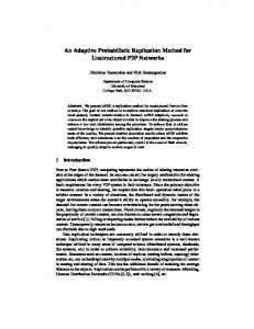
Fig. 2. Road map of the reference model used in all simulation experiments. It represents a section of the road network in the cities of Bellevue and Redmond in Washington. Hovering areas are marked as black circles.

where σ, d and r are design parameters. These parameters are tuned so that the candidate probability functions exhibit similar decreasing behavior as shown in Fig. 1.

0.8

C

(4)

Distance of Receiver from Hovering Area (m)

Fig. 1. Candidate probability functions. Their parameters have been tuned to exhibit similar decreasing behavior.

The reference model used in all simulation experiments, represents a section of the road network in the cities of Bellevue and Redmond in Washington. It includes congested arterial streets and a saturated freeway as shown in Fig. 2. The modeled freeway includes lanes for general traffic, HOV/Bus lanes, 3 closely spaced interchanges, 6 ramp meters, and 2 collector-distributor roads. We identify 6 hovering areas in this road network which are shown in Fig. 2 and for this set of experiments we consider area A. We conduct all the simulation experiments using VISSIM [9], a microscopic simulation tool. The four candidate probability functions are integrated in the information hovering protocol described above, and the resulting schemes are evaluated in terms of the average reachability achieved and the total number of messages received by the vehicles. The average reachability is calculated over the simulation time after which the system has settled down to its equilibrium state. The performance of the four schemes is also compared with two other protocols which can be considered as extreme cases of the class of probabilistic hovering protocols which can be designed: epidemic routing in the entire network which implies a probability function equal to 1 and epidemic routing in the hovering area only, which implies a probability function equal to 0. Epidemic routing in the entire network yields high reachability at the expense of a large number of

redundant messages whereas epidemic routing in the hovering area only achieves a low number of exchanged messages at the expense, however, of reduced reachability in cases of low traffic densities. The performance of the considered information hovering schemes is investigated in area A for different values of the traffic density. We consider traffic density values in the range 2.3 - 9.2 Vehicles/Km2 . Fig. 3 shows the number of received messages, whereas Fig. 4 shows the corresponding reachability values. As expected, the highest reachability is reported by the epidemic routing scheme at the expense however, of the highest number of exchanged messages. On the other end, epidemic routing within the hovering area and the linearly decreasing probability function report the lowest reachability values. The remaining protocols exhibit similar reachability values close to the one achieved by epidemic routing. The Gaussian-like probability function however, reports the smallest number of exchanged messages and is thus the probability function of choice for the information hovering protocol to be designed.

350 Number of Messages

•

300 Epidemic in Area

250

Linear

200

Step

150

Exponential Normal

100

Epidemic

50 0 0

1

2

3

4 T

a r

fci

D

e

5 n

6

7

8

9

10

tsiy

Fig. 3. Number of messages exchanged in area A for each of the candidate probability functions.

Having decided on the type of function to be used, the next step is to tune the parameters of this function in order to achieve the best possible performance. The equation of the chosen Gaussian-like probability function is given by equation 1. This equation is obtained by considering a normal curve d2 p = σ√12π e− 2σ2 with mean equal to zero and standard deviation equal to σ, which is then multiplied by a factor

60 120

50 Epidemic in Area

80

Linear 60

Step

40

Exponential Normal

20

Epidemic

0 0

1

2

3

4

5

6

7

8

9

10

Number of Messages

Reachability

100

40 30 20

10 0 0

45

90

135

180

Fig. 4. Reachability achieved in area A for each of the candidate probability functions.

σ 2π. The latter multiplication is necessary to ensure that the transmission probability on the boundary of the hovering area is equal to 1. The standard deviation σ is the only parameter of the function whose value needs to be regulated. The value of σ is a measure of the area in which critical message forwarding is allowed with high probability. The size of this area and thus the value of σ must be adaptively regulated based on the connectivity of the network within the hovering area. The smaller the connectivity is, the larger σ must be, in order to provide more message forwarding opportunities. More message forwarding opportunities enable additional paths to be explored which in turn lead to increased connectivity and thus high reachability. However, the connectivity within the hovering area is a difficult quantity to measure directly and so the value of σ is adaptively regulated based on network parameters which affect the achieved connectivity and their values are either known or estimated online. One such parameter is the transmission range of each vehicle. In this work we assume that the transmission range is constant to a value of 180m which is typical in vehicular ad hoc networks. The effect of the transmission range on the derived results will be the topic of future research. Another parameter which is known to affect network connectivity is the vehicle density within the hovering area. The higher the vehicle density is, the higher is the probability of high connectivity and so a lower value of σ suffices to guarantee high reachability and low number of exchanged messages. The exact function, mapping the vehicle density to the desired value of σ is determined using simulations. Various vehicle density values are considered in area A and for each vehicle density, the value of σ which yields the best possible performance is extracted. Despite the fact that the original simulation study is conducted in area A, the same design procedure is later applied in other hovering areas demonstrating the robustness of the derived function with respect to changing topologies. In order to characterize the value of σ which yields, for a particular traffic density, the best possible performance, the traffic density in area A is first set equal to 2.9 V eh/Km2 and the number of received messages and the reachability achieved by the proposed information hovering protocol are recorded for a predetermined set of values of σ in the range 0 to 540. The recorded values are shown in Fig. 5 and Fig. 6 respectively. We observe an almost linear increase in the number of

270

315

360

405

450

495

540

Sigma (m)

Fig. 5. Number of messages exchanged in hovering area A for different values of σ when the vehicle density is set to 2.9Veh/Km2 .

100 90 80 70 Reachability

√

225

60 50 40 30 20 10 0 0

45

90

135 180

225

270 315

360 405

450

495 540

Sigma (m)

Fig. 6. Reachability achieved in hovering area A for different values of σ when the vehicle density is set to 2.9 Veh/Km2 .

messages as the value of σ increases. In addition, the achieved reachability also increases with increasing σ until, a critical value is reached, beyond which the reachability is almost constant attaining values close to 100%. For a particular vehicle density, this critical value of σ is the desired one, as it achieves high reachability, with the minimum possible number of exchanged messages. The existence of this critical value is a strong indication of the presence of phase transition phenomena which are typical in the theory of percolation theory and random graphs. The same type of behavior is observed in other hovering areas and for different traffic density values. Fig. 7 shows the achieved reachability vs the number of exchanged messages when the vehicle density in area B is set to 21 Veh/Km2 whereas Fig. 8 shows the achieved reachability vs the number of exchanged messages when the vehicle density in area C is set to 4.3 Veh/Km2 . Each point on these graphs corresponds to a particular value of σ. However, due to the strictly increasing relationship between σ and the number of exchanged messages, higher values of exchanged messages also imply higher values of σ. We consider values of σ in the range 0-540. A value of σ equal to zero corresponds to the application of epidemic routing in the hovering area only. We also consider the application of epidemic routing in the entire network which corresponds to a value of sigma equal to ∞. The graphs indicate the existence of a critical value of σ, beyond which the achieved reachability is almost constant.

σ=90

σ=45

σ=0

σ=inf

σ=225

90 80

Reachability

500 400

Area A Area B

300

Area C Area D

200

Area E Area F

100

Least Squares Fit

0 0

5

10

15

20

25

30

35

-100 Traffic Density (Veh in Km2)

Fig. 9. Critical value of sigma vs traffic density graphs in different hovering areas. We observe similar behavior in all hovering areas. The relationship used in the proposed protocol is obtained by applying a least squares fit between the curves.

rebroadcast probability outside the hovering area. The metric used in this work to estimate the vehicular density, is the average number of neighbors of the vehicles residing in the hovering area. But how does the vehicular density relate to the average number of neighbors in a roadway setting? The plethora of possible roadway topologies make any general analysis intractable, so in this work we derive the relationship theoretically considering the simple case of two, two-way straight roads crossing perpendicularly at the center of the circular hovering area as shown in Fig. 10.

110 100

600

Critical Sigma

Such critical density values are obtained for values of the traffic density in the range 2 -25 Veh/Km2 in all hovering areas depicted in Fig. 2. The extracted critical σ values vs the traffic density are shown graphically in Fig. 9. We observe that the relationship between the desired σ and the vehicle density exhibits an exponentially decreasing behavior which is similar in all hovering areas. This demonstrates that the relationship is almost independent of the considered topology which implies that a universal σ vs vehicle density function can be derived. We derive such a function by considering a least squares fit between the curves. The resulting function is shown graphically in Fig. 9. The vehicle density within the hovering area is an unknown quantity which needs to be estimated online. In the subsequent section we discuss the estimation method.

70 60 50 40 30 0

50

100

150

200

250

300

350

400

I2

Number of Messages

Area A

Fig. 7. Reachability vs number of message exchanged in hovering area B, for different values of σ when the traffic density is set to 21V eh/Km2 .

Area B

r

r

I4

I1

I3

Area C R

75 σ=540

70

σ=450

σ=inf

65 Reachability

60 σ=360

55

I5

σ=225

50

Fig. 10. The road topology of the model used to relate analytically the vehicle density with the average number of neighbors.

σ=90

45 40

σ=0

35 30 0

5

10

15

20

25

30

35

40

45

50

Number of Messages

Fig. 8. Reachability vs number of message exchanged in hovering area C, for different values of σ when the traffic density is set to 4.3V eh/Km2 .

III. E STIMATION OF THE V EHICLE D ENSITY The vehicle density within a confined area is a global quantity which is impossible to calculate accurately in a distributed fashion, in cases where the vehicular network is intermittently connected. Since in the considered scenarios the vehicular network is often partitioned, distributed algorithms must be developed to estimate the quantity online. As described in the previous section, these estimates are required by the developed information hovering protocol to calculate the

Our objective is to calculate the expected number of neighbors of each vehicle when the number of vehicles residing in the hovering area is equal to n+1. In such a case the vehicle density is given by n+1 πR2 where R is the radius of the hovering area. We assume that at any time instant the location of each vehicle is a uniformly distributed random variable over all possible locations in the considered roadway system. Two vehicles are considered to be neighbors when they lie within their transmission range. It follows from our previous assumption that the events of any two vehicles being neighbors are independent. The event of any two vehicles being neighbors is a bernoulli trial with probability of success equal to p. It follows from the independence of the bernoulli trials that the number of neighbors of any vehicle is a binomially distributed random variable whose expected value is equal to np. So, in order to calculate the expected number of neighbors when the number of vehicles in the hovering area is equal to n + 1, it

suffices to calculate the probability p of two vehicles being neighbors. We calculate this probability below. We first define basic notations utilized in the subsequent analysis. As mentioned above we assume that in the considered hovering area, the roadways systems consists of two two-way straight-line roads intersecting perpendicularly. I1 represents the point of intersection where I2 up to I5 represent the edge-points on the considered roadway system as shown in Fig. 10. Among the n + 1 vehicles residing in the hovering area, we randomly select two, referred to as veh1 and veh2 and our objective is to calculate the probability that the distance between these vehicles is less than their transmission range r which is assumed to be constant. hi−j represents the directional roadway link between points Ii and Ij . The direction of the traffic flow is from Ii to Ij . We partition the hovering area in three subareas A, B, C as shown in Fig. 10. Area A represents the circular ring enclosed by the perimeters of the concentric circles with radius R and R − r respectively, Area B represents the circular ring enclosed by the perimeters of the concentric circles with radius R − r and r respectively, and area C represents the circle with radius r. The probability of vehicle veh1 residing in area A is denoted by P1A . In a similar way we define P1B and P1C . Given that veh1 lies in area A, the probability that it has veh2 as a neighbor is constant and is denoted by P nA . Similarly we define P nB and P nC . Due to the areas A, B and C constituting a partition of the hovering area, the desired probability p is given by p = P1A ∗ P nA + P1B ∗ P nB + P1C ∗ P nC

(5)

Probability P1A is equal to the ratio of the total road segment lying in area A over the total road segment within the hovering area. Since the road is bidirectional, the length of the road segment in Area A is given by 8r, whereas the total length of the road segment within the hovering area is given by 8R. It follows that: r R Similarly, one can deduce that: P1A =

j=2

A A to the symmetry of the problem P nA 1−j = P nj−1 = P n1−2 1 A A ∀ j = {2, 3, 4, 5} and P1−j = Pj−1 = 8 ∀ j = {2, 3, 4, 5}. It follows that:

1 3r ∗ P nA (9) 1−2 ∗ 8 = 8 8R In area B, given that the veh1 is placed on road h1−2 , then veh2 will be a neighbor of veh1 if it is less than r apart from veh1 in both directions on h1−2 or in road h2−1 . In 4r this case P nB (k) is equal to 8R and P nB 1−2 is given by ∫ R−r 1−2 1 4r B P n (k)dk = . Using the same arguments 1−2 R−2r r 8R leading to equation (9), it follows that P nA =

1 r ∗ P nB (10) 1−2 ∗ 8 = 8 2R Finally, when veh1 is placed in area C on road h1−2 , then veh2 will be its neighbor if it lies a distance less than r from veh1 on roads h1−2 and h2−1 . In addition, assuming that veh1 is located a distance k from intersection I1 on road h1−2 , then veh2 can √ be a neighbor of veh1 if it is located within a distance r2 − k 2 from I1 on roads h1−3 , h3−1 , h1−4 , h4−1 . So, given that veh1 is in area C, the probabilC ity that the two vehicles are neighbors √ P n1−2 is given by √ ∫ ∫ 2 2 r r −k r 4r r 1 k 2 . By setting 8R + 4 0 8Rr dk = 2R + 2Rr 0 r 1 − ( r ) √ π ∫ r k 1 C 2 n1−2 = 2R + 2Rr r 0 1 − sin2 θ r = sin θ, we get: P π ∫ r r r rπ 2 1 + cos 2θdθ = 2R r cos θdθ = 2R + 4R + 8R = 4r+rπ 8R . 0 Using the same arguments leading to equation (9), it follows that P nB =

(6)

R − 2r (7) R r P1C = (8) R We now calculate the probability of P nA . Given that veh1 is in area A, we assume, that it is located on road h1−2 distance k from the perimeter of the area and in this case denote by P nA 1−2 (k) the probability that veh2 is its neighbor. k can attain values between 0 and r and so the conditional probability that veh1 has veh2 as its neighbor when lies on road h1−2 within ∫ it A 1 r P n area A, P nA , is given by 1−2 (k)dk. veh2 will be 1−2 r 0 neighbor of veh1 in two cases: if it is located on any side of the road between veh1 and I2 and if it is located on any side of the road within a distance r from veh1 in between veh1 and I1 . The probability that the first case is valid is equal to the length of the roadway section between veh1 and I2 over the total length of the roadway in the hovering area, whereas the P1B =

probability of the second case being valid due to its geometry 2r 2k is equal to 41 P1A . So, ∫P nA 1−2 (k) is equal to 8R + 8R and 1 r 3r A A P n1−2 is given by r 0 P n1−2 (k)dk = 8R . Similarly we A define P nA 1−j and P nj−1 for j = {2, 3, 4, 5}. Moreover, we A A define P1−j and Pj−1 j = {2, 3, 4, 5} to be the probabilities that veh1 lies in road section h1−j , hj−1 respectively in area 5 ∑ A A A A. It follows that P nA = P nA 1−j P1−j + P nj−1 Pj−1 . Due

1 4r + rπ ∗ P nC 1−2 ∗ 8 = 8 8R Substituting equations (6)-(11) in (5) we obtain P nC =

(11)

r 3r R − 2r r r 4r + rπ 4Rr + πr2 − r2 + + = R 8R R 2R R 8R 8R2 (12) which implies that the expected number of neighbors E[X], where X denotes the random variable of the number of neighbors of a vehicle in the hovering area, when the vehicle density is equal to n+1 πR2 is given by: p=

4Rr + πr2 − r2 (13) 8R2 The above probability is derived using a simple model of the roadway system which consists of two intersecting roads only. In the remainder of this section we compare our theoretical findings with simulation results which are extracted from scenarios which relax the simplifying assumptions of our theoretical model. We observe striking agreement between E[X] = n

the theoretical findings and the simulation results despite the simplicity of the theoretical model. The reference model used in the simulation experiments is the one considered in the previous section, which is shown in Fig. 2. We utilize all the hovering areas (A-F). All hovering areas have identical topology, being circular with radius R = 500m. The roadway topologies within the hovering areas, however, differ significantly and are more complex than the one of the theoretical model, involving a considerable number of intersecting roads. In all simulation experiments, the vehicle transmission range r is set equal to 180m. In each hovering area, we consider various values for the number of vehicles residing in the area and for each number we use the simulation results to find the average number of neighbors. We compare these results with the function of equation 13 which becomes E[X] = 0.21n when R and r are assigned their values. The results are shown in Fig. 11. We observe very good agreement between the simulation results and our theoretical findings. This demonstrates the validity of equation 13 and that it can be successfully used in the proposed hovering scheme to accurately estimate the vehicle density within the hovering area, when the average number of neighbors is known priori. The average number of neighbors in the hovering area can be calculated via exchange of beacon messages between vehicles. Each vehicle maintains a list of its neighbors which it discovers via the exchange of hello messages. It also maintains a list of the neighbors of each of its neighbors. The average number of neighbors in the hovering area is then calculated by each vehicle using a weighted moving average algorithm which takes into account all the aforementioned local variables. Details of the beacon exchange mechanism and the weighted moving average calculation are omitted due to lack of space but will be included in an extended version of the paper to be soon made available online.

Average Number of Neighbors

4 3.5 Area A

3

Area B 2.5

Area C

2

Area D Area E

1.5

Area F

1

Theory

0.5 0 0

5

10

15

20

Average Number of Vehicles in the Hovering Area

Fig. 11. Average number of neighbors obtained using simulations in different hovering areas, for different average number of vehicles in the areas and comparison with the predicted values using equation (13)

IV. P ERFORMANCE EVALUATION In this section we evaluate the performance of the proposed information hovering protocol using simulations. The reference model used is drawn from the same area considered in the design procedure i.e. a section of the road network in the cities of Bellevue and Redmond in Washington. However,

G

H

Fig. 12. Road topology of the reference model used to evaluate the performance of the proposed information hovering protocol. The considered hovering areas are marked on the diagram as circles.

we consider different hovering areas than the ones used in the design procedure which are shown in Fig. 12 denoted by the letters H and G. The performance metrics used are the reachability within the hovering area and the number of received messages. As discussed in previous sections the design objective has been to achieve the highest possible reachability with the minimum number of exchanged messages. We first conduct a comparative study in order to investigate to what extent the proposed scheme achieves its design objectives relative to other schemes which have appeared in the literature: epidemic routing in the hovering area only, epidemic routing in the entire vehicular network and the scheme proposed in [2] which allows exchange of messages in a closed area outside the hovering area. Since the authors in [2] do not give guidelines on how to choose the size of this area, we have set the extended area to be equal in size to the hovering area. This is achieved by setting the radius √ of the area in which message exchange is allowed, equal to 2 times the radius of the hovering area. The number of exchanged messages and the reachability reported in area H are shown in Fig. 13 as we increase the average number of vehicles residing in the area. We observe that for low traffic densities, the reachability achieved by the four schemes is significantly less than 100% indicating the existence of partitioned areas which prevent some vehicles to be informed of the critical message. As the vehicle density increases, both the achieved reachability and the number of exchanged messages increases. However, we observe that the proposed adaptive probabilistic flooding scheme, exhibits superior performance as it achieves high reachability values, close to the ones reported by the scheme which applies epidemic routing in the entire network and low number of exchanged messages, similar to the ones reported by the scheme which applies epidemic routing in the hovering area only. The proposed scheme thus gets the best of the two aforementioned schemes. The extended hovering area approach, is successful in achieving high reachability values, at the expense however, of a much larger number of exchanged messages. Similar results are obtained in area G which are shown in Fig. 14. This demonstrates the ability of the proposed scheme to work effectively in various hovering areas with different road topologies and traffic characteristics.

450

450

400

350 300

Adaptive Prob. Flooding

250

Blind Floding

Number of Messages

Number of Messages

400

200 Blind Flooding In the Area

150 100

300

Blind Flooding

250 200 150

Blind Flooding in the Area

100

Extended Area

50

Extended Area

50

Adaptive Prob. Flooding

350

0

0 0

5

10

15

20

0

25

5

110 100 90 80 70 60 50 40 30 20 10 0

Adaptive Prob. Flooding Blind Floding Blind Flooding In the Area Extended Area

5

10

15

20

15

20

(a) Number of Exchanged Messages

Reachability

Reachability

(a) Number of Exchanged Messages

0

10

Average Number of Vehicle in the Area

Average Number of Vehicles in the Area

25

110 100 90 80 70 60 50 40 30 20 10 0

Adaptive Prob. Flooding Blind Flooding Blind Flooding in the Area Extended Area

0

5

10

15

20

Average Number of Vehicle in the Area

Average Number of Vehicles in the Area

(b) Reachability

(b) Reachability

Fig. 13. Comparison of the proposed adaptive probabilistic scheme with other hovering schemes in terms of the reachability achieved and the number of messages exchanged in area H, for different average number of vehicles in the area.

Fig. 14. Comparison of the proposed adaptive probabilistic scheme with other hovering schemes in terms of the reachability achieved and the number of messages exchanged in area G, for different average number of vehicles in the area.

V. C ONCLUSIONS AND F UTURE W ORK In this paper we address the Information Hovering problem in VANETS. Similar to many problems in VANETS, the performance of the information hovering protocol is affected by the traffic density of the considered transportation network. In cases of low traffic density, partitioned uninformed areas may lead to low traffic density. In this work, we propose a novel scheme which overcomes this problem by applying probabilistic flooding outside the hovering area. Informed vehicles outside the area can serve as information bridges towards partitioned uninformed areas thus leading to high reachability. A unique feature of the proposed protocol is that it is adaptive in the sense that the rebroadcast probability outside the hovering area is adaptively regulated based on estimates of the vehicle density within the hovering area. Simulation results indicate that the proposed protocol is successful in satisfying its design objectives and that it outperforms other candidate hovering protocols which have appeared in the literature. A major challenge is the establishment of analytical results to support our simulative findings. We aim at addressing this problem using tools from random graph theory. R EFERENCES [1] G. Di Marzo Serugendo, A. Villalba Castro and D. Konstantas. ”Dependable Requirements for Hovering Information”. In Supplementary

[2]

[3] [4]

[5] [6] [7]

[8] [9]

Proceedings of the 37th Annual IEEE/IFIP International Conference on Dependable Systems and Networks, (DSN’07), June, 2007. S. Hermann, C. Michl and A. Wolisz. ”Time-Stable Geocast in Intermittently Connected IEEE 802.11 MANETs”. In the Proc. of IEEE Vehicular Technology Conference (VTC Fall), Baltimore, September 2007. D. Konstantas and A. Villalba. ”Hovering Information : A paradigm for sharing location-bound information”. In European Conference on Smart Sensing and Context, 2006. C. Maihofer, T. Leinmuller and Elmar Schoch. ”Abiding geocast: time-stable geocast for ad hoc networks”. In the Proc. of the 2nd ACM international workshop on Vehicular ad hoc networks (VANET05), pp.20-29 New York, 2005. C. Maihfer. ”A survey on geocast routing protocols”, In IEEE Communications Surveys and Tutorials, 2nd quarter issue, Vol. 6, 2004. A. Vahdat and D. Becker. ”Epidemic routing for partially connected ad hoc networks”. Duke University, Tech. Rep. CS-200006, 2000. A. Villalba, G. Di Marzo Serugendo and D. Konstantas. ”Hovering Information - Self-Organising Information that Finds its own Storage”. In International IEEE Conference on Sensor Networks, Ubiquitous and Trustworthy Computing, Taichung, Taiwan, pp. 193200, June 2008. A. Villalba and D. Konstantas. ”Towards hovering information”. In the Proc. of the First European Conference on Smart Sensing and Context (EuroSSC), pp. 161-166, 2006. The VISSIM traffic simulator. http : //www.ptv.de/cgi − bin/traf f ic/traf vissim.pl, 2007.