Adaptive Real-time Particle Filters for Robot Localization

Adaptive Real-time Particle Filters for Robot Localization Cody Kwok† † Dept.

Dieter Fox†

Marina Meil˘a‡

of Computer Science & Engineering, ‡ Dept. of Statistics University of Washington Seattle, WA 98195

{ctkwok,fox}@cs.washington.edu, [email protected]

Abstract— Particle filters have recently been applied with great success to mobile robot localization. This success is mostly due to their simplicity and their ability to represent arbitrary, multi-modal densities over a robot’s state space. The increased representational power, however, comes at the cost of higher computational complexity. In this paper we introduce adaptive real-time particle filters that greatly increase the performance of particle filters under limited computational resources. Our approach improves the efficiency of state estimation by adapting the size of sample sets on-the-fly. Furthermore, even when large sample sets are needed to represent a robot’s uncertainty, the approach takes every sensor measurement into account, thereby avoiding the risk of losing valuable sensor information during the update of the filter. We demonstrate empirically that this new algorithm drastically improves the performance of particle filters for robot localization.

I. I NTRODUCTION Mobile robot localization is the problem of estimating the location of a robot based on a map and sensor data collected by the robot. Most successful approaches to robot localization are variants of Bayesian filtering, where the robot’s location is represented by posterior densities over the space of all locations [1], [6], [9], [7]. Particle filters represent these posteriors by sets of random samples (see [4] for a recent overview). Due to this representation, particle filters are optimal estimators even for non-linear, non-Gaussian dynamic systems [3]. Furthermore, particle filters can solve the global localization problem, i.e. they can estimate a robot’s position without knowledge of its start location [6], [9], [7]. Unfortunately, the sample-based representation of particle filters comes at increased computational requirements, especially compared to closed-form solutions such as the Kalman filter and its extensions [1], [9], [7]. Computation resources available for an autonomous robot are typically very limited, resulting in common situations where the rate of incoming sensor data is higher than the update rate of the particle filter. The prevalent solution is to update the filter as often as possible and to discard sensor information that arrives during the update process. Obviously, this approach is prone to losing valuable sensor information.

In [8] we introduced real-time particle filters to deal with such situations. Instead of discarding sensor readings, this technique distributes the samples among the different observations arriving during a filter update. Hence posteriors are represented by mixtures of sample sets. By weighting the different sets in the mixture, the approach focuses computational resources (samples) on valuable sensor information. In this paper, we enhance real-time particle filters by adapting the size of the mixture using KLD-sampling [5], a technique that determines the number of samples based on statistical bounds on the samplebased approximation quality. We empirically demonstrate that this approach is superior to alternative algorithms using particle filters for robot localization. The remainder of this paper is organized as follows: In the next section we outline the basics of particle filters and their extensions to real-time domains and adaptive sample sets. Then, in Section III, we present our novel approach to adaptive real-time particle filters. Finally, we present experimental results followed by a discussion. II. PARTICLE FILTERS Particle filters are a sample-based variant of Bayes filters, which recursively estimate posterior densities, or beliefs Bel, over the state xt of a dynamic system [6]: Z Bel(xt ) ∝ p(zt | xt ) p(xt | xt−1 , ut−1 )Bel(xt−1 )dxt−1 Here zt is a sensor measurement and ut−1 is control information describing the dynamics of the system. Particle filters represent beliefs by sets St of N weighted (i) (i) (i) (i) samples hxt , wt i. Each xt is a state, and the wt are non-negative numerical factors called importance weights, which sum up to one. The basic form of the particle filter realizes the recursive Bayes filter according to a sampling procedure, often referred to as sequential importance sampling with resampling (SISR): 1. Resampling: Draw with replacement a random state x from the set St−1 according to the (discrete) distribution (i) defined through the importance weights wt−1 .

(a)

z2

z1

z4

z3

Robot position u 123

S1 Start

S4

(a) (b)

.....

z2

z1

z4

z3

Robot position u123

S1

S4

(b) (c) z2

z1

S1

u1

S2

z3

u2

S3

z4

u3

S4

Robot position Fig. 2. Different strategies for dealing with limited computational

(c) Map of the UW CSE Department along with a series of sample sets representing the robot’s belief during global localization using sonar sensors (samples are projected into 2D). The size of the environment is 54m × 18m. Figures a) – c) show the sample sets after moving 5m, 35m, and 55m, respectively. Fig. 1.

2. Sampling: Use x and the control information ut−1 to sample x0 according to the motion model p(x0 | x, ut−1 ), which describes the dynamics of the robot. 3. Importance sampling: Weight the sample x0 by the observation likelihood w0 = p(zt | x0 ). This likelihood is extracted from a model of the robot’s sensors (e.g. sonar, laser range-finder, camera) and a map of the environment. Each iteration of these three steps generates a sample hx0 , w0 i drawn from the posterior. After N iterations the sample set is complete and the importance weights are normalized so that they sum up to one. In contrast to the extended Kalman filter [1], particle filters can be shown to converge to the true posterior even in non-Gaussian, non-linear dynamic systems [4]. Figure 1 illustrates the application of particle filters to mobile robot localization. Shown there is a map of a hallway environment along with a sequence of sample sets during global localization. The pictures demonstrate the ability of particle filters to represent a wide variety of distributions, ranging from uniform to highly focused. While a large number of samples might be necessary to accurately represent the belief during early stages of localization (cf. 1a), it is obvious that only a small fraction of this number suffices to track the position of the robot once it knows where it is (cf. 1c). Therefore, the efficiency of particle filters can be greatly increased by adapting the number of samples during the localization process, as demonstrated in [5]. When a large number of samples is required, however, another issue arises.

power. All approaches process the same number of samples per estimation interval (window size three). a) Skip observations, i.e. integrate only every third observation. b) Aggregate observations and integrate them in one step. c) Reduce sample set size so that every observation can be integrated.

A. Limited computational power An important assumption underlying particle filters is that all N samples can be updated before new sensor information arrives. However, in early stages of global localization, it is possible that the update cannot be completed before the next measurement arrives. In this paper we present an approach that improves the performance of particle filters by concurrently addressing the following two questions: 1) How can we deal with situations in which the update rate of the filter is lower than the rate of incoming sensor observations? 2) How can we adapt the number of samples on-the-fly so as to optimally use computational resources? Before we focus on the first question, let us introduce some notation. We assume that observations arrive at fixed time intervals. Let N be the number of samples required by the particle filter. An estimation window comprises the time required to update all N samples. We measure the duration, or size, of estimation windows by the number of observations arriving during the window. Hence, a window size of k means that k observations arrive during the update of the required N samples. As noted above, particle filters typically assume that all samples can be processed between two observations, i.e. estimation windows of size one. Fig. 2 illustrates different approaches to dealing with window sizes larger than one (see [8] for a more detailed discussion). The simplest and most common approach is shown in Fig. 2a). Here, observations arriving during the update of the

z1

z2

S1

S2 α1

α2

z3

z4

S3

S4 α3

Estimation window 1

z6

z5

S5 α4

S6 α5

α6

Estimation window 2

Fig. 3. Real time particle filters. The N samples are distributed

among the observations within one estimation interval (window size three). The resulting belief is a mixture of the individual sample sets. For each window the weights αi of the mixture components are chosen so that the approximation error introduced by the mixture is minimal.

sample set are discarded, which has the disadvantage that valuable sensor information might get lost. The approach in Fig. 2b) overcomes this problem by aggregating multiple observations into one, and then integrating the aggregated observation. This technique avoids the loss of sensor information and it should be applied whenever possible. Unfortunately, it is based on the assumption that observations can be aggregated optimally, and that the integration of an aggregated observation can be performed as efficiently as the integration of individual observations. While these assumptions are reasonable for linear sensor models, they do not hold for arbitrary dynamic systems. The third approach, shown in Fig. 2c), stops generating new samples whenever an observation is made. Hence, for a window of size k, each sample set contains only N/k samples. While this approach takes advantage of the anytime capabilities of particle filters, it is susceptible to filter divergence due to an insufficient number of samples (note that N is chosen to be the number of samples required for successful filtering) [5], [4]. B. Real time particle filters In this section we review real-time particle filters (RTPF), a novel approach to dealing with limited computational resources [8]. The key idea of RTPF is to consider all sensor measurements by distributing the samples among the observations arriving during an estimation window. Fig. 3 illustrates the approach. As can be seen, RTPF represents the belief within an estimation window by a mixture of k smaller sample sets, one for each observation1 . At the end of each estimation window, RTPF determines the weights of the mixture belief such that the approximation error relative to the optimal filter process is minimal. Error is determined by the KullbackLeibler distance (KL distance), a measure of the difference between probability distributions [2]. The optimal belief is the belief we would get if there was enough time to generate all N samples for each observation. In [8] we show how to efficiently compute these mixture weights αi 1 The mixture components represent the state of the system at different points in time. However, the complete belief can be generated by keeping track of the control information u between the individual sets.

using a gradient descent approach based on Monte Carlo estimates. Once the next estimation window is started, the number of samples drawn from each sample set in the previous window is proportional to the mixture weights. Compared to the first approach discussed in the previous section, our method has the advantage of not skipping any observations. In contrast to the approach shown in Fig. 2b), RTPF does not make any assumptions about the nature of the sensor data, i.e. whether it can be aggregated or not. The difference to the third approach (Fig. 2c) is more subtle. In both approaches, each of the k sample sets within one estimation window contains only N/k samples. While the approach in Fig. 2c) represents the belief at each point in time by N/k samples, RTPF represents the mixture belief by k times N/k samples drawn independently from the previous estimation window. Hence, in contrast to the alternative approach, the mixture belief is represented by a sufficient number of independent samples. Formally, suppose we have one estimation window consisting of k observations. The optimal belief Belopt (xk ) at the end of an estimation window results from iterative application of the Bayes filter update [6]: R R Qk Belopt (xk ) ∝ . . . i=1 p(zi | xi ) p(xi | xi−1 , ui−1 ) Bel(x0 )dx0 . . . dxk−1 . (1) Here Bel(x0 ) denotes the belief generated in the previous estimation window. In essence, (1) computes the belief by integrating over all trajectories through the estimation interval, where the start position of the trajectories is drawn from the previous belief Bel(x0 ). The probability of each trajectory is determined using the control information u0 , u1 , . . . , uk−1 , and the likelihoods of the observations z1 , . . . , zk along the trajectory. Now let Beli (xk ) denote the belief resulting from integrating only the i − th observation within the estimation window. RTPF computes a mixture of k such beliefs, one for each observation. The mixture, denoted Belmix (xk | α), is the weighted sum of the mixture components Beli (xk ), where α denotes the mixture weights: Z Z k X Belmix (xk | α) ∝ αi . . . p(zi | xi ) · k Y

i=1

p(xj | xj−1 , uj−1 )Bel(x0 ) dx0 ...dxk−1 (2)

j=1

P where αi ≥ 0 and i αi = 1. Here, too, we integrate over all trajectories. In contrast to (1), however, each trajectory selectively integrates only one of the k observations within the estimation interval2 . The mixture weights αi reflect the “importance” of the respective observations for describing the optimal belief. 2 Note that individual predictions p(x | x j j−1 , uj−1 ) can be “concatenated” so that only two predictions for each trajectory have to be performed, one before and one after the corresponding observation.

The idea is to select weights that minimize the approximation error introduced by the mixture distribution. Here, error is measured by the KL distance between Belmix and Belopt . We obtain these weights by using a gradient descent procedure, where the gradients are estimated using a Monte Carlo method (see [8] for details). Note that this procedure determines the weights with an overhead of only 1% of the total estimation time. To summarize, the size k of the estimation window is determined by the number N of samples needed to represent the belief, the update rate of incoming sensor data, and the available processing power. Given a window size k, RTPF represents the belief by a mixture of k independent sample sets. By weighting the different samples sets within an estimation window, our approach focuses the computational resources (samples) on the most valuable observations. Extensive experiments show that RTPF significantly increases the performance of particle filters in cases of insufficient computational resources [8]. So far, however, RTPF assumes that the number of samples and hence the window size are determined beforehand. Before we show how to increase the efficiency of RTPF by changing the window size during the estimation process, let us briefly review KLD-sampling, a statistical approach to adapting the size of sample sets for particle filters [5]. C. Adaptive particle filters The key idea of KLD-sampling is to determine the number of samples at each iteration of the particle filter such that, with probability 1−δ, the error between the true posterior and the sample-based approximation is less than ε. Here, error is measured by the KL-distance between the sample-based maximum likelihood estimate and the current approximation of the true posterior, thus the name KLD-sampling. More specifically, KLD-sampling assumes that the true posterior is given by a discrete, multinomial distribution. Suppose this distribution has b bins. For fixed error bounds ε and δ, the following formula computes the required number of samples N as a function of b [5]: s ( )3 2 2 . b−1 N= (3) 1− + z1−δ 2ε 9(b − 1) 9(b − 1) where z1−δ is the upper 1 − δ quantile of the standard normal distribution. We see that the required number of samples is proportional to the inverse of the error bound ε, and to the first order linear in the number b of bins with support. KLD-sampling estimates b by the number of grid cells that contain at least one particle. KLD-sampling can be integrated efficiently into the standard particle filter algorithm. The approach uses a coarse, fixed grid to approximate the multinomial distribution. During the prediction step of the particle filter (Step 2 in Section II), the algorithm determines whether a newly

generated sample falls into an empty cell of the grid or not (the grid is reset after each filter update). If the grid cell is empty, the number of bins b is incremented and the cell is marked as non-empty. After each sample, the number of required samples is updated using Equation (3) with the updated number of bins. We stop adding samples when no new empty bins are filled, since b does not increase and consequently N stabilizes. KLD-sampling automatically chooses large sample sets during global robot localization, when the samples are spread through major parts of the free-space, and uses small sample sets for position tracking, when samples are focused around the robot location. See [5] for details. III. A DAPTIVE R EAL - TIME PARTICLE F ILTERS In this section we introduce a new algorithm called adaptive real-time particle filter (ARTPF) that makes even more effective use of limited computational resources under real-time constraints. The key idea is to combine adaptive sampling with RTPF, thereby enabling real-time particle filters to change the window size on-the-fly. As mentioned in Section II-B, RTPF represents the posterior by a mixture of sample sets. Given fixed computational resources and a fixed rate of incoming sensor information, the window size solely depends on the number N of samples. Therefore, reducing the number of samples during the localization process also allows to reduce the window size, which results in better estimation performance. Unfortunately, it is not immediately obvious how one can apply KLD-sampling to RTPF. Recall that KLDsampling determines the required number of samples by counting the non-empty cells of a grid representing the underlying posterior belief. Let b denote the number of non-empty cells. In the case of RTPF, the posterior is a mixture of samples sets, with each set representing the belief at a different point in time. Unfortunately, the union of these sets cannot be modeled by a single grid since the robot moves between the individual sample sets. One approach to determine b might be to synchronize the sample sets by “shifting” them to the same point in time. Technically this could be done by applying the appropriate motion to the samples in the different sets. b could then be computed at the synchronization time. Unfortunately, such an approach is prohibitively expensive in real-time settings. Our solution to this problem is to use only the first set in the estimation window to estimate b. Obviously, the number of cells filled during the generation of the first sample set underestimates b, since the next observation might arrive before the number of non-empty cells converges. Fortunately, even after only a rather small fraction of samples has been generated, the number of cells filled so far can be used to predict b. More specifically, we estimate b by a function G(m, ˜b), where m is the number

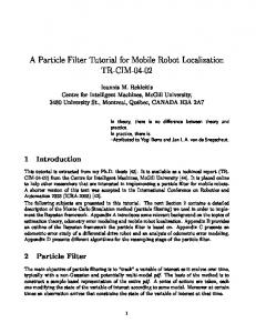
Number of non-empty cells after convergence

10000

8000

6000

4000

2000 m = 500 m = 1000 m = 2000

0 0

500 1000 1500 Number of non-empty cells after m samples

2000

Fig. 4: The function G for m = 500, 1000 and 2000. The x−axis represents ˜b, the number of bins filled after m samples have been generated. The y−axis plots b, the number of cells filled after convergence. Error bars indicate 95% confidence intervals for the b values, based on the training data. On many data points the intervals are too small to be visible.

of samples generated so far and ˜b is the number of bins filled by these samples. The function G can be learned beforehand from localization data. This data is obtained by performing multiple global localization runs using the adaptive particle filter on data sets collected in different environments. Figure 4 shows the function we have learned for three different values of m. Armed with G, we can now estimate the number of required samples for adaptive real-time particle filters. As we generate samples for the first sample set within a window, we update the number of non-empty cells ˜b based on the first m samples. G(m, ˜b) gives us b, the expected number of non-empty cells after convergence. Using b, Equation (3) gives us the number N of samples required to accurately represent the current belief. Whenever a new observation arrives, we generate a new sample set within the estimation window until the total number of samples reaches N . Hence small number of samples result in short estimation windows. Once enough independent samples are generated, the estimation window is finished, the approach determines the weights for the different sample sets within the window, and starts a new estimation window. Note that the computational overhead of this procedure is negligible (≈ 1%). IV. E XPERIMENTS We evaluated the effectiveness of our new approach, called ARTPF, against the alternatives using data collected from a mobile robot in a real-world environment. The task of the robot was to determine its position within the map in Figure 1, using data collected when moving around the loop on the left. To test the algorithms under extreme conditions, the robot moved approximately 70cm between each observation, and we only used data collected by two laser-beams, one pointing to the robot’s left, the other pointing to its right. Thus, localization was only based on the distance to the walls on the robot’s left

and right (see [6] for details on our sensor model). Note that the loop in the environment is symmetric except for a few “landmarks” along the walls of the corridor. Localization performance was measured by the average distance between the samples and the reference robot positions, which were computed offline. In the experiments, our adaptive real-time algorithm, ARTPF, is compared to standard particle filters with skipping observations and fixed number of samples per update, called SkipData (Figure 2a), to adaptive particle filters with skipping observations (labeled Adaptive, [5]), and RTPF with fixed number of samples (Figure 3, [8]) 3 . The comparison is performed as follows. First, the sample set size is fixed to N = 20,000 which is sufficient for the robot to globally localize itself. We then vary the processing power, where each approach is given the same amount of processing power. For example, a processing power of 100% refers to the ability to update all 20,000 samples between two observations, and a processing power of 25% refers to the ability to update only a quarter of the required samples. For RTPF, lower processing power means larger estimation windows. For SkipData, on the other hand, 25% processing power results in skipping 3 observations during each integration. Adaptive corresponds to SkipData with varying number of skipped observations, and ARTPF is similar to RTPF with varying window sizes. Figure 5 shows the evolutions of average localization errors over time using processing powers of 25% and 12.5%. Both graphs additionally include a BaseLine error, which is the error resulting from 100% processing power. Fig. 5a) shows that at 25% processing power, ARTPF localizes the robot significantly faster than the other methods. Furthermore, the two adaptive approaches ARTPF and Adaptive converge to the same error level as the Baseline approach. This is due to the fact that, as soon as the robot is localized, the number of samples drops enough to allow both approaches to integrate all observations, i.e. window size one for ARTPF. SkipData and RTPF, on the other hand, cannot reduce the number of samples, thereby skipping 3 (SkipData) or mixing 4 (RTPF) observations even when the robot is localized. At processing power 12.5% (Fig. 5 b), the advantage of ARTPF becomes even more prominent. SkipData has to skip 7 observations and thus fails to localize the robot. RTPF is clearly superior to SkipData, but still fails to reach an acceptable error level. Adaptive skips too many observations in the beginning and thus converges very slowly. After 450 seconds of localization, however, Adaptive outperforms RTPF since Adaptive can decrease the sample set size, thereby achieving higher update 3 Sensor aggregation as shown in Fig. 2b) is not applicable to our sensor model, and the insufficient performance of the approach shown in Fig. 2c) has already been demonstrated in [8].

800

600

400

200

80

Baseline SkipData RTPF Adaptive ARTPF

1400 1200

Localization error reduction %

Baseline SkipData RTPF Adaptive ARTPF

Average Localization error [cm]

Average Localization error [cm]

1000

1000 800 600 400

50

100

150

200

250 300 Time [sec]

350

400

450

500

(a)

60 50 40 30 20

0

0 0

RTPF ARTPF Adaptive

10

200 0

70

0

200

400 600 Time [sec]

800

1000

50

(b)

40

30 20 % processing power

10

0

(c)

Fig. 5: Performance of the different algorithms for a) 25% and b) 12.5% processing powers. The x-axis represents time elapsed since the beginning of the localization experiment. The y-axis plots the localization error measured in average distance from the reference position. Each point is averaged over 20 runs, and error bars indicate 95% confidence intervals. Both figures include the performance achieved with 100% processing power as the “Baseline” graph. Note that the x- and y-scales in a) and b) are different. c) Error reduction over SkipData for the same range of processing powers.

rates. ARTPF clearly outperforms all other approaches by combining the advantages of real-time particle filters with adaptive sample sets. In the beginning, when the high uncertainty requires large sample sets, the error drops at the same rate as RTPF. After 150 seconds, however, the window size starts to decrease, thereby giving ARTPF a clear advantage over the other approaches. Figure 5c) summarizes the performance of the approaches for different processing powers. It plots the error reduction achieved by each approach, compared to the vanilla particle filter (SkipData). Error reduction is measured by averaging the relative differences in localization errors. For example, at 15% processing power, ARTPF reduces the error by 77%, which means on average its localization error is less than one quarter of SkipData. The results show that ARTPF is the best among the algorithms, followed by Adaptive in the 15-50% processing power range. Below this level, however, RTPF outperforms Adaptive due to its better ability to handle insufficient computational resources. Adaptive finally degenerates into SkipData since it skips too many observations at the beginning of localization and thus cannot focus the samples properly. V. C ONCLUSIONS In this paper we introduced adaptive real-time particle filters, a novel particle filter approach to dealing with limited computing resources. Our approach combines the advantages of dynamic sample set sizes with real-time particle filters. To implement adaptive sampling, we use a learned mapping to obtain an estimate of the number of required samples. We demonstrated empirically that our technique produces significant performance improvements for robot localization under computational limitations. We expect our approach to be most useful in situations in which the complexity of the distribution changes over time and in which the stream of sensor data contains sparse, highly informative sensor readings. Despite these encouraging results, our approach has several limitations that warrant future research. The current

method does not take the dependencies between adaptive sampling and mixture weighting into account, i.e. it does not consider the fact that extreme mixture weights reduce the number of independent samples in a mixture. In future work, we want to use our method to determine the maximum travel speed of a mobile robot. For example, a robot should move slowly if it is highly uncertain about its location, since the update rate of the particle filter is rather low. When tracking its location, however, it can move at high speeds due to small sample sets. VI. ACKNOWLEDGEMENTS This research is sponsored in part by the National Science Foundation (CAREER grant number 0093406) and by DARPA (MICA program). VII. REFERENCES [1] Y. Bar-Shalom, X.-R. Li, and T. Kirubarajan. Estimation with Applications to Tracking and Navigation. John Wiley, 2001. [2] T. M. Cover and J. A. Thomas. Elements of Information Theory. Wiley, 1991. [3] P. Del Moral and L. Miclo. Branching and interacting particle systems approximations of Feynman-Kac formulae with applications to non linear filtering. In Seminaire de Probabilites XXXIV, number 1729 in Lecture Notes in Mathematics. Springer-Verlag, 2000. [4] A. Doucet, N. de Freitas, and N. Gordon, editors. Sequential Monte Carlo in Practice. Springer-Verlag, New York, 2001. [5] D. Fox. KLD-sampling: Adaptive particle filters. In Advances in Neural Information Processing Systems 14, 2002. [6] D. Fox, S. Thrun, F. Dellaert, and W. Burgard. Particle filters for mobile robot localization. In Doucet et al. [4]. [7] P. Jensfelt, O. Wijk, D. Austin, and M. Andersson. Feature based condensation for mobile robot localization. In Proc. of the IEEE International Conference on Robotics & Automation, 2000. [8] C.T. Kwok, D. Fox, and M. Meil˘a. Real-time particle filters. In Advances in Neural Information Processing Systems 15, 2003. [9] S.I. Roumeliotis and G.A. Bekey. Bayesian estimation and Kalman filtering: A unified framework for mobile robot localization. In Proc. of the IEEE International Conference on Robotics & Automation, 2000.