Journal of the Astronautical Sciences. Vol. 48, No. 4, Oct.âDec., 2000, Pages 537â551. A publication of the. American Astronautical Society. AAS Publications ...
Adaptive Realization of Linear Closed Loop Tracking Dynamics in the Presence of Large System Model Errors Hanspeter Schaub , Maruthi R. Akella
and
John L. Junkins
Simulated Reprint from
Journal of the Astronautical Sciences Vol. 48, No. 4, Oct.–Dec., 2000, Pages 537–551 A publication of the American Astronautical Society AAS Publications Office P.O. Box 28130 San Diego, CA 92198
Journal of the Astronautical Sciences
Vol. 48, No. 4, Oct.–Dec., 2000, Pages 537–551
Adaptive Realization of Linear Closed Loop Tracking Dynamics in the Presence of Large System Model Errors Hanspeter Schaub∗, Maruthi R. Akella†
and
John L. Junkins‡
Abstract A novel adaptive feedback control approach for nonlinear mechanical systems is presented. The approach applies to nonlinear trajectory tracking and has the remarkable property that the tracking error dynamics asymptotically approach a specified linear PID response for the case where the external disturbances are constant. The methodology applies to a large class of nonlinear mechanical systems, however, it is illustrated for the case of nonlinear rigid body maneuvers subject to actuator saturation constraints and large uncertainty of the system mass and inertia properties. While the system mass or inertias are not identified in this approach, the external disturbances are accurately estimated if they are constant or slowly varying with respect to the adaptation rate. A benefit of this method is that it requires no apriori knowledge of the unknown system parameters or bounds thereof.
Introduction Linear control theory has been studied extensively. One of its major advantages is that it provides several methods to design feedback gains that satisfy system requirements such as overall performance and control bandwidth are satisfied. However, since most dynamical systems are nonlinear in the large, the linear closed loop performance is only valid for finite neighborhoods about which the states were linearized. For large, nonlinear motions this linear control often looses its performance and stability characteristics. Nonlinear control theory ideally allows for global stability claims to be made for a class of systems including the actual nonlinear system, not only the locally valid linear model. However, enforcing requirements such as system performance and control bandwidth are ∗
Post-Doctoral Research Associate, Aerospace Engineering Department, Texas A&M University, College Station TX 77843. † Postdoctoral Associate, Center for Systems Science, Yale University, New Haven, CT 06511. ‡ George Eppright Chair Professor of Aerospace Engineering, Aerospace Engineering Department, Texas A&M University, College Station TX 77843, Fellow AAS.
1
2
Schaub, Akella and Junkins
typically difficult to achieve, especially during the entire nonlinear motion. Also, modeling errors and disturbances require compensation and complicate the discussion of actual closedloop performance. This paper presents an adaptive parameter update law which is superimposed on a nonlinear, feedback linearizing control law. The goal is to guarantee asymptotic stability of the overall system while forcing the actual closed-loop dynamics to be of a desired PID form. This allows for standard linear design techniques to be employed when selecting the feedback gains, while actually asymptotically approaching the desired closed-loop error dynamics even in the presence of large system parameter uncertainty. Several adaptive methods have been developed to control systems with unknown parameters.1–7 However, many of these adaptive update laws require some a priori knowledge of the unknown parameters. The adaptive control law in this paper requires no such knowledge. The reason for this is that the desired closed-loop dynamics are chosen to be of a kinematic form devoid of any system parameters such as mass or inertias. Also, while many traditional adaptive laws guarantee overall stability, they do not guarantee a specific closed-loop performance. The underlying nonlinear feedback control law used in this study is inherently very robust with regards to parameter uncertainties as has been shown in Ref. 8 and 9. It achieves asymptotic tracking of a reference motion even with very crudely known mass and inertia matrix. The presented adaptive law builds on this robust feedback law to enforce the desired closed-loop performance without losing overall stability claims. Schaub et. al. presented the first version of this update law in Ref. 9 where a simple attitude regulator problem is studied. This paper expands that study to encompass the trajectory tracking problem and the translational-rotational coupling effects. The translation and rotation of a rigid body is controlled to follow a prescribed trajectory. The first section develops the feedback linearizing control laws for the translational and rotational motion. The rigid body rotation is described through the Modified Rodrigues Parameters (MRPs) which allows for remarkable simplifications of the nonlinear feedback law while avoiding the typical singularities associated with three-parameter attitude descriptions. The second section outlines an adaptive update law which guarantees that the desired linear closed-loop trajectory is tracked asymptotically. A Lypapunov function is used to guarantee that the desired closed-loop motion is achieved.
Linear Closed-Loop Dynamics This section presents feedback linearizing control laws which achieve the desired linear closed-loop dynamics if no modeling errors are present. In this ideal case, both the translational and rotational control laws are determined that force a rigid body to track a commanded reference trajectory asymptotically. Translational Motion Let the translational position of a body relative to an inertial reference frame be given by the vector R. The commanded trajectory which the body is to follow is given by Rc (t) ¨ c are assumed to be given or obtained through direct for which the derivative R˙ c and R differentiation. The position tracking error r is then defined as r = R − Rc
(1)
Adaptive Realization of Linear Closed Loop Tracking Dynamics
3
The translational equations of motion are given through Newton’s second law as ¨ = uT + F ∗ m∗ R e
(2)
where uT is the net control force vector acting on the body and m∗ and Fe∗ are the true system mass and external disturbance force respectively. A general notation adopted here is that all variables with a superscript “∗” are the true values of the unknown quantities, while the corresponding variables without the asterix are the current adaptive estimates of these quantities. We desire the translational closed loop dynamics to be of the linear PID form Z t rdt = 0 (3) r¨ + PT r˙ + KT r + KT i 0
Notice that the scalar constants in Eq. (3) are simply control gains, no system parameters appear in this equation. If this exact closed-loop response is achieved, then we are able to employ linear control techniques to find appropriate gains that satisfy other system constraints such as control bandwidth limitations. We will find, however, that the desired dynamics of Eq. (3) can be asymptotically approached even in the presence of model uncertainties. Using the r definition in Eq. (1), the translational PID condition in Eq. (3) is rewritten as the following inertial acceleration constraint Z t ¨ ¨ R − (Rc − PT r˙ − KT r − KT i rdt) = 0 (4) 0
Defining the commanded translational acceleration vector φT to be Z t ¨ φT = Rc − PT r˙ − KT r − KT i rdt
(5)
0
a sufficient condition for Eq. (3) to be satisfied is that ¨ = φT R
(6)
Substituting Eqs. (5) and (6) into the translational equations of motion in Eq. (2), we express the translational, feedback linearizing control vector u∗T as u∗T = m∗ φT − Fe∗
(7)
Note however that for the control law in Eq. (7) to be implemented exactly, perfect knowledge of the system states m∗ and Fe∗ are required. Rotational Motion Let ω be the body angular velocity vector, then Euler’s rotational equations of motion of a rigid body are given by ˜ [I]ω˙ = −[ω][I]ω + uR + τe∗ +
N X i=1
[ρ˜i ]Fi
(8)
4
Schaub, Akella and Junkins
where [I] is the inertia matrix, uR is the control torque vector and τe∗ is the true external torque vector. The tilde matrix operator acts like the vector cross product and is defined for any vector a ∈ 1, the MRP vector remains bounded within a unit sphere. Switching, using Eq. (11), when the σ 2 = 1 surface is penetrated also results in the corresponding MRPs always measuring the shortest rotational distance (less than π) back to the origin.11, 12 The MRP kinematic differential equations are10, 11, 13, 14 1 σ˙ = [B(σ)]ω 4 where the matrix [B] = [B(σ)] is conveniently expressed as10, 11 � � � ˜ + 2σσ T [B] = 1 − σ T σ I3×3 + 2 [σ]
(12)
(13)
˜ being defined in the sense of Eq. (9). Note that the with the skew-symmetric matrix [σ] inverse of [B] has the convenient and elegant algebraic expression12 [B]−1 =
1 (1 + σ 2 )2
[B]T
(14)
To track a commanded rotation, various reference frames must be introduced. Let N be the inertial frame and B be the body frame. The reference frame of the commanded rotation is denoted by C. The MRP vectors σ, σc and s describe parametrically the following relative frame orientations. σ
⇒
ˆ = [BN (σ)]{n} ˆ {b}
(15a)
σc
N −→ C
⇒ ⇒
ˆ {ˆ c} = [BN (σc )]{n} ˆ = [BN (s)]{ˆ {b} c}
(15b)
s
N −→ B
C −→ B
(15c)
Adaptive Realization of Linear Closed Loop Tracking Dynamics
5
The error vector δω between actual and commanded body angular velocities is given by the vector expression δω = ω − ωc
(16)
Since angular velocity vectors typically have their components taken in their different reference frames, to compute the column matrix δω with B frame components, the direction cosine matrix [BC] is used to map the C frame components of ωc into B frame components with the following matrix equation. δω = ω − [BC]ωc
(17)
The kinematic differential equations of σc and s are then given by 1 σ˙ c = [B(σc )]ωc 4 1 s˙ = [B(s)]δω 4
(18) (19)
Let’s assume that we desire the closed loop dynamics to have the following prescribed linear PID form Z t s¨ + PR s˙ + KR s + KRi sdt = 0 (20) 0
where PR , KR and KRi are the positive scalar velocity, position and integral feedback gains. Again, this differential equation only contains kinematic quantities and no system properties such as inertias or external torques are present. Linear control theory states that for any initial s and s˙ error vectors, the resulting motion is asymptotically stable and the rigid body will track the commanded rotation asymptotically. The process of finding the corresponding feedback control law that will yield closed loop dynamics of the form in Eq. (20) has been shown by Schaub et. al. in Ref. 9 for the regulator case where ωc = 0. The result in Ref. 9 is expanded here to incorporate the tracking problem and the translational/rotational coupling. Eq. (20) is thus written as Z s¨ + PR s˙ + KR s + KRi 0
t
1 sdt = [B](ω˙ − φR ) 4
(21)
where the commanded rotational acceleration vector φR is expressed as � � � � δω 2 4KR T ˜ − I3×3 s φR = [BC]ω˙ c − [ω][BC]ω c − PR δω − δωδω + 1 + s2 2 −1
Z
− 4KRi [B]
t
sdt (22) 0
To obtain Eq. (21), the MRP kinematic differential equation in Eq. (19) and its derivative are substituted into Eq. (20). After performing some lengthy algebra and making use of the identities in Eqs. (14) and (17), the right hand side of Eq. (21) is found.
6
Schaub, Akella and Junkins
For Eq. (20) to be true, we must set ω˙ = φR . Using the rotational equations of motion in Eq. (8) we find the true feedback linearizing control law u∗R to be u∗R
˜ = [ω][I]ω + [I]φR − τe∗ −
N X
[ρ˜i ]Fi
(23)
i=1
Since the inertia matrix, external torque vector and CM moment arms are later assumed to be unknown quantities, we rewrite Eq. (23) so that these terms appear linearly as u∗R = [L∗ ]g + [M ∗ ]φR − τe∗ −
N X
[Ψ∗i ]Fi
(24)
i=1
where the matrices [L∗ ], [M ∗ ] and [Ψ∗i ] are defined as 0 I23 −I23 0 I13 [L1 ] = −I13 I12 −I12 0 I13 I33 − I22 −I12 I12 I11 − I33 [L2 ] = −I23 I22 − I11 −I13 I23 � � . [L∗ ] ≡ L1 .. L2 , [M ∗ ] ≡ [I]
(25)
(26)
(27)
[Ψ∗i ] ≡ [ρ˜i ]
(28)
and the 6 × 1 vector g is defined as � �T g ≡ ω12 ω22 ω32 ω1 ω2 ω2 ω3 ω3 ω1
(29)
For the development of the adaptive update laws, it is convenient to write the control torque expression in (24) in a more compact form as in Ref. 9. For this purpose, we introduce the 3 × (10 + 3N ) matrix [Q∗ ] . . . . . [Q∗ ] = [L∗ .. M ∗ .. τe∗ .. Ψ∗1 .. · · · .. Ψ∗N ]
(30)
and the (10 + 3N ) × 1 vector x
g φR −1 x = −F 1 . ..
(31)
−F2 The true feedback linearizing control torque u∗R is now written compactly in the form u∗R = [Q∗ ]x
(32)
Note that x is computed only from parameters which are assumed to be known, such as ω, σ, Fi and the commanded trajectories.
Adaptive Realization of Linear Closed Loop Tracking Dynamics
7
Adaptive Model Update Laws While the commanded acceleration vectors φT and φR are kinematic quantities depending ˙ respectively, to compute the proper only on the tracking error state vectors (s, δω) and (r, r) linearizing control vectors uT and uR exactly, the system parameters must be known exactly. References 8 and 9 have shown that this type of feedback linearizing control is very robust with respect to system parameter modeling errors. However, the transient closed loop dynamics can differ drastically from what is prescribed. The following development for adaptive control laws is split up again into translational and rotational sections. Note that for this dynamical system, the rotational motion does not affect the translational motion. However, the CM is assumed to be unknown and translational motion may produce moments that affect the rotational motion. Translational Parameter Update Laws Since the true system mass and external force vector are unknown, we replace the translational control law in Eq. (7) with uT = mφT − Fe
(33)
where m(t) and Fe (t) are the respective adaptive estimates of the system mass and external force vector. The next step is to derive adaptive update laws for m and Fe while guaranteeing that uT in Eq. (7) causes the rigid body to track the commanded motion Rc (t) asymptotically and ensure that the actual closed-loop dynamics are of the linear PID form shown in Eq. (3). The actual closed-loop dynamics will not satisfy exactly the desired form in Eq. (3) since uT 6= u∗T . Using Eqs. (2) and (33), the true closed-loop dynamics due to the adaptive control law uT are given by Z t � 1 � r¨ + PT r˙ + KT r + KT i rdt = ∗ mφ ˜ T − F˜e (34) m 0 where the estimation errors m ˜ and F˜e are defined as m ˜ = m − m∗ F˜e = Fe − F ∗
(35) (36)
e
Let the reference vector rR (t) have the same initial conditions as r (i.e. rR (t0 ) = r(t0 ) ˙ 0 )) and satisfy the differential equation and r˙ R (t0 ) = r(t Z t r¨R + PT r˙ R + KT rR + KT i rR dt = 0 (37) 0
This vector rR (t) indicates what the actual position error vector r(t) should be at time t if these errors were indeed decaying according to the PID equation in Eq. (3). To obtain a measure of error of achieving this desired closed-loop performance, we define the 9 × 1 vector �T to be R t 0 (r − rR )dt �T = r − rR (38) r˙ − r˙ R
8
Schaub, Akella and Junkins
Using Eqs. (3), (34), (37) and (38), the differential equation of �T is expressed as 0 0 I3×3 0 0 0 I3×3 �T + 0 �˙ T = ξT −KT i I3×3 −KT I3×3 −PT I3×3 {z } | {z } | [AT ]
(39)
bT
with ξT defined as the closed-loop performance disturbance due to estimation errors. ξT =
1 (mφ ˜ T − F˜e ) m∗
(40)
We use a Lyapunov function VT to derive the system update laws and guarantee overall asymptotic stability. Let VT be defined as � 2 � m ˜ 1 ˜T ˜ T VT = �T [T ]�T + ΓT + F Fe (41) γm γFe e where the 9 × 9 matrix [T ] is a symmetric, positive definite matrix and ΓT , γm and γFe are positive scalar learning rates. Taking the derivative of VT we find � � m ˜ ˙ 1 ˜ T ˜˙ T T T T ˙ VT = �T ([AT ] [T ] + [T ][AT ])�T + 2bT [T ] �T + 2ΓT m ˜ + F Fe (42) γm γFe e Assuming both the system mass m∗ and external force Fe∗ are constant, then m ˜˙ = m ˙ and ˙ ˜ ˙ F e = Fe . More generally, if Fe is variable, then less tight stability results can be derived. Furthermore, since [AT ] is a stable matrix, Lyapunov’s stability theorem for linear systems states that for any symmetric, positive definite matrix [RT ], there exists a corresponding symmetric, positive definite matrix [T ] such that the following algebraic Lyapunov function is satisfied:15 [AT ]T [T ] + [T ][AT ] = −[RT ]
(43)
Using these identities and by partitioning the 9 × 9 matrix [T ] into three 9 × 3 submatrices [Ti ] � � .. .. [T ] = T1 . T2 . T3 (44) the Lyapunov rate V˙ T is written as � � �� � � ΓT ˙ 1 1 ΓT T T T T T ˜ ˙ m ˙ + Fe Fe − [T3 ] �T ∗ VT = −�T [RT ]� + 2 m ˜ φT [T3 ] �T ∗ + m γm γFe m
(45)
By choosing ΓT = 1/m∗ , we are able to obtain the following update laws which are independent of the unknown true system mass m∗ . m ˙ = −γm φTT [T3 ]T �T F˙e = γF [T3 ]T �T e
(46) (47)
Adaptive Realization of Linear Closed Loop Tracking Dynamics
9
Using Eqs. (46) and (47), the Lyapunov rate is expressed simply as V˙ T = −�TT [RT ]�TT
(48)
which is a negative definite quantity in terms of �T . Therefore the adaptive control law uT given in Eq. (33) is asymptotically stabilizing with regards to �T and will force the true closed-loop dynamics to asymptotically approach the desired PID form. However, we note that the errors m ˜ and F˜e are not present in V˙ T . While the mass model ¨ c → 0 and the external force F ∗ is constant as error m ˜ will not necessarily go to zero, if R e seen in the body frame, then the external force model error F˜e will go to zero. Since the system is asymptotically stable, we know that �T → 0 and that some steady-state condition will be achieved. At this steady-state, the control uTss must satisfy uTss = mss φTss − Fess = −Fe∗
(49)
¨ c → 0, Eq. (5) shows that φT → 0. This implies that Fess → F ∗ and that the Since R ss e external force vector is learned perfectly for this case. For slowly varying Fe∗ , as compared to F˙e in Eq. (47), we can expect the external disturbance model errors to remain small. Rotational Parameter Update Laws The goal of the following adaptive control law is to find learning laws for the inertia matrix quantities [L] and [M ], and if necessary, for the external torque vector Fe and CM moment arm [Ψi ], such that the actual closed loop dynamics asymptotically approaches the desired linear PID form. Since the true inertia matrix, external torque vector and CM moment arms are unknown, we write the adaptive control torque vector uR as uR = [Q]x
(50)
where the adaptive system estimates [Q] are defined in Eq. (30). The following development parallels the study done in Ref. 9 for the simpler regulator case without the coupling to the translational motion. For the current case, the [Q] matrix is augmented by the various [Ψi ] submatrices. Since each [Ψi ] actually only has to model a three-parameter vector ρi , this method introduces a highly redundant set of parameter to model the CM moment arms vectors. It is possible to reverse the CM moment arm cross product order in Eq. (23) to read [F˜e ]ρi and obtain a minimal parameterization of the CM moment arm. However, having this matrix product order reversed prohibits the unknown true inertia matrix to be canceled out of the adaptive update laws. Therefore this developed is performed with the more redundant [Ψi ] notation. ˜ to be Defining the model error [Q] ˜ = [Q] − [Q∗ ] [Q]
(51)
the true closed-loop dynamics are given by9 Z s¨ + PR s˙ + KR s + KRi 0
t
1 ˜ sdt = [B][I]−1 [Q]x 4
Let the vector sr be the solution of the differential equation Z t s¨r + PR s˙ r + KR sr + KRi sr dt = 0 0
(52)
(53)
10
Schaub, Akella and Junkins
˙ 0 ). Thus the trajectory sr (t) represents the desired where sr (t0 ) = s(t0 ) and s˙ r (t0 ) = s(t PID closed loop performance. Any deviations from this performance are only due to system ˜ Analogous to the translational case, let the augmented 9 × 1 vector �R model errors [Q]. express the difference between the actual tracking errors and the reference tracking errors. R t 0 (s − sr )dt �R = s − sr (54) s˙ − s˙ r Using Eq. (52) and (53), note that the differential equation of �R is given by 0 I3×3 0 0 0 0 I3×3 �R + 0 �˙ R = −KRi I3×3 −KR I3×3 −PR I3×3 ξR | {z } | {z } [AR ]
(55)
bR
with the vector ξR defined as 1 ˜ ξR = [B][I]−1 [Q]x 4
(56)
Let us define the following positive definite Lyapunov function VR around the desired reference performance sr (t). � � ˜ T [ΓR ][Q][γ] ˜ −1 (57) VR = �TR [S]�R + tr [Q] where [S] and [ΓR ] are positive definite learning rate matrices and [γ] is a diagonal matrix containing the various learning rates γi . Taking the derivative of VR and using Eq. (55) we find � � � −1 ˜ T [Γ][Q][γ] ˜˙ V˙ R = �TR [S][AR ] + [AR ]T [S] �R + 2�TR [S]bR + 2tr [Q] (58) Since [AR ] is a stable matrix, there exists a positive definite matrix [RR ] such that [S][AR ] + [AR ]T [S] = −[RR ] By partitioning the 9 × 9 matrix [S] into three 9 × 3 sub-matrices [Si ] � � .. .. [S] = S1 . S2 . S3 the Lyapunov rate V˙ R is shown in Ref. 9 to be of the form �� � � ˙ −1 T −1 T T 1 ˜ ˙ ˜ [I] [B] [S3 ]�R x + [ΓR ][Q][γ] VR = −�R [RR ]�R + 2tr [Q] 4
(59)
(60)
(61)
Assuming that the body frame components of the true external torque vector Fe∗ and the CM moment arms [Ψ∗i ] are constant, then ˜˙ = [Q] ˙ − [Q˙ ∗ ] = [Q] ˙ [Q]
(62)
Adaptive Realization of Linear Closed Loop Tracking Dynamics
11
Choosing [ΓR ] = [I]−1 , Eq. (61) leads to the simple adaptive update law ˙ = − 1 [B]T [S3 ]T �xT [γ] [Q] 4
(63)
Enforcing Eq. (63), the corresponding Lyapunov rate function V˙ R reduces to V˙ R = −�TR [RR ]�R
(64)
Since V˙ is Eq. (64) is negative definite in the tracking error vector �R , this closed-loop performance error will decay to zero asymptotically. The adaptive system parameter estimate ˜ are stable. Since the reference motion sr (t) is globally, asymptotically stable, errors [Q] having � → 0 implies that the actual closed loop dynamics are also globally, asymptotically stable. ˜ and [M ˜ ] won’t necessary go to zero. For The inertia matrix adaptive estimate errors [L] the simpler uncoupled regulator case in Ref. 9, the external torque vector τe∗ is learned perfectly if it is a constant vector. This is no longer the case for this coupled tracking problem.
Numerical Simulations A rigid spacecraft with initial attitude, angular velocity and position errors is to track a command translation Rc (t) and rotation σc (t). The desired closed-loop translational and rotational dynamics are to be of the linear PID forms shown in Eqs. (3) and (20). Since the transient adaptive controls may grow relatively large, the methodology developed in Ref. 16 is employed here to obtain an admissible control. Given a generic control vector u and a corresponding vector of control saturation limits umax , the saturated control torque vector is found through ( ui for |ui | ≤ umaxi (65) u si = umaxi · sign(ui ) for |ui | > umaxi To guarantee that the control vector errors remain within a bounded region, the control error vector δmax is introduced. If |ui | − umaxi > δmaxi during periods of saturation, then the corresponding i-th row of the control vector parameters are reset to zero. For example, for the rotational control torque vector uR , this corresponds to zeroing the i-th row of the [Q] matrix. For the translational torque this process cannot be directly implemented since the scalar parameter m affects all three torque axis. In this case only the Fei components are zeroed unless all three axis are saturated. The numerical simulation parameters are given in Table 1. The initial [L(t0 )] matrix is constructed out of the corresponding [M (t0 )] matrix elements using Eqs. (25) through (27). The uT control vector is decomposed into three individual Fi vectors such that each Fi contained the i-th body axis component of uT . The positive definite matrices [RT ] and [RR ] are both chosen to be 9×9 identity matrices. Solving the algebraic Lyapunov equations in Eq. (43) and (59) and extracting the third block column submatrices, the matrices [T3 ] and [S3 ] are found to be 25.00000 I3×3 [T3 ] = [S3 ] = 155.6914 I3×3 (66) 259.5690 I3×3
12
Schaub, Akella and Junkins
Table 1: Numerical Simulation Data
Parameter R(t0 ) ˙ 0) R(t Rc (t0 ) R˙ c (t) m∗ m(t0 ) KT i KT PT γm γFe Fe∗ Fe (t0 ) uTmax δ uT σ(t0 ) ω(t0 ) σc (t0 ) ωc (t) [I]
[M (t0 )] KRi KR PR γi γτe γΨi τe∗ τe (t0 ) ρ∗1 ρ∗2 ρ∗3 ρi (t0 ) uRmax δ uR
Value [2.0 − 2.0 1.0] [0.5 0.5 − 1.0] [0.0 0.0 0.0] [0.1 0.0 0.0] 30 5 0.002 0.1 0.6 0.5 0.03 [0.75 − 0.75 − 0.5] [0.0 0.0 0.0] [2.0 2.0 2.0] [15 15 15] [−0.3 − 0.4 0.2] [0.2 0.2 0.2] [0.0 0.0 0.0] [0.20 0.01 0.03] 30 10 5 10 20 3 5 3 15 5 0 0 0 5 0 0 0 5 0.002 0.1 0.6 1000 0.05 0.1 [0.6 0.3 − 0.3] [0.0 0.0 0.0] [0.5 0.1 − 0.1] [−0.1 0.3 0.1] [0.1 0.1 0.2] [0.0 0.0 0.0] [1.5 1.5 1.5] [30 30 30]
Units m m/s m m/s kg kg sec−3 sec−2 sec−1
N N N N rad/s rad/s kg-m2
kg-m2 sec−3 sec−2 sec−1
N-m N-m m m m m N-m N-m
Adaptive Realization of Linear Closed Loop Tracking Dynamics
13
100 100
10-1 10-2
10-1
10-3 10-4
10-2
10-5
No Model Errors No Adaptation Adaptation without Saturation Adaptation with Saturation
10-3
No Adaptation Adaption without Saturation Adaptation with Saturation
10-6 10-7 10-8
0
100
200
300
0
100
time [s]
(a) Tracking Error |r| (m)
6 5 4 3 2 1 0 -1 -2 -3 -4 -5
5 4
No Model Errors No Adaptation
2 1 0 -1 -2 -3 -4 0
50
300
(b) Performance Error |r − rR | (m)
6
3
200
time [s]
100
150
No Model Errors Adaptation witout Saturation Adaptation with Saturation
0
50
100
150
time [s]
time [s]
(c) Control Vector uT (N-m)
(d) Control Vector uT (N-m)
Figure 1: Translation Tracking Errors
The resulting simulation is illustrated in Figures 1 and 2. Figure 1 shows the relevant translational states. The tracking error vector magnitudes for various cases are shown in Figure 1(a). The ideal linear PID response is shown as a grey line. If the translational feedback control law is used without any adaptive updates to the system models, then the tracking error still decay to zero. This supports the inherent robustness of this type of nonlinear feedback control law as was demonstrated in Ref. 8 and 9. However, the more general performance doesn’t always resemble the desired PID system due to model errors and disturbances. Activating the adaptive updates causes the performance to rapidly approach the desired closed-loop dynamics. With the control bounds active the closed-loop performance tracking degrades somewhat, but still provides very good asymptotic results. This behavior is also illustrated in Figure 1(b) where the difference between r and rR is plotted on a logarithmic scale. As expected, the performance error clearly degrades when control saturation is added. However, it remains substantially better then the non-adaptive case. Figure 1(c) permits the comparison of the ideal control vector u∗T and uT without adaptation active. The ideal control actually requires a rather large initial torque due to the initial errors and feedback gains chosen. Due to the small initial system parameter estimates, the translational control vector without adaptation appears smaller and smoother. Figure 1(d) compares active adaptation cases where the control saturation bound is either
14
Schaub, Akella and Junkins
1.0 0.8
10-1
0.6 0.4 0.2
10-2
0.0 -0.2
No Model Errors No Adaptation Adaptation without Saturation Adaptation with Saturation Adaptation without CM Learning
10-3
-0.4
No Model Errors No Adaptation With Adaptation
-0.6 -0.8 -1.0 0
100
10-4
200
0
300
100
200
300
time [s]
time [s]
(b) MRP Tracking Error |s|
(a) MRP Attitude Vector σ
3.0 2.5
-1
10
2.0 10-2
No Model Errors No Adaptation
1.5 1.0
10-3
0.5 10-4
0.0
No Adaptation Adaptation without Saturation Adaptation with Saturation Adaptation without CM Learning
-5
10
10-6 0
100
-0.5 -1.0 -1.5
200
300
0
100
time [s]
200
time [s]
(c) Performance Error |s − sr |
(d) Control Vector uR (N-m)
4
No Model Errors Adaptation without Saturation Adaptation with Saturation
3 2 1 0 -1 -2 -3 0
10
20
30
40
time [s]
(e) Control Vector uR (N-m)
Figure 2: Rotational Tracking Errors
50
300
Adaptive Realization of Linear Closed Loop Tracking Dynamics
15
imposed or not. Without saturation bounds the control vector components grow rather large for short periods of time before asymptotically approaching the ideal torques. With saturation active, various control vector components become saturated for during the first 30 seconds of the simulation and then approach the ideal torques. Note that with the chosen δuT that control chattering is not an issue, although some tuning maybe required in a given application. The rotational motion is illustrated in Figure 2. In Figure 2(a),it is very evident that while the feedback control law without adaptation is successful in tracking the commanded rotation σc (t), the transient errors grow very large. Figure 2(b) shows the tracking error magnitudes for various cases. Without adaptation, the tracking errors are one to two orders of magnitude larger than the reference attitude σr (t). With adaptation turned on, they remain very close to the ideal errors σr . With control saturation active, the tracking is only slightly degraded relative to the unsaturated case. Note that the cases where the CM moment arm learning is turned off the resulting performance is still very good for the first portion of the simulation. As the tracking errors become small (less than 10−2 for this case) they start to decay at a slower rate than the reference σr . The reason for this is the highly redundant parameterization of the inertia matrix through the matrices [L] and [M ]. This provides the adaptive control law with sufficient freedom to adjust these inertia estimate matrices to partially compensate for the unknown CM terms. Depending on the problem, a good bit of numerical computation can be saved by not updating on the CM moment arms. Similar conclusions are made in Figure 2(c) where the performance difference between s and sr is shown. At one point the adaptation free case has a performance error vector magnitude close to 1, which indicates the rigid body being close to 180 degrees off the desired attitude. The control torque vector components for the adaptation free case are shown in Figure 2(d). Note that here the controls never reaches the saturation limit, but they take a long time to converge. For the adaptive cases the controls are shown in Figure 2(e). With saturation active, some control vector components are saturated at times. But in both the saturated and unsaturated cases the control torque rapidly approaches the ideal control. These simulations support the validity of the theoretical developments and the practicality of this approach.
Conclusions An adaptive method is presented to enforce linear closed-loop dynamics while tracking a commanded translational and rotational trajectory. The general methodology used is applicable to a large class of nonlinear dynamical systems. If the external disturbances are constant in the body frame, the adaptive law is shown to be globally asymptotically stabilizing. By having a prescribed nominal linear closed-loop tracking error dynamics, even for large nonlinear motions, the process of designing feedback gains that match other system requirements such as overall performance and control bandwidth, is greatly simplified. Choosing the MRPs as attitude coordinates, a nonsingular, minimal attitude description is achieved. Numerical studies show that switching between the two sets of MRPs to avoid singularities has minimal impact on the performance. The numerical study illustrates that excellent trajectory tracking is possible with this adaptive control law, even though the system parameters are essentially unknown. For the attitude control problem, the learning/adaptation rate is shown to be fast enough for a large number of applications. Further, the numerical simulations also illustrate the theoretical developments to impose control
16
Schaub, Akella and Junkins
saturation with this adaptive control law. The adaptive control law with saturation limits active is still able to achieve good tracking. Finally, this study further reiterates the good general robustness properties of the non-adaptive nonlinear feedback control law which underlies the presented adaptive control law. In all but extreme cases, the non-adaptive feedback law is still able to achieve asymptotic trajectory tracking. However, it’s closed-loop dynamics differ substantionally from the desired linear PID form for large initial parameter errors.
Acknowledgments We are pleased to acknowledge that support for this work was provided by Allen Moshfegh of the Office of Naval Research. Fruitful discussions with Rush D. Robinett and R. A. Paielli also contributed to our early thinking that led to this work.
References [1] NARENDRA, K. S. and ANNASWAMY, A. , Stable Adaptive Systems. Prentice Hall, 1989. [2] SASTRY, S. and BODSON, M. , Adaptive Control: Stability, Convergence and Robustness. Prentice Hall, 1989. [3] CRISTI, R. and BURL, J. , “Adaptive Eigenaxis Rotations,” Proceedings of the European Control Conference, 1993, pp. 243–247. [4] JUNKINS, J. L. , AKELLA, M. R. , and ROBINETT, R. D. , “Nonlinear Adaptive Control of Spacecraft Maneuvers,” Journal of Guidance, Control and Dynamics, Vol. 20, No. 6, 1997, pp. 1104–1110. [5] AHMED, J. , COPPOLA, V. T. , and BERNSTEIN, D. S. , “Adaptive Asymptotic Tracking of Spacecraft Attitude Motion with Inertia Matrix Identification,” Journal of Guidance, Navigation and Control, Vol. 21, No. 5, 1998, pp. 684–691. [6] ZENG, Y. and SINGH, N. S., “Dynamic Feedback Linearizing Attitude Control of Spacecraft with Uncertain Dynamics,” AIAA Guidance, Navigation and Control Conference, (Boston, MA), Aug. 10–12 1998. Paper No. 98-4228. [7] IOANNOU, P. A. and SUN, J. , Stable and Robust Adaptive Control. Upper Saddle River, NJ: Prentice Hall, 1995, pp. 85–134. [8] PAIELLI, R. A. and BACH, R. E. , “Attitude Control with Realization of Linear Error Dynamics,” Journal of Guidance, Control and Dynamics, Vol. 16, No. 1, Jan.–Feb. 1993, pp. 182–189. [9] SCHAUB, H. , AKELLA, M. , and JUNKINS, J. L. , “Adaptive Control of Nonlinear Attitude Motions Realizing Linear Closed Loop Dynamics,” IEEE Transactions on Automatic Control. submitted for Publication. [10] SHUSTER, M. D. , “A Survey of Attitude Representations,” Journal of the Astronautical Sciences, Vol. 41, No. 4, 1993, pp. 439–517.
Adaptive Realization of Linear Closed Loop Tracking Dynamics
17
[11] SCHAUB, H. and JUNKINS, J. L. , “Stereographic Orientation Parameters for Attitude Dynamics: A Generalization of the Rodrigues Parameters,” Journal of the Astronautical Sciences, Vol. 44, No. 1, Jan.–Mar. 1996, pp. 1–19. [12] SCHAUB, H. , Novel Coordinates for Nonlinear Multibody Motion with Applications to Spacecraft Dynamics and Control. PhD thesis, Texas A&M University, College Station, TX, May 1998. [13] MARANDI, S. R. and MODI, V. J. , “A Preferred Coordinate System and the Associated Orientation Representation in Attitude Dynamics,” Acta Astronautica, Vol. 15, No. 11, 1987, pp. 833–843. [14] TSIOTRAS, P. , “Stabilization and Optimality Results for the Attitude Control Problem,” Journal of Guidance, Control and Dynamics, Vol. 19, No. 4, 1996, pp. 772–779. [15] JUNKINS, J. L. and KIM, Y. , Introduction to Dynamics and Control of Flexible Structures. Washington D.C.: AIAA Education Series, 1993. [16] AKELLA, M. R. , JUNKINS, J. L. , and ROBINETT, R. D. , “Structured Model Reference Adaptive Control with Actuator Saturation Limits,” AIAA/AAS Astrodynamics Specialist Conference, (Boston, MA), Aug. 10–12 1998. Paper No. 98-4472.