Adaptive Refinement Based on Stress Recovery Technique
Recommend Documents
Addison-Wesley Series in. Computer Science. Addison-Wesley, 1989. 4] Linda Stals. Parallel Multigrid on Unstructured Grids using Adaptive Finite Element ...
Nov 12, 2017 - We developed a framework for a distributed-memory parallel computer that enables dynamic data management for adaptive mesh refinement ...
Feb 22, 2018 - Abstract. An adaptive mesh refinement method is proposed for finite volume framework. The novelty of the method resides in using a dual data ...
second invariant of the deviatoric strain-rate tensor over an element is nearly the ... body is deformed in plane strain compression at a nominal strain-rate of 5000 ...
The recovery process must take into account both the intra-grid data dependencies as well as the inter-grid dependencies
Please send all correspondence to: T. Meinders, University of Twente, Mechanical Engineering. Department, Po Box ... sheet metal forming processes for wrinkling prediction. However .... Press Ponts et Chaussees, 71-78, 1985. 8. K.W. Neale ...
efficiency of the procedure and the importance of mesh refinement in multi-physics problems. У 2005 Elsevier B.V. All rights reserved. Keywords: Porous media ...
Official Full-Text Publication: Component-Based Recovery Block Technique on ... In applications where computer systems are used to manage critical tasks, ...
ISBN 978-88-95608-23-5; ISSN 1974-9791. A New Technique for Heavy Oil Recovery Based on. Electromagnetic Heating: System Design and Numerical.
Electromagnetic Heating: Pilot Scale Experimental ... phenomena connected with the electromagnetic heating of an oil sand reservoir up to 150 °C, in order to.
enhanced oil recovery methods, such as thermal recovery. ... physical parameters measured on real oil sand samples and heating requirements relative to an ...
Clip1 (fish) and clip2 (ran) as test clips, each one of them is in size of ... CR which are resulted from applying of this method on clip1 and clip2, respectively. (a).
Mar 15, 2014 - Asking questions is a tool for many systems to achieve a specific goal including assessment and enhancing learners' ..... 13.58 ± 1.49. 8.58 ± ... Question Generation, The Tenth International Conference on Intelligent Tutoring ...
Abstract. Compressed bit streams are, in general, very sensitive to channel errors. For instance, a single bit error in
technique based on the modified Yule-Walker filter. Con- .... using a modified Yule-Walker (MYW) recursive filter. .... valuable comments from Thomas F. Quatieri.
using Least Square Support Vector Method (LS-SVM) for liquid level measurement using Capacitance Level Sensor. (CLS) is reported in this paper.
Mar 28, 2016 - Abstract. Disaster recovery and business continuity plans are essential to make sure businesses keep on going. However, many small and ...
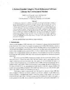
Robust Parallel Adaptive Mesh Refinement Software. Library for Unstructured Meshes. John Z. Lou, Charlcs D. Norton, and Tom Cwik. Jet Propulsion Laboratory.
for Soft Goal Elicitation for the development of an Web. Based News Application. We present an ... and prepares a SRS for software development. Requirements ...
middle ground to combine accuracy and adaptability. â A spectral element code, the Geophysical-astrophysical spectral-element adaptive refinement (GASpAR) ...
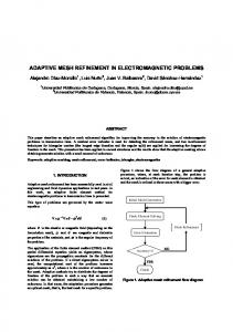
This paper describes an adaptive mesh refinement algorithm for improving the accuracy in the solution of electromagnetic problems in transmission lines.
Klotz 19], L ohner et al 24], Marcum et al 25], Powell and Ashford 29]). Re ning by adding grid points to a unique mesh is actually well-adapted to unstructured ...
refinement creates new elements the load quickly becomes unbalanced and so .... Warren and Salmon 5, 6] use a 3-dimensional Morton order key for N-body ...
Nov 6, 2002 - A special numerical multilevel technique associated with a particular hierarchical data structure is adaptive mesh refinement (AMR). This.
Adaptive Refinement Based on Stress Recovery Technique
Jun 28, 2017 - Introduction. The error assessment tools used in finite element analysis are well known and ... Mathematical Problems in Engineering. Volume 2017 ... the kriging interpolation in mesh-free methods in order to compare with ...... 227â234, 2009. [24] C. D. Lloyd and P. M. Atkinson, âAssessing uncertainty in.
Hindawi Mathematical Problems in Engineering Volume 2017, Article ID 1790256, 10 pages https://doi.org/10.1155/2017/1790256
Research Article 𝑝-Adaptive Refinement Based on Stress Recovery Technique Considering Ordinary Kriging Interpolation in L-Shaped Domain Kwang S. Woo1 and Jae S. Ahn2 1
Department of Civil Engineering, Yeungnam University, 280 Daehak-Ro, Gyeongsan, Gyeongbuk 38541, Republic of Korea School of General Education, Yeungnam University, 280 Daehak-Ro, Gyeongsan, Gyeongbuk 38541, Republic of Korea
1. Introduction The error assessment tools used in finite element analysis are well known and usually classified into two strategies: recovery-based error estimators and residual-type estimators [1, 2]. Stress recovery procedures can be classified as local (i.e., element level), patch-based, and global. To obtain a smooth stress field, averaging either projected or consistent finite element nodal stresses is an example of a patch-based scheme. The ideas of Zienkiewicz and Zhu [3–5] using the superconvergent patch recovery (SPR) are often preferred by researchers since they are robust and simple to use. Some references [6–11] contain extensive reviews of the different proposals for improving the SPR technique. They used the conventional LSM (least square method) to obtain recovered stresses from the ℎ-version of finite element solution at the sampling quadrature points. However, the residual-type error estimators have been proposed to evaluate errors for highorder hierarchical elements [12–14]. The residual error for
high-order hierarchical elements is the difference between the displacement fields over the original and a refined mesh and is computationally more expensive than the 𝑍/𝑍 (Zienkiewicz and Zhu) error estimate. Recently, some researchers [6, 7] used a weighted superconvergent patch recovery technique in which the recovered stresses are calculated by using weighting parameters. In addition to these, the recover-based technique has been also extended to mesh based PUMs and the X-FEM (extended finite element method) [15]. Rodenas et al. [16] also explored the capabilities of a recovery technique based on an MLS (moving least squares) fitting, more flexible than SPR techniques as it directly provides continuous interpolated fields without relying on an FE mesh, to obtain estimates or the error in energy norm as an alternative to SPR. In the context of FEM model, the kriging interpolation technique has been employed as an alternative for estimating the derivative of the unknown variable at any point of interest [17]. This method uses a variogram to express the spatial correlation,
2
Mathematical Problems in Engineering
and it minimizes the error of predicted values. It estimates the value at a location of interest as a weighted sum of data values at surrounding locations. The weight factors are assigned according to the variogram function that gives a decreasing weight with increasing distance between the given location and one of the surrounding locations. Dai [18] used the kriging interpolation in mesh-free methods in order to compare with the radial point interpolation method (RPIM) based on local supported radial basis function (RBF) and the Galerkin weak form. The literature on kriging interpolation for FEM, however, is very limited [14]. The 𝑝-adaptive finite element analysis based on the error estimation consists of two stages: a posteriori error estimation and the automatic mesh refinement. The goal is to increase the 𝑝-level nonuniformly so that the error is within the specified tolerance. The estimated errors in the finite element solution are of primary importance because of the basis for adaptive mesh refinement [19–21]. To minimize the computational cost, an effective and reliable technique of postprocessing is necessary for use in adaptive mesh refinement. It is known that the 𝑍/𝑍 error estimate has not been directly extended to the 𝑝-refinement [12, 13, 22, 23] because the high-order shape functions used to interpolate displacements within an element are also used to interpolate recovered stresses. The objective of this study is to demonstrate the applicability of OK (ordinary kriging) interpolation to the 𝑝adaptive refinement of L-shaped domain problem employing the modified SPR method for stress recovery. To verify this method, the limit value approach is proposed to predict the exact strain energy for nonsmooth problems based on the application of the equation of a prior error indicator in the asymptotic range to three FEMs with three successively higher levels of polynomial approximation.
ℎ
Δℎ
Δℎ
Known data points
Figure 1: Definition of the allowable limit of separation distance.
(ℎ) C0
a Linear variogram Spherical variogram Exponential variogram
ℎ Gaussian variogram Experimental variogram
Figure 2: Comparative plot of theoretical semivariogram models.
2. Ordinary Kriging Interpolation The OK method is a geostatistical interpolation technique that requires both the distance and the degree of variation between known sampled data points when estimating values at unsampled locations, in other words, firstly, to calculate the distances between the predicted unknown point and the measured points nearby and, secondly, to derive the weight of each of these surrounding measured points by using the value of the variogram against those distances. The derived weights at unknown points result in optimal and unbiased estimates by minimizing the error variance. 𝛾(ℎ) defined in (1) is often called a semivariogram or semivariance that can be defined as half the expected squared difference between paired random functions 𝑆(𝑥𝑖 ) denoted by stresses in FEM, separated by the distance and direction vector called by lag or separation distance ℎ [24, 25] such as 𝛾 (ℎ) =
1 𝑛 2 ∑ [𝑆 (𝑥𝑖 ) − 𝑆 (𝑥𝑖 + ℎ)] , 2𝑛 𝑖=1
(1)
where 𝑛 is the number of pairs of values of which the separation distance is marked with ℎ. When the semivariance is plotted against the lag distance or separation distance
between points, the plot is called semivariogram. For any given set of spatial data 𝑆(𝑥𝑖 + ℎ) separated from 𝑆(𝑥𝑖 ), there will generally be at most one pair that are separated by a given distance ℎ. However, the observed data may be scattered near the separation distance ℎ. One must necessarily aggregate point pairs [𝑆(𝑥𝑖 ), 𝑆(𝑥𝑖 + ℎ)] with similar distances ℎ ± Δℎ where Δℎ is called the allowable limit of separation distance as shown in Figure 1. Thus the separation distance ℎ can be allowed to use the similar distance denoted by ℎ ± Δℎ. Sample data belonging to a certain interval ℎ±Δℎ are averaged to find the representative value at a given distance ℎ. The semivariogram model is a function of three parameters, known as the nugget effect, sill, and range. Theoretically, at zero separation distance, the semivariogram value should be zero. However, at an infinitesimally small separation distance, the difference between measurements often does not tend to zero. This is called the nugget effect. Thus, the theoretical semivariogram model with a nugget effect can be fitted where the sill denoted by 𝐶0 means the maximum semivariogram value that is the plateau of Figure 2. As the separation distance of two pairs increase, the semivariogram
Mathematical Problems in Engineering
3 Equation (7) can be rewritten as
Table 1: Different models of variograms. Model Linear
If variance and covariance in the above equations are marked as below 𝜎2 = var (𝑠0 ) ;
(9)
𝜎𝑖𝑗2 = cov (𝑠𝑖 , 𝑠𝑗 ) of those two pairs also increases. Eventually, the increase of the separation distance cannot cause the semivariogram increase. The separation distance when the semivariogram reaches plateau is called range 𝑎. The example of schematic variogram graphs has been plotted in Figure 2 with respect to different variogram models. Several theoretical kriging modules are shown in Table 1. As mentioned earlier, the OK estimates are linear weighted moving average of available observations or Gauss points in the FEM [23, 24] 𝑛
The error variance associated with the OK estimate is called the minimum variance unbiased estimator or best linear unbiased estimator, since the constraint condition defined in (3) should be applied to minimize the variance of estimate errors. Based on the method of Lagrange multipliers, the mathematical form considering (3) and (10) can be expressed as
𝑖=1
where 𝜆 𝑖 and 𝑆(𝑥𝑖 ) are the weights assigned to the available observations and neighbor data close to the unsampled location 𝑥0 , respectively. The weight factors add up to unity to ensure that the estimate is unbiased.
𝑛
𝑖=1 𝑗=1
When a calculated stress value at any point is 𝑠0 and the corresponding true value is 𝑠0∗ , an error variance based on OK technique is as follows: 2
where 𝐿(𝜆 1 , 𝜆 2 , . . . , 𝜆 𝑛 , 𝜇) is a Lagrange objective function and 𝜇 is a Lagrange multiplier. In addition, number 2 in the fourth term in (11) is used to derive final equations with simple form. Minimizing the objective function can be carried out by finding the partial derivatives with respect to 𝜆 𝑙 (𝑙 = 1, 2, . . . , 𝑛) and 𝜇 such that
Equation (4) can be written as below 2 𝜎OK = var (𝑠0 ) + var (𝑠0∗ ) − 2 cov (𝑠0 , 𝑠0∗ ) .
In this work, the higher-order approximation based on Lobatto shape functions [26] which is often called integrals of Legendre polynomials [14, 23] with hierarchical properties is adopted to obtain displacements as a result of FEM. The SPR technique proposed by Zienkiewicz and Zhu [3, 5] has been adopted after a suitable modification to be compatible with the adaptive p-refinement procedure since the number of sampling Gauss points in each element is increased as the 𝑝-level becomes higher. The increment of the quadrature point has an effect on the stress norm. According to 𝑍/𝑍, ‖𝑒𝑟 ‖ represents the local error for a particular element, measured in energy norm. 𝜎∗ is the recovered stress resultant field or estimated exact stress field over the patch of elements (normally consisting of 4 elements) surrounding the patch node. The estimated exact stress field denoted by 𝜎∗ is determined by using the ordinary kriging interpolation technique. A posteriori error estimate in a particular energy norm is computed by summing its elemental contribution as
3. A 𝑝-Adaptive Refinement Using Modified SPR Technique Adaptive procedures are to implement iteration analysis based on distinctly different levels of space (ℎ)- or function (𝑝)-refinements in specified local region to achieve solutions having a certain degree of accuracy in an optimal fashion. Particularly the 𝑝-adaptive refinement makes it easy to use the initial meshes kept unchanged with selective increase in the polynomial order of shape function that is called “selective or nonuniform 𝑝-refinement” in FEM. The continuity between meshes with different polynomial order is achieved by assigning zero to the higher-order derivatives associated with edges in common with the lower derivatives. Thus, the higher-order of approximation is degraded to the lower along the interelement boundary. For this purpose, two important algorithms should be established such as an automatic 𝑝adaptive mesh refinement scheme and a posteriori error estimator for 𝑝-refinement strategy.
where 𝑆∗ is a column vector including the true stresses; 𝑆𝑝 including the stresses interpolated by Lobatto shape functions with the displacements obtained by FEM; [𝐷] is a constitutive matrix; Ω is a mesh domain. Here a smoothed continuous stress concept is applied for the true stresses 𝑆∗ that are obtained by the aforementioned OK technique. For the proposed technique, the weight factors depending on the distance between a sampling point and the point corresponding to an unknown value are considered. On the other hand, no weight factor is used in the original SPR technique based on LSM. The energy norm of the stress field itself may also be expressed in terms of stresses as follows: 𝑇
‖̂𝑟‖ = (∫ (𝑍𝑝 ) [𝐷]−1 𝑍𝑝 𝑑Ω) Ω
1/2
.
(17)
Thus, the relative percentage error can be defined as 1/2 2 𝑒 𝜂Ω = ( 2 𝑟 2 ) . 𝑒𝑟 + ‖̂𝑟‖
(18)
In case of the modified SPR method using ordinary kriging, however, the estimated exact stress field denoted by 𝑆∗ should be calculated at each iteration round of 𝑝refinement. In other words, 𝑆∗ cannot be fixed in the whole process of 𝑝-adaptive refinement the same as ℎ-adaptive refinement since this process is based on a posteriori error estimate. Thus, a new error estimator is proposed on the basis of a prior error estimator to verify the modified SPR method. The limit value approach is proposed to predict the exact strain energy for nonsmooth problems based on the application of the equation of a prior error indicator in the asymptotic range to three FEMs with three successively
Mathematical Problems in Engineering
5 Y2
Computational domain a a
Y2
a
Element 1
Element 2
Y1 y
a
X1
x
X2
Y1 Element 3
X1
X2
(b) Finite element mesh by 𝑝-FEM
(a) L-shaped domain
Figure 3: Plate with a square cutout.
higher levels of polynomial approximation. In the presence of singularities, the asymptotic convergence behavior of the 𝑝-version of the FEM permits a close estimate of the exact strain energy by extrapolation that is called the limit value, and hence we can predict the error in the energy norm on the finite element mesh employed. For a two-dimensional problem, under the assumption that the error in the energy norm has entered the asymptotic range where 𝑈ex and 𝑈fe are the strain energy, the rate of convergence for the p-version of FEM can be derived by the inverse theorem [23, 27] as 𝑘 𝑈ex − 𝑈fe ≤ 2𝛼 , 𝑁𝑝
(19)
where 𝑈ex and 𝑈fe are the exact strain energy estimated by the limit value and the approximate strain energy by FEM, 𝛼 is the strength of singularity, and 𝑁𝑝 and 𝑘 are the degrees of freedom for the polynomial order 𝑝 and a constant which depends on the mesh, respectively. There are three unknowns 𝑈ex , 𝑘, and 𝛼 in (19). By performing three successive extension processes, 𝑝−2, 𝑝−1, and 𝑝, which are in the asymptotic range, we have three equations for computing the unknowns. Cancelling 𝛼 and 𝑘 in (19), the following extrapolation equation can be derived as 𝐿 𝐿 − 𝑈𝑝 ) / (𝑈ex − 𝑈𝑝−1 )) log ((𝑈ex 𝐿 −𝑈 𝐿 log ((𝑈ex 𝑝−1 ) / (𝑈ex − 𝑈𝑝−2 ))
=
log (𝑁𝑝−1 /𝑁𝑝 ) log (𝑁𝑝−2 /𝑁𝑝−1 )
(20)
,
where 𝑈𝑝 , 𝑈𝑝−1 , and 𝑈𝑝−2 are the strain energies when the 𝐿 represents polynomial orders are 𝑝, 𝑝 − 1, and 𝑝 − 2 and 𝑈ex the limit value in terms of estimated exact strain energy where 𝑁𝑝 , 𝑁𝑝−1 , and 𝑁𝑝−2 are the number of degrees of freedom for each analysis. Computational experiences show this estimated limit value to be reliable and accurate for twodimensional elastostatic problems, especially in the presence
of singularity [14, 23] which give no exact solution. Thus, the percentage relative error expressed by energy norm using limit value is defined by (21). It is noted that (21) is not used for local indicator in practice but is used only to validate whether the modified SPR technique is reliable and accurate. If the local error estimate ‖𝑒𝑟 ‖ in (16) is large, the polynomial order should be increased to satisfy an acceptable level of accuracy 𝜌Ω = [
𝐿 − 𝑈𝑝 𝑈ex 𝐿 𝑈ex
1/2
]
,
(21)
𝐿 is the exact global strain energy and 𝑈𝑝 is also where 𝑈ex the global strain energy calculated in the current 𝑝-adaptive mesh consisting of nonuniform 𝑝-distribution at a certain iteration number.
4. Numerical Analysis The numerical example is shown in Figure 3 that specifies the geometric definition and analysis conditions that are given by 𝑎 = 50 cm, 𝑡 = 1.0 cm, 𝐸 = 2 × 10⁷ N/cm2 , ] = 0.3, and 𝜎 = 10 N/cm2 . Due to the symmetry, a quarter of plate is modeled by three elements with fourth-degree polynomials for shape functions of 𝑝-version finite element analysis. Figure 4 shows a 3D stem plot for distribution of von-Mises stresses at Gauss points. The stress values obtained from finite element analysis are considered as raw data for stress smoothing. In Figure 5, the experimental semivariogram has been plotted with respect to the separation distance ℎ. The allowable limit of separation distance Δℎ is assumed by 25% of ℎ. Thus, the separation distance ℎ can be allowed to use the similar distance denoted by ℎ ± Δℎ. Based on experimental semivariogram, three different theoretical semivariogram modules as shown in Table 1 have been tested. In this study, the Gauss model with Δℎ = 25% of ℎ has been adopted to find the weight factor for the OK process explained in (2). Before the further analysis of 𝑝-adaptive refinement, the performance between LSM and OK method is compared
6
Mathematical Problems in Engineering Table 2: The relative percentage errors of 12-element model by the modified SPR method.
Stresses (N/cG2 )
50
Number of iterations 25
Y2 Y1
X2 X1
Figure 4: Raw data from 𝑝-FEM analysis when 𝑝-level = 4.
Table 3: The relative percentage errors of 12-element model by the limit value.
0.25
Variogram
1 2 3 4 5 6 7 8 9 10
Least square method
0
1
2
3
4
5
Distance Experimental Gaussian
Spherical Polynomial
Figure 5: Comparison of semivariogram models using Δℎ/ℎ = 0.25 when 𝑝-level = 4.
with each other in Figures 6 and 7. As described earlier, the FEM raw data represents the computed von-Mises stress at Gauss points obtained by the 𝑝-version finite element model in Figure 3. Due to the discontinuity of stresses along the element interboundary, it is seen that the stress distribution is not smooth as shown in Figure 6(a). Thus, the stress recovery techniques are applied for stress smoothing. One is LSM based on equal weighted interpolation and the other is OK method by weighted interpolation using variogram model. It is noted that the corner singularity denoted by von-Mises stress is well expressed by OK interpolation comparing with LSM that are shown in Figures 6(b), 6(c), 7(b), and 7(c). To illustrate the applicability of OK interpolation to the 𝑝-adaptive mesh refinement, two 𝑝-version models are considered by 3-element and 12-element model. The initial 𝑝-level of both models begins with one. For nonuniform 𝑝distribution, the continuity between elements with different polynomial orders is achieved by assigning zero higher-order derivatives associated with the edge in common with the lower-order derivatives. The iteration step for 𝑝-adaptivity
is proceeded to final adaptive mesh based on a posteriori error estimation. In this study, the modified SPR technique is proposed to estimate the smoothed stress field by projection that is considered as an exact solution to calculate a posteriori error. The final adaptive mesh is automatically determined by the developed computer program for the purpose that are shown in Figures 8 and 9. The relative percentage errors have been illustrated in Tables 2 and 3 according to iteration numbers by using the modified SPR method as well as the limit value approach. The first error estimator by the modified SPR method is the objective of this study considering a posteriori error estimator as shown in Table 2. However, the relative percentage errors are not converged gradually, especially when higher-order polynomials are used in the 𝑝-adaptive mesh regardless of least square method or OK interpolation since the estimated exact stress field can be reproduced at each iteration round. To verify the proposed error estimator, the limit value approach based on a prior error estimate is used to evaluate the relative percentage error in Table 3. Since the exact strain energy is fixed as a certain value, the relative percentage errors are gradually decreased. As shown in Tables 2 and 3, the required number of iterations to determine the final adaptive
Mathematical Problems in Engineering (N/cG2 ) 5
Y2
7 (N/cG2 )
Y2
5
10 15 20 25
Y1
30
Y1
45
10
15
15 20
Y1
25
30
30
35
35
40
40 45
45
X1
(a) Raw data
10
25
40
X2
5
20
35
X1
(N/cG2 )
Y2
X2
X1
(b) OK interpolation
X2
(c) LSM
50
50
40
40
30
Stresses (N/cG2 )
Stresses (N/cG2 )
Figure 6: Stress contours by different interpolation techniques when 𝑝-level = 4.
Y2
20 10
X2
0
30
Y2
20 10
X2
0
(a) Raw data
(b) OK interpolation
Stresses (N/cG2 )
50 40 Y 2 30 20 X2
10 0
(c) LSM
Figure 7: Stress plots by different interpolation techniques when 𝑝-level = 4.
mesh is 10 by the LSM based 𝑝-adaptive model and 8 by OK based p-adaptive model. From this result, it is observed that the OK interpolation technique is more suitable for adaptivity procedures than the LSM that has been commonly used in the FE analysis.
In the case of LSM with NDF = 363, the relative percentage error shows 5.48%, but OK yields 4.17% when NDF = 353 as shown in Table 2. However, the relative percentage error based on the limit value is 5.78% for LSM and 5.61% for OK, respectively, as shown in Table 3. It is observed that
8
Mathematical Problems in Engineering
8
7
7
Relative percentage error (%)
40 6
8
8
(a) OK interpolation
(b) LSM
Figure 8: The final 𝑝-adaptive meshes by 3-element model.
30
20
10
0
0
50
100
150
200
Number of degrees of freedom
7
5
5
3
5
5
5
Least square Kriging
3
(a) 3-element model
7
6
4
8
4
4
3
7
5
5
5
8
5
5
(a) OK interpolation
40
6
(b) LSM
Figure 9: The final 𝑝-adaptive meshes by 12-element model.
Relative percentage error (%)
3
30
20
10
0
0.0078
0
100
200
300
400
Strain energy (N·m)
Number of degrees of freedom Least square Kriging
0.00778 p=8
(b) 12-element model
0.00776
p=7 p=6
Figure 11: Convergence characteristics of 𝑝-adaptive model using modified SPR method.
0.00774
0.00772
0
1
2
3
1000/NDF
Figure 10: Estimation of exact strain energy by limit value approach.
proposed 𝑝-adaptive models are plotted in Figures 11-12. It is noted that stable convergence pattern by the limit value approach is shown without any numerical oscillations, unlike the modified SPR method.
5. Conclusions the exact strain energy can be found by 𝑈ex = 7.7788 × 10⁻³ from Figure 10 that has been used to estimate the relative percentage error at each iteration round. In other words, in 𝐿 is the exact global strain energy, and 𝑈𝑝 is the global (21), 𝑈ex strain energy calculated in the current 𝑝-adaptive mesh consisting of nonuniform 𝑝-distribution at a certain iteration round. Thus, (21) cannot be used for local indicator in practice but is only used to check whether the modified SPR method is reliable and accurate. The convergence characteristics of
The new 𝑝-adaptive finite element model with the OK interpolation technique is proposed in this study. This approach shows better performance to determine the final adaptive mesh than the existing SPR method by 𝑍/𝑍 using LSM to estimated exact stress field by projection. This proposed model is very suitable for stress singularity problems since the higher weight factor is used to interpolate the calculated stresses at the Gauss points near stress singular points by applying theoretical variogram model and OK interpolation. In addition, the proposed new error estimator based on limit
Mathematical Problems in Engineering
9
Relative percentage error (%)
50 40 30 20 10 0
0
50
100
150
200
250
Number of degrees of freedom Least square Kriging
(a) 3-element model
Relative percentage error (%)
40
30
20
10
0
0
100
200
300
400
Number of degrees of freedom Least square Kriging
(b) 12-element model
Figure 12: Convergence characteristics of 𝑝-adaptive model using limit value approach.
value using exact strain energy can be used to a prior error estimate.
Conflicts of Interest The authors declare that there are no conflicts of interest regarding the publication of the paper.
Acknowledgments This work was supported by the 2015 Yeungnam University Research Grant.
References [1] M. Ainsworth and J. T. Oden, A Posteriori Error Estimation in Finite Element Analysis, John Wiley & Sons, New York, NY, USA, 2011.
[2] A. A. Yazdani, H. R. Riggs, and A. Tessler, “Stress recovery and error estimation for shell structures,” International Journal for Numerical Methods in Engineering, vol. 47, no. 11, pp. 1825–1840, 2000. [3] O. C. Zienkiewicz and J. Z. Zhu, “A simple error estimator and adaptive procedure for practical engineering analysis,” International Journal for Numerical Methods in Engineering, vol. 24, no. 2, pp. 337–357, 1987. [4] O. C. Zienkiewicz and J. Z. Zhu, “The superconvergent patch recovery and a posteriori error estimates. Part 1: the recovery technique,” International Journal for Numerical Methods in Engineering, vol. 33, no. 7, pp. 1331–1364, 1992. [5] O. C. Zienkiewicz and J. Z. Zhu, “The superconvergent patch recovery and a posteriori error estimates. Part 2: error estimates and adaptivity,” International Journal for Numerical Methods in Engineering, vol. 33, no. 7, pp. 1365–1382, 1992. [6] A. R. Khoei, H. Moslemi, K. M. Ardakany, O. R. Barani, and H. Azadi, “Modeling of cohesive crack growth using an adaptive mesh refinement via the modified-SPR technique,” International Journal of Fracture, vol. 159, no. 1, pp. 21–41, 2009. [7] A. R. Khoei, M. Eghbalian, H. Moslemi, and H. Azadi, “Crack growth modeling via 3D automatic adaptive mesh refinement based on modified-SPR technique,” Applied Mathematical Modelling, vol. 37, no. 1, pp. 357–383, 2013. [8] Q. Z. Xiao and B. L. Karihaloo, “Improving the accuracy of XFEM crack tip fields using higher order quadrature and statically admissible stress recovery,” International Journal for Numerical Methods in Engineering, vol. 66, no. 9, pp. 1378–1410, 2006. [9] B. Boroomand and O. C. Zienkiewicz, “An improved REP recovery and the effectivity robustness test,” International Journal for Numerical Methods in Engineering, vol. 40, no. 17, pp. 3247–3277, 1997. [10] B. Boroomand and O. C. Zienkiewicz, “Recovery by equilibrium in patches (REP),” International Journal for Numerical Methods in Engineering, vol. 40, no. 1, pp. 137–164, 1997. [11] N.-E. Wiberg and F. Abdulwahab, “Patch recovery based on superconvergent derivatives and equilibrium,” International Journal for Numerical Methods in Engineering, vol. 36, no. 16, pp. 2703–2724, 1993. [12] D. Kelly, D. S. Gago, O. Zienkiewicz, and I. Babuska, “A posteriori error analysis and adaptive processes in the finite element method: part I—error analysis,” International Journal for Numerical Methods in Engineering, vol. 19, no. 11, pp. 1593–1619, 1983. [13] A. Ilin, B. Bagheri, R. Metcalfe, and L. Scott, “Error control and mesh optimization for high-order finite element approximation of incompressible viscous flow,” Oceanographic Literature Review, vol. 3, no. 45, article 594, 1998. [14] K. S. Woo, C. H. Hong, and Y. S. Shin, “An extended equivalent domain integral method for mixed mode fracture problems by the p-version of FEM,” International Journal for Numerical Methods in Engineering, vol. 42, no. 5, pp. 857–884, 1998. [15] J. J. R´odenas, O. A. Gonz´alez-Estrada, J. E. Taranc´on, and F. J. Fuenmayor, “A recovery-type error estimator for the extended finite element method based on singular+smooth stress field splitting,” International Journal for Numerical Methods in Engineering, vol. 76, no. 4, pp. 545–571, 2008. [16] J. J. Rodenas, O. A. Gonz´alez-Estrada, F. J. Fuenmayor, and F. Chinesta, “Enhanced error estimator based on a nearly equilibrated moving least squares recovery technique for FEM
10
[17] [18]
[19]
[20]
[21]
[22]
[23]
[24]
[25]
[26] [27]
Mathematical Problems in Engineering and XFEM,” Computational Mechanics, vol. 52, no. 2, pp. 321– 344, 2013. M. L. Stein, Interpolation of Spatial Data: Some Theory for Kriging, Springer, Springer Science & Business Media, 2012. K. Y. Dai, G. R. Liu, K. M. Lim, and Y. T. Gu, “Comparison between the radial point interpolation and the Kriging interpolation used in meshfree methods,” Computational Mechanics, vol. 32, no. 1-2, pp. 60–70, 2003. P. R. Budarapu, R. Gracie, S. P. A. Bordas, and T. Rabczuk, “An adaptive multiscale method for quasi-static crack growth,” Computational Mechanics, vol. 53, no. 6, pp. 1129–1148, 2014. T. Rabczuk and T. Belytschko, “A three-dimensional large deformation meshfree method for arbitrary evolving cracks,” Computer Methods in Applied Mechanics and Engineering, vol. 196, no. 29, pp. 2777–2799, 2007. E. Rabizadeh, A. S. Bagherzadeh, and T. Rabczuk, “Adaptive thermo-mechanical finite element formulation based on goaloriented error estimation,” Computational Materials Science, vol. 102, pp. 27–44, 2015. D. S. Gago, D. Kelly, O. Zienkiewicz, and I. Babuska, “A posteriori error analysis and adaptive processes in the finite element method: part II—adaptive mesh refinement,” International Journal for Numerical Methods in Engineering, vol. 19, no. 11, pp. 1621–1656, 1983. K. S. Woo, J. H. Jo, P. K. Basu, and J. S. Ahn, “Stress intensity factor by p-adaptive refinement based on ordinary Kriging interpolation,” Finite Elements in Analysis and Design, vol. 45, no. 3, pp. 227–234, 2009. C. D. Lloyd and P. M. Atkinson, “Assessing uncertainty in estimates with ordinary and indicator kringing,” Computers and Geosciences, vol. 27, no. 8, pp. 929–937, 2001. Y. Chen and X. Jiao, “Semivariogram fitting with linear programming,” Computers and Geosciences, vol. 27, no. 1, pp. 71–76, 2001. P. Solin, K. Segeth, and I. Dolezel, Higher-Order Finite Element Methods, CRC Press, 2003. N. B. Edgar and K. S. Surana, “On the conditioning number and the selection criteria for p-version approximation functions,” Computers and Structures, vol. 60, no. 4, pp. 521–530, 1996.
Advances in
Operations Research Hindawi Publishing Corporation http://www.hindawi.com