ECCTD’01 - European Conference on Circuit Theory and Design, August 28-31, 2001, Espoo, Finland
Adaptive RFI Cancellation in VDSL Systems Yaohui Liu*, Timo I. Laakso*, and Paulo S.R. Diniz**
VDSL is an emerging broadband access technology to provide a fast (up to 52 Mbps) data connection by using the existing twisted-pair telephone cables. As the VDSL transmission spectrum can occupy a bandwidth of up to 12 MHz [1], a VDSL receiver has to face radio frequency interference (RFI) from the amateur radio transmissions. To alleviate the RFI problem, we focus on RFI suppression in the digital domain of the VDSL receiver. An adaptive notch filter (ANF) can be applied to time-varying frequency tracking applications and suppress a narrowband signal or a sine wave in an additive broadband process [4-7]. Here we propose a baseband ANF implementation to suppress RFI. The paper is organized as follows. Section 2 defines the system model. Section 3 addresses the asymptotic optimality of the ANF. Complex ANF algorithms are developed in Section 4. Simulation results of the RFI suppression are presented and discussed in Section 5. Finally, Section 6 concludes the paper.
2 System Model
(a) Passband PSD (dBm/Hz)
1 Introduction
constellation size, ranging from 8.1 to 12.96 Mbps. On the other hand, the amateur radio signal that interferes with carrier 1D is expected to appear between 1.81 MHz and 2.0 MHz and be band-limited to 4 kHz [1]. The minimum theoretical sampling rate for a 1.62 Mbaud baseband signal would be 1.62 MHz. However, due to the required excess bandwidth we have to use higher sampling rate. A practical choice from the implementation point of view is to oversample by a factor of 2, which gives fs = 3.24 MHz sampling rate. RFI band
alpha=0.2 2.7MHz
−60
1.81
2.0
0.92
1.89
2.86
f/MHz
(b) Baseband PSD (dBm/Hz)
Abstract - Radio frequency interference (RFI) greatly increases the difficulty of channel equalization in a single-carrier based very-high-speed digital subscriber line (VDSL) system. This paper investigates digital complex-coefficient adaptive notch filter (ANF) algorithms to cancel the RFI. The goal of this paper is to propose a base-band RFI cancellation technique employing digital complex ANF and analyze its performance..
RFI band −60
RFI interference (4kHz) 0 0
110 0.0340
810 0.25
970 0.2994
f/kHz f/fs
Figure 1: ETSI standard transmission Profile (1D) [1]
The corresponding frequencies in equivalent baseband are shown in Figure 1(b). For clarity, only positive frequencies are shown. Since RFI only occupies a 4kHz bandwidth, a narrow notch can be applied to the frequency where the RFI appears. Consequently, the interference can be efficiently suppressed.
2.2 Amateur Radio Interference Modeling 2.1 General System Model In this section, we shall develop a baseband model for the RFI interference. The VDSL spectral allocation in our work will be carried out according to the ETSI standard proposals [1]. VDSL modems shall use frequency division duplexing (FDD). We focus on the lowest downstream channel (1D) shown in Figure 1(a). In the 1D channel, the symbol rate is 1.62 Mbaud. The data rate varies according to the
* Helsinki University of Technology, Signal Processing Laboratory, P.O.Box 3000, FIN-02015 HUT, Finland. E-mail: {yaohui.liu,timo.laakso}@hut.fi, Tel: +358-9-451 5975, Fax: +3589-460 224. ** COPPE / Universidade Federal do Rio de Janeiro Caixa Postal 68504, RJ, Brazil, 21945-970, email:
[email protected]
Since the Amateur radio interference band is very narrow compared to the sampling frequency (3.24 MHz) of the VDSL signal, for simplicity, we can model the baseband input signal as a complex sinusoid with time-varying frequency and model the wideband VDSL signal as a white noise-like sequence, i.e., (1) u (k ) = Ae jΦ (k ) + n(k ), k = 0,1,2,⋅ ⋅ ⋅, where n(k) is a sequence of i.i.d. complex random variable with zero mean and variance denoted by σn2. In case of time-invariant frequency sinusoid as input, we have Φ(k) = ω0k. When ω0(k) is unknown and time-varying, we get
III-217
Φ (k ) = ål =0 ω 0 (l ) k
(2)
where the instantaneous angular frequency of the sinusoid signal. We can assume that the instantaneous baseband normalized frequency of RFI is slowly varying according to the random walk model [5] ω 0 (k ) = ω 0 (k − 1) + σ f µ (k ), k = 0,1, 2,⋅ ⋅ ⋅,
(3) where σf is assumed to be small (σf /2πfs « 1), and µ(k) is a zero-mean Gaussian white noise process of unit variance.
2.3 Requirements for RFI Suppression RFI is damaging to VDSL transmission not only because of its time-varying characteristics but also because of the possible high power level. The ingressed interfering noise can be 0 dBm PEP at the receiver input and the average power can be −3 dBm for the worst-case [2]. Suppose RFI signal only take 4 kHz bandwidth, the power spectra density (PSD) of the interfering noise can be −40 dBm/Hz, which is higher than the −60 dBm/Hz VDSL PSD mask. To guarantee reliable VDSL transmission, at least 20 dB signal to noise ratio (SNR) is needed in the HAM band. Therefore, the RFI suppressor should reduce the RFI PSD by 40 dB at the incident frequency. In addition, the adaptive RFI suppressor should converge fast to the incident frequency and be able to track the variation of the RFI frequency.
3. The Asymptotically Optimal ANF 3.1 Constrained ANF Adaptive notch filters are widely used in many signal processing applications to extract, eliminate or trace narrow-band or sinusoidal signals embedded in broadband signals [3-7]. An early contribution by Nehorai [4] imposed constraints on a IIR notch transfer function, which leads to simple relations between poles and zeros. In our work, we concentrate on the use of direct form constrained ANF with complex coefficients, which has the following form L (4) 1 − e jϕ z −1 H L (z ) = ∏ i =1
i
1 − ri e jϕi z −1
where ϕi represents the i-th notch frequency and ri is the corresponding pole radius. The bandwidth of the complex notch created by the i-th pole-zero pair is BN = π(1−ri) [4]. Note that the above notch filter consists of L cascades of first-order filters and has its zeros on the unit circle, resulting in exactly zero gain at each notch frequency, therefore, (4) can be completely characterized by its first-order stages. For simplicity, we will consider only the single-notch case, which can be written as (5) 1 + az −1 H (z ) =
where a = − e jϕ . 1
3.2 Criteria for ANF Implementation Suppose the frequency of the complex sinusoid in the input signal model (1) the sine wave can be eliminated by y (k ) = h (k , aˆ 0 ) ∗ u (k ) (6) where h(k, â0) is the impulse response of the filter in (5) and â0 = − e jω 0 is the estimate of notch frequency. The optimal solution for this estimation problem is to minimize the mean output power (MOP) of the ANF, 1 N 2 (7) P = lim
N →∞
N
å E [ y(k ) k =1
]
Since the estimate â is time dependent, precise expression for the optimal MOP in general is nontrivial. However, in practice, the most important case is when ωˆ is a good estimate of ω0, i.e., δ = | ωˆ −ω0| « 1−r ≤ 1, MOP can be approximated as 2 (8) æ δ ö 2 2 Popt ≈ ç ÷ σ s + (2 − r )σ n è1 − r ø
where σs = A2[6]. The real-coefficient second-order notch filter and the first-order complex-coefficient notch filter have the same frequency response at the positive frequencies. Furthermore, the negative part of the real-coefficient filter frequency response is symmetric to the positive part. Therefore, their output power can be scaled if they have the same frequency estimate and pole radius. We need to use the complex signal power variance to describe the optimal MOP of the complex-coefficient filter. In order to track the time-varying sinusoid, we can introduce a forgetting factor λ into (7) to put heavier weight on the recent data [5], i.e., 2
N
P' = å λN −k y(k , a )
2
(9)
k =1
where P’ is generally defined as weighted prediction error. Minimizing P’ on-line yields the recursive prediction error (RPE) algorithm [7].
3.3 Asymptotically Optimal ANF Parameters Assuming that δ in (8) can never be exactly equal to zero, by differentiating (8) w.r.t. r we have 2 (10) (1 − r )3 = 2δ 2 σ s2 σn which defines the optimal notch filter’s bandwidth for a given frequency estimation error δ. In the case of sinusoid with slowly time-varying frequency according to the random walk model in (3), frequency estimation error can be written as (11) δ (k ) = ωˆ (k ) − ω 0 (k ) , k = 0,1,2,⋅ ⋅ ⋅,
1 + raz −1
III-218
where ωˆ (k) is generated by an adaptive ANF algorithm, which cannot be achieved in closed-form. Therefore, in order to determine the optimal value of r in such a case, we shall use the asymptotic meansquare error (MSE) of frequency estimation, which is defined as (12) 1 N Q = lim å E[δ 2 (k )] N →∞ N k =1 The MSE can be represented as a function of λ in (9) and r. When the frequency variation between successive samples is sufficiently small, we can find the optimal value for both λ and r by jointly minimizing P’ defined by (9) and Q defined by (12). The result is given by [5], which is, (13) σ sσ f ropt = λopt = 1 −
Based on the above discussion, the complex G-N type RPE algorithm is summarized in Table 1. Nominal Values
N: number of samples σn, σs, σf k=0…N
Design Variable
λ: forgetting factor r: Pole radius
Initialization
a(0) = 0; R(0) = 1; u (− 1) = u g (− 1) = yˆ (− 1) = yˆ g (− 1) = 0 where y is a posteriori prediction.
φ (k ) = −u (k − 1) + ryˆ (k − 1) y (k ) = u (k ) + ak∗−1φ (k ) ψ (k ) = −u g (k − 1) + ryˆ g (k − 1)
Main loop
4. Complex ANF Algorithms
Rk = λRk −1 + ψ (k )ψ (k )
y g (k ) = y(k ) − ra y g (k − 1)
(4)
ak = ak −1 + R ψ (k ) y (k ) −1 k
∗
(5)
Stability check
yˆ (k ) = u (k ) + a k∗φ (k )
(6)
u g (k ) = u(k ) − rak∗u (k − 1)
(7)
yˆ g (k ) = yˆ (k ) − ra yˆ (k − 1) ∗ k
(8)
Table 1: G-N type RPE algorithm
Note that Rk approximates the second derivative of the cost function w.r.t. parameter a evaluated at âk−1 [4-7]. For this reason, this algorithm is of G-N type. Furthermore, the filter output y(k) is replaced by the posteriori estimation y(k) in one iteration, which can improve the convergence speed [3].
5.1 Frequency Tracking In this experiment, the frequency ω0 varies in a way described in (3), where σf = π10−4. We show the influence of the r and λ in the frequency tracking In Figure 2(a) optimal r calculated by (13) is used, whereas in (b) and (c) shows the case of over tracking and inadequate tracking. Furthermore, the tracking result of LMS algorithm in [6] is compared with the RPE algorithm discussed in this paper in Figure 2(a). It can be clearly seen that the RPE algorithm has fast convergence and better tracking ability. N=2048 r= 0.94421
0.025
0.02
0.015
(19)
Adding (18) to (19) multiplied by r, the equation to calculate gradient on-line can be obtained in the form, (20) ψ (k ) = −u g (k − 1) + ry g (k − 1)
true value LMS tracking Gauss−Newton tracking
0.03
Normalized frequency
∂aI û
Following the approximation in [7], we have the following relation between ψ(k) and φ(k) in difference equation form, (17) ψ (k ) = φ (k ) − rak*ψ (k − 1) Note that the φ(k) in (15) contains two linear components. If we apply the difference equation to each component respectively and add them together, the difference equation is still valid. Thus, we have (18) u g (k ) = u (k ) − rak*u g (k − 1) * k
(3)
5. Simulation Results
The above discussion allows us to apply RPE algorithm to a complex ANF with optimum r and λ. The input-output description of a first-order notch filter can be expressed as a difference equation (14) y (k ) = u (k ) + a ∗φ (k ) where (15) φ (k ) = −u (k − 1) + ry (k − 1) Let us define the negative gradient (16) ∂y(k ) ù 1 é ∂y(k ) +j ψ (k ) = − ê ú 2 ë ∂aR
(2)
∗
σn
This result is not surprising because r and λ have similar roles in the RPE algorithm. They should be smaller when the frequency changes fast and be larger in the case of slow frequency changes. In VDSL application, the RFI and VDSL power level decide σn and σs, respectively. The signal to interference ratio (SIR) in VDSL application can be 10log10(σn2/σs2) = −20 dB. A typical value for σf to model RFI is σf = π10−4, which can generate adequate frequency variations in the RFI band.
(1)
0.01
0.005
0 200
300
400
500
600
700
800
Iterations
(a) tracking with r=λ =0.94 (optimal)
III-219
900
1000
1100
1200
there are 95% of the points obtain 20dB signal to interference ratio improvement.
true value Gauss−Newton tracking 0.03
Normalized frequency
RFI Spectrum of the ANF with G−N ANF input ANF output
0
0.025
−20
0.015
−40
Power/dB
0.02
0.01
−60
0.005
−80
0 200
300
400
500
600
700
800
900
1000
1100
1200
−100
Iterations
(b) tracking with r=λ =0.85 (over-tracking)
−120
0
0.1
0.2
0.3
0.4
0.5
0.6
0.7
0.8
0.9
1
normalized frequency true value Gauss−Newton tracking
Figure 4: RFI suppression in frequency domain
Normalized frequency
0.03
Freezing temporarily the updates of the DFE coefficients after radio amateur signal detection can reduce the error propagation and accelerate the equalizer’s response. According to the convergence experiment, freezing 400 symbols will be enough.
0.025
0.02
0.015
0.01
6. Conclusion
0.005
0 200
300
400
500
600
700
800
900
1000
1100
1200
Iterations
(c) tracking with r=λ =0.99 (inadequate tracking)
Figure 2: Influence of the pole radius r on frequency tracking
5.2. RFI Power Suppression Figure 3 shows the real part of the ANF output in time
domain. It can be seen that the high power sinusoid signal is suppressed at the output and the convergence is achieved at ca. 50 iterations. ANF output in time domain
References [1] ETSI, Very high-speed digital subscriber line; Part 2: Transceiver specification, Report TS 101 270-2, V0.1.1, ETSI, Sophia, France, March 2000.
10
real part of the ANF output
In this paper, an efficient baseband RFI suppression technique based on the complex ANF algorithm was presented in order to suppress the RFI in VDSL systems. The proposed algorithm contains the optimal forgetting factor and pole radius; thus the algorithm has good frequency tracking property. Simulation under the worst-case conditions illustrates that the RFI suppression technique offers a powerful means to reduce RFI power, and consequently, to relax the equalizer constrains, leading to a more efficient implementation of the VDSL receiver.
8
[2] D. I. Pazaitis, et al., “Equalization and radio frequency interference cancellation in broadband twisted pair receivers,” in Proc. IEEE GLOBECOM 1998, Vol.6 , pp. 3503–3508, Sydney, Nov.1998.
6
4
[3] P. S. R. Diniz, Adaptive filtering: algorithm and practical implementation, Kluwer, Boston, 1997.
2
[4] A. Nehorai, "A minimal parameter adaptive notch filter with constrained poles and zeros," IEEE Trans.on ASSP, vol. ASSP-33, no. 4, pp. 983-996, Aug. 1985.
0
−2 0
50
100
150
200
250
300
350
400
Iterations
Figure 3: algorithm convergence as a function of output power In Figure 4, the spectral characteristics of the input
and output of the notch filter after the ANF convergence is displayed. 40 dB VDSL signal to RFI interference ratio is improved after the ANF convergence. For a particular run of the algorithm,
[5] M. V. Dragosevic and S. S. Stankovic, “An adaptive notch filter with improved tracking properties,” IEEE Trans. Signal Processing, Vol.43, No.9, pp. 2068-2077, Sept. 1995. [6] S. Nishimura, et al., “convergence analysis of complex adaptive IIR notch filters,” In Proc. IEEE Int. Symp. Circuit Syst. , June 1997, pp. 2325-2328. [7] S. C. Pei and C. Tseng, "Complex adaptive IIR notch filter algorithm and its applications," IEEE Trans. on Circuits and Systems-II: Analog and Digital Signal Processing, vol. 41, no. 2, pp. 158-163, Feb. 1994.
III-220