ADAPTIVE, SCALABLE, TRANSFORMDOMAIN GLOBAL MOTION ESTIMATION FOR VIDEO STABILIZATION Sushanth G. Sathyanarayana1, Ankit A. Bhurane2, Shankar M. Venkatesan1 1
Philips Research India, ManyataTech Park, Nagavara, Bangalore 560045, India, 2 Indian Institute of Technology, Powai, Mumbai 400076, India
[email protected] ,
[email protected],
[email protected]
ABSTRACT Video Stabilization, which is important for better analysis and user experience, is typically done through Global Motion Estimation (GME) and Compensation. GME can be done in image domain using many techniques or in Transform domain using the well-known Phase Correlation methods which relate motion to phase shift in the spectrum. While image domain methods are generally slower (due to dense vector field computations), they can do global as well as local motion estimation. Transform domain methods cannot normally do local motion, but are faster and more accurate on homogeneous images, and are resilient to even rapid illumination changes and large motion. However both these approaches can become very time consuming if one needs more accuracy and smoothness because of the nature of the tradeoff. We show here that wavelet transforms can be used in a novel way to achieve a very smooth stabilization along with a significant speedup in this Fourier domain computation without sacrificing accuracy. We do this by adaptively selecting and combining motion computed on a specific pair of sub-bands using the wavelet interpolation capability. Our approach yields a smooth, scalable, fast and adaptive algorithm (based on time requirement and recent motion history) to yield significantly better accuracy than a single level wavelet decomposition based approach.
1. INTRODUCTION Video is increasingly the format of choice for acquisition and analysis of data. The video frame rate is a kind of temporal sampling which determines the range of motion which can be seen in the pixels of the image. A typical frame rate of the order of 20-30 frames per second gives us a sampling period of 0.05sec to 0.033 second. However, unintentional motion from human handlers of the image acquisition device generally last longer than this time and persists over several frames, introducing an artifact that degrades the quality of the entire data sequence. This global motion includes translation and mild rotation (between 5 and 10 degrees). A general goal of video stabilization is to remove the undesirable movement (global motion) from the sequence while preserving local motions of objects in the field of view. David C. Wyld (Eds) : ICCSEA, SPPR, CSIA, WimoA, SCAI - 2013 pp. 441–449, 2013. © CS & IT-CSCP 2013
DOI : 10.5121/csit.2013.3546
442
Computer Science & Information Technology (CS & IT)
Video stabilization is typically done through Global Motion Estimation (GME) and Compensation. GME can be done in image domain using multiple techniques such as Flow-based (e.g. Lucas-Kanade [6]) or Feature-based (e.g. SIFT, or matching best motion pairs across frames). These either require elaborate multi-scale iterative computation over dense vector fields in image domain [8] to overcome problems (such as small-motion assumption) or feature clustering with RANSAC like methods (to overcome noise and brightness constancy assumptions). GME can also be done in Transform domain using the well-known Phase Correlation which was originally defined in 1970’s by Kuglin and Hines [4], which relates global motion to phase shift in the spectrum which can be mapped back to a motion estimate derived as the position of the peak in the correlation surface derived through an inverse transform of the cross power spectrum of the two frames being compared. Image domain methods are slower (except in feature/corner-rich images where feature based methods perform faster), but they can do global as well as local motion estimation. Transform domain methods are generally faster and more accurate on homogeneous images, and are resilient to rapid illumination changes and large motion. Both these approaches can become very time consuming if one needs more accuracy and smoothness. Scalable, non-adaptive approaches based on image decomposition (say wavelet based) at a single scale of the image are known as well (McGuire [2]) but these also sacrifice accuracy for speed. We show here that wavelet transforms can be used to achieve significant speedup in this Fourier domain computation without sacrificing accuracy, by focusing on specific sub-bands (adaptively selected) and using the wavelet interpolation capability. Our approach yields a smooth, scalable, and fast algorithm where two consecutive scale levels in a decomposition are adaptively chosen (based on time requirement and past motion history) and adaptively combined in a novel way to yield significantly better accuracy than a single level. Image-domain global motion stabilization techniques typically require computation of dense vector fields in a single resolution or of motion computation and combination across multiple resolutions. Our approach does not involve dense computation, but instead it computes as usual one FFT and one IFFT for the two selected levels to arrive at the final results. Our novel adaptivity comes from averaging the motion or jitter over a running window and selecting the sub-band pair where time complexity is least possible for this average. Also we note that ours is not block search based (being in transform domain), but searches in scale space for the correct pair of decomposition levels, and in the process introduces a novel multi-scale combination approach to transform domain, which is well-known in the image domain as Lucas Kanade pyramidal iterative tracker [8]. Note that a 2D global motion estimate is sufficient to do the video stabilization which we are interested in, and that we are not interested in local motion or object tracking or 3D stabilization. Note also that, in our paper here, our objective is to compare our novel multi-scale phase correlation against the usual single level phase correlation in terms of speed and accuracy (we achieve 15 msec per frame on 320 X 240 30 fps video on a common laptop, 30% faster than normal phase correlation for similar accuracy). Our goal is real time stabilization of video with time to spare for additional tasks, it is not to compare against RANSAC based feature driven methods which are slower at 70 msec per frame on same video with a GPU on same laptop.
Computer Science & Information Technology (CS & IT)
443
2. TRANSLATION USING THE TRANSFORM DOMAIN METHOD Phase correlation is a well-known, illumination-invariant fast, transform domain method for global motion estimation [1], [2], [3], [4]. It utilizes the phase of Fourier transform coefficients to estimate motion down to a sub-pixel level. Motion can be estimated independently in either axis (however, translational motion has to be less than or equal to half the image size in either direction). The algorithm is described below. Let Fi and Fi+1 be the frames under consideration, where Fi is the anchor frame, with respect to which, the global translation of Fi+1 is estimated
The shift values xo,yo are the co-ordinates of the maximum value of I. The co-ordinates xo,yo give us the relative translation from frame k to frame k+1 Stabilization is effected by shifting the second frame back by X, Y pixels. Further, for small angles of rotation, the rotation can be approximated as a linear translation.
2.1 Adaptive Scalability Using Wavelets In most cases, with a human operator, motion in either axis does not remain similar in magnitude (for instance in a given situation the shake could be mostly be vertical. In such cases, repeated computation of Fourier transform to the same extent on both axes becomes computationally unnecessary. The above Fourier based approach can then be combined with the wavelet transforms (we use Haar for computational simplicity) to provide a scalable version of phase correlation [2]. Given that the motion is often not equal in both directions, the separable nature of the wavelet transform can be used to perform the computation adaptively by asymmetrically scaling the spatial image resolution across axes for better speed. Thus, it is possible to choose a single sub band and perform the Fourier transform only on that sub band to obtain the translation estimates as described above. Further, it is also possible to control the choice of sub-band adaptively through the use of a cost function dependent on prior motion history. In the majority of cases, with a human operator, the motion is not constant but usually converges to some steady state. In such cases, we can use the motion obtained from previous frames to decide the sub-band on which the motion estimates are computed for the next frame pair. Thus the scalability is adaptively controlled from the previous motion history.
3. MOTION VECTOR SIMULATION The motion vectors in x and y were modeled as a zero mean Gaussian random process of a sequence of 40 frames. The variance in the motion vectors was used as a criterion of stabilization. The results for 4 different random Gaussian motion sequences on the same sequence of 40 frames
444
Computer Science & Information Technology (CS & IT)
are as shown below. The motion estimate was computed for the next frame as the mean of the mean of the motion vectors of the previous 5 frames independently in x and y, a reduction in motion is seen in the reduced variance of motion vectors Table 1. The variance of motion in x and y learnt from queue of 5 frames before and after stabilization Motion
X Variance
Y Variance
X Variance
Y Variance
sequence (before stabilization) (before stabilization) (after stabilization) (after stabilization) 1
92.97
380.99
9.176
49.012
2
90.83
384.51
5.38
15.78
3
91.855
387.58
15.42
5.446
4
93.33
381.57
5.207
26.33
Table 2. The variance of motion in x and y for different frame queue sizes averaged over 10 sequences for the same queue size Frame
X Variance
Y Variance
X Variance
Y Variance
queue size (before stabilization) (before stabilization ) (after stabilization) (after stabilization) 3
92.43
384.13
11.53
46.24
5
92.03
385.15
10.74
21.06
7
92.02
384.16
9.02
23.16
Fig. 1. (a),(b),(c),(d), motion without compensation (blue), and with compensation (red) in horizontal ( above) and vertical( below) directions)
0
0
5
10
15
20 25 frame no motion in y axis
30
35
50
0
5
10
15
20 25 frame no motion in y axis
30
35
40
-40
-50
0
5
10
15
20 frame no
25
30
35
40
50
0
-50
20 0
-20 -40
0
5
10
15
20 25 frame no motion in y axis
30
35
40
0
5
10
15
20 frame no
25
30
35
40
-50
0
5
10
15
20
25
5
10
15
0
5
10
15
20 25 frame no motion in y axis
30
35
40
30
35
40
0
-50 0
0
50
50 m o t io n in p ix e ls
m o t io n in p ix e ls
100
0
-100
-20
40
0
-20
-10
-20
m o tio n in p ix e ls
10
m o t i o n i n p i x e ls
0
40
20 m o t io n in p ix e ls
m o t i o n i n p i x e ls
m o t io n i n p ix e l s
20
motion in x axis
motion in x axis
motion in x axis 20
m o t io n i n p i x e l s
motion in x axis 40
30
35
40
20 frame no
25
Computer Science & Information Technology (CS & IT)
445
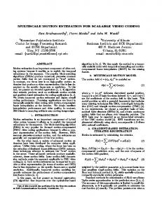
Fig. 2. the sub band at the corresponding frame in x (red) and y(black) direction determined using the motion estimates of previous 5 frames 4
3.5
3
2.5
2
1.5
1
0
5
10
15
20 frameNo
25
30
35
40
4. MOTION ESTIMATION USING INFORMATION FROM MULTIPLE BANDS Due to the decreasing scale information at higher bands, the errors in estimating the motion increases as higher and smaller bands in the decomposition are used for stabilization. To achieve the stabilization at a lower cost, while still keeping the stabilization quality, we use the interpolation property of wavelets to refine this estimate by averaging from multiple bands. Interpolation of a signal is, in essence, the up sampling of the signal followed by convolution with the interpolation filter. Taking inverse DWT of only the coefficients at a lower scale can be used to obtain a ‘low resolution’ estimate of the image motion. Consequently, in obtaining the motion estimate, the peak of the phase correlation follows a similar pattern in obtaining motion estimates in the ‘scale space’, as is seen in image coding algorithms such as SPIHT [7].With the use of the Haar wavelet, this interpolation reduces to the simple nearest neighbor case and the pixels duplicate in the direction of the transform. Performing phase correlation of the entire image gives us an exact location of the motion vector. Using phase correlation on the one-level decomposition of the vector allows localization to an area of 2 pixels x 2 pixels, where the exact motion vector may be located and hence the error, increases exponentially as the size of the band reduces. This increase is countered by a weighted average of the motion vectors from multiple bands. Let X, Y be the original motion estimates. Let X1 Y1 be the motion estimates from the phase correlation 1 level decomposition Using wavelet interpolation property of the Haar wavelet X1’=2*X1 +0.5*sgn(X1) Y1’=2*Y1 +0.5*sgn(Y1)
4.1 4.2
Let X2 Y2 be the motion estimates from the 2 level decomposition X2’=4*X2 +1*sgn(X2) Y2’=4*Y2 +1*sgn(Y2)
4.3 4.4
446
Computer Science & Information Technology (CS & IT)
The resultant motion estimate Xr, Yr Xr= (aX1’+bX2’) Yr= (aY1’+bY2’)
4.5 4.6
Further results using the described method to stabilize videos can be seen at this URL “http://www.youtube.com/channel/UCyWEttTY774WqNy71fuCbFQ?feature=mhee”Videos with unstab in their name are not stabilized. The videos with stab in their name have been stabilized by the method described. Fig. 3. (TOP) original motion vector (blue) stabilized with estimate from 1 band (red) and estimate from multiple bands( green) in horizontal direction ( above ) and vertical direction ( below) (BOTTOM) stabilization with unscaled phase motion in x axis
motion in x axis
40 motion in pixels
motion in pixels
40 20 0 -20 -40
0
5
10
15
20 25 frame no motion in y axis
30
35
20
0
-20
40
motion in pixels
motion in pixels
20
0
15
20 25 frame no motion in y axis
0
5
10
15
20 frame no
30
35
40
0
5
10
15
20 frame no
25
30
35
40
25
30
35
40
0 -20 -40
20 y m otion in pix els
ymotion in pixels
10
20
40
20
0
-20
0
5
10
15
20 frame no
25
30
35
-20
0
5
10
15
20 frame no
25
30
35
40
0
5
10
15
20 frame no
25
30
35
40
y m otion in pix els
20
0
-20
-40
0
-40
40
20 y motion in pixels
5
40
40
-20
0
0
5
10
15
20 frame no
25
30
35
40
0
-20
-40
5. COMPLEXITY ANALYSIS It is important to note that the computational complexity with regards to our Fourier computation needs would never reach the computation of the full Fourier transform, in spite of application to multiple sub bands. Considering an NXN image, the complexity of the Fourier transform for one frame is O (N2log2N) For a 1 level decomposition of the wavelet sub band the Fourier time domain complexity is reduced to O ((N/2)2log2 (N/2)). Refining the motion with estimates from sub bands of higher level decomposition and still lower resolution (say second level of decomposition, with equal scaling in both x and y directions, The total complexity of the Fourier transforms becomes
Computer Science & Information Technology (CS & IT)
447
Thus, in the limiting case, the complexity of performing the 2D Fourier transform is reduced to a fraction of the original number of operations. Further, using the separable nature of the wavelet transform the decomposition may be performed asymmetrically at a given sub band, in this case, the complexity of the Fourier transform is O (N/2i)(N/2j )log2(N/2j). In the multi-sub band case with asymmetric scaling, the total cost is now
which reduces to
where i and j are sub band decomposition levels in x and y directions respectively and typically, i,j