Proceedings of BS2015: 14th Conference of International Building Performance Simulation Association, Hyderabad, India, Dec. 7-9, 2015.
ADAPTIVE THERMAL BUILDING MODELS AND METHODS FOR SCALABLE SIMULATIONS OF MULTIPLE BUILDINGS USING MODELICA Moritz Lauster, Marcus Fuchs, Max Huber, Peter Remmen, Rita Streblow, Dirk Müller RWTH Aachen University, E.ON Energy Research Center, Institute for Energy Efficient Buildings and Indoor Climate, Aachen, Germany Corresponding author email:
[email protected]
ABSTRACT For building performance simulations of multiple buildings, varying objectives and data availability lead to different requirements for various model applications. Flexibility regarding spatial discretization, parameterization and process automation can offer an alternative to specifically tailored models for each application. We present adaptive low order thermal network models with variable discretization regarding number of zones, number of wall elements and wall discretization. These Modelica simulation models come with parameterization processes in Python that allow data enrichment using statistical data. Process automation takes care of model generation, parallel simulation and results analysis. All models and processes are open source and freely available.
INTRODUCTION In addition to the option to analyse single buildings, it becomes more and more common to broaden the view and simulate entire city districts (Coninck et al., 2014; Huber & Nytsch-Geusen, 2011; Kämpf & Robinson, 2007; Kim et al., 2014; Lauster, Teichmann et al., 2014). Such investigations of multiple buildings, often in combination with energy distribution grids, require adapted simulation techniques. Common tools in this context are dynamic thermal simulations using modelling techniques as Modelica. Modelica is an open source, non-proprietary modelling language that features equation-based, object-oriented and acausal modelling approaches. For building performance simulations of multiple buildings, varying objectives and data availability lead to different requirements for various model applications. Flexibility regarding spatial discretization, parameterization and process automation can offer an alternative to specifically tailored models for each application. An important point in this context is a sufficient balance between resolution and simulation effort within all processes. Regarding simulation effort, the spatial discretization of dynamic effects as heat storage in walls is one decisive factor. Adaptive models allow customizing the discretization and level of detail to ensure a suitable balance depending on the simulation
- 339 -
problem and the investigated scale. Thermal networks that allow a variable number of thermal resistances and capacitances (RC-elements) are the basis of the models presented in this paper. In this way, the spatial discretization can be adapted to the simulation problem. Such models need in addition a sufficient parameterization process. The information density that is feasible within data acquisition and model parameterization heavily depends on the scale, as detailed acquisition is only possible on single building scale. For multiple buildings, the effort of detailed data acquisition often outweighs the benefit by means of accuracy. On district scale, it can be sufficient to enrich acquired basic data with statistical information of different kind, e.g. typical building constructions or material data. Parameterization and model generation require a sufficient process automation to support easy use and again speed up the entire tool chain consisting of simulation models, parameterization processes, preand post-processing. Workflow automation of Modelica simulations is one subtask within the International Energy Agency’s (IEA) Annex 60 project “New Computational Tools for Building Performance Simulation” as part of the Energy in Buildings and Communities Programme (IEA-EBC) (Wetter & van Treeck). The Annex coordinates development of Building Performance Simulation (BPS) in Modelica and associated processes, e.g. in Python (Wetter et al., 2015). Python is widely used in the Modelica community and supports users and developers with a lot of open-source libraries that simplify information handling and simulation control. The aim of this paper is to present adaptive thermal building models in Modelica with associated adaptive parameterization and automation processes in Python. The first chapter discusses spatial discretization of models for multiple buildings scale. The second chapter focuses on the associated parameterization process and leads to a section describing the process automation. Three use cases on different scales highlight the abilities of the tool chain.
Proceedings of BS2015: 14th Conference of International Building Performance Simulation Association, Hyderabad, India, Dec. 7-9, 2015.
SPATIAL DISCRETIZATION As mentioned, the spatial discretization of dynamic effects of walls is one decisive factor regarding simulation effort and resolution. Thermal network models use combinations of thermal resistances and capacitances to model such dynamic effects. A low number of capacitances leads to reduced dynamics, lower accuracy and short simulation times. In general, it is possible to define the number of RCelements on different levels within a thermal building model. Important are thereby the number of thermal zones per building, the number of wall elements per thermal zone and finally the spatial discretization of each wall element. Equation 1 reflects this relationship: 𝑁𝑅𝑅 = 𝑁𝑍𝑍𝑍𝑍𝑍 ∗ 𝑁𝑊𝑊𝑊𝑊𝑊 ∗ 𝑁𝑅𝑅𝑅𝑅𝑅𝑅𝑅𝑅𝑅
(1)
Zonal discretization Thermal zones describe parts of a building with homogeneous thermal conditions. This assumption is only valid, if heat sources and sinks affect the entire zone (Schoch, 2006). Heating and cooling devices thus affect the entire zone homogeneously and regulate the temperature to one, zone-wide settemperature. A thermal zone is in this context the smallest thermal unit of a building. Each thermal zone requires an own thermal network model. A zone is not necessarily one geometrical room. It is often sufficient to combine several rooms to one thermal zone if boundary conditions of these rooms are similar. A common approach is to define thermal zones according to the areas of use within a building, e.g. for an institute building as shown in Figure 1 five zones including one zone each for offices, meeting rooms, floor, lecture and ICT.
Number of wall elements Thermal network models generally focus on onedimensional heat transfer calculations. A geometrically correct representation of all walls of a thermal zone is thus not mandatory. To reduce simulation effort, it is furthermore reasonable to aggregate walls to representative elements with similar thermal behaviour. Which number of wall elements is sufficient depends on the thermal properties of the walls and their excitation (e.g. through solar radiation), in particular on the excitation frequencies. To keep our tool chain open to different use cases and simulation objectives, we use a set of three different adaptive thermal network models with a reduced number of wall elements. Such low or reduced order models are widely used on multiple buildings scale (Coninck et al., 2014; Huber & Nytsch-Geusen, 2011; Kämpf & Robinson, 2007; Kim et al., 2014; Lauster, Teichmann et al., 2014). All presented models are published on github and (github.com/iea-annex60/modelica-annex60 github.com/RWTH-EBC/AixLib). One further step within the Annex 60 is to combine the shown models to one multi-element model. The One Element Model merges all thermal masses into one substitutional capacitance that is connected via resistances to the ambient and indoor air (see Figure 2). This simple model impresses with low computation times but neglects all internal thermal masses that are not directly connected to the ambient. A popular model of this family is described in the international standard ISO 13790 (International Standard ISO 13790:2008, E). outer wall
indoor
Rrad,win RWin . QIL,rad
Rcon,Win Rrad,o
ϑeq,Air,Win
R1o
RRest
. QSolarRadiation
n
Rcon,o
. QIL,con
ϑeq,Air,o C1o
RAirExchange
CAir
ϑAirExchange ϑReference
Figure 2: One-Element Low Order Model with one element for thermal mass
Figure 1: Exemplary zoning for an institute building An optimal zonal discretization heavily depends on the specific use case. We use a flexible multi-zone building model with a variable number of zones in combination with zonal discretization based on the areas of use within a building.
- 340 -
The Two Elements Model distinguishes between internal thermal masses and outer walls (see Figure 3). While outer walls contribute to heat transfer to the ambient, adiabatic conditions apply to internal masses. This approach allows considering the dynamic behaviour induced by internal heat storage. A common model of this family is based on the
Proceedings of BS2015: 14th Conference of International Building Performance Simulation Association, Hyderabad, India, Dec. 7-9, 2015.
German Guideline VDI 6007 (Guideline VDI 60071) and is already in use on district scale (Harb, Schütz, Streblow, & Müller, 2014; Lauster, Brüntjen et al., 2014; Lauster, Fuchs, Teichmann, Streblow, & Müller, 2013; Lauster, Teichmann et al., 2014). outer wall
indoor
inner wall
Rrad,win RWin Rcon,Win
. QIL,rad ϑeq,Air,Win
Rrad,o
Rrad,i
Rcon,o
Rcon,i . QIL,con
. QIL,rad
R1o
RRest
. QSolarRadiation
n
R1i . QSolarRadiation
accuracy is not necessarily higher in all cases. For cases in which only little input data is available, the increased discretization sometimes only leads to a pseudo-accuracy based on large uncertainties in data acquisition. Thus, most models on that scale accept higher uncertainties and use a reduced number of RCelements, commonly one or two elements per wall (see Figure 5 as example).
R1
R2
R3
n
ϑeq,Air,o RAirExchange
C1o
CAir
C1
C1i
C2
ϑAirExchange ϑReference
Figure 5: Exemplary wall with two layers resulting in three resistances and two capacitances
Figure 3: Two-Element Low Order Model with two elements for thermal mass The Three Elements Model adds one further element for the ground slab (Figure 4). Long-term effects dominate the excitation of the ground slab and thus the excitation fundamentally differs from excitation of outer walls. Adding an extra element for the ground slab leads to a finer resolution of the dynamic behaviour but implicates higher calculation times. outer wall
indoor
. QSolarRadiation Rrad,gr
. QIL,rad ϑeq,Air,Win
Rcon,Win
R1o . QSolarRadiation
RRest n
ground floor
inner wall
Rrad,win RWin
Rrad,o
Rrad,i
Rcon,o
Rcon,i . QIL,con
R1gr
RRest,gr
Rcon,gr . QIL,rad
n
R1i . QSolarRadiation n
ϑground
ϑeq,Air,o C1o
RAirExchange
CAir
C1i
C1gr n
ϑAirExchange ϑReference
Figure 4: Three-Element Low Order Model with three elements for thermal mass Which model suits best a specific use case depends on building materials, excitation and simulation objectives. Discretization of wall elements The number of RC-elements per wall determines the spatial resolution of dynamic heat transfer through the wall and heat storage in the wall. In the models shown above, the number per wall is variable, indicated by the dashed rectangles. Sufficient discretization depends on the number of different excitation frequencies. This relates to the effective wall thickness that describes which portion of the wall’s thermal mass can be activated. Each RCelement reflects a characteristic excitation frequency. A higher number of RC-elements thus allows the consideration of various excitation frequencies while a reduced number means to focus on predominant frequencies. For multiple buildings, higher accuracy (by higher discretization) can come at the price of significant computational overhead. Furthermore, the achieved
- 341 -
For our multiple buildings simulations, we currently use one RC-element per wall model but enhance our tool chain to handle other combinations as well.
MODEL PARAMETERIZATION As mentioned, it is necessary to have an adaptive parameterization in addition to adaptive models to keep all processes flexible regarding the balance between resolution and effort. This parameterization process should account for given information densities in data acquisition. Effective wall thickness One main task within the model parameterization process is the determination of the resistances and capacitances. For reduced or low order models, it is not sufficient to reflect the entire mass of buildings with the limited number of RC-elements. Dynamic effects as heat storage usually affect only a part of the thermal mass so that the RC-elements should focus on that part. The effective wall thickness describes this effective thermal mass of a wall element. Different approaches exist to determine this thickness, starting from rough approximations or correlations to type of building construction (light- or heavyweight, see (International Standard ISO 13786). Another approach identifies the dominant layer assuming that one layer has the main impact (Ramallo-González, Eames, & Coley, 2013). The most fundamental approach is based on a solution of Fourier’s transient one-dimensional heat transfer equation for given boundary conditions. The solution is a function of building materials (for all layers n) and time factors (per frequency i) characterising the excitation frequencies, see Equation 2: 𝑑𝑒𝑒𝑒𝑖 = 𝑓(𝜌𝑛 , 𝑐𝑛 , 𝜆𝑛 , 𝑑𝑛 , 𝑇𝑖 )
(2)
That means each considered excitation frequency defines a specific effective wall thickness. For more than one dominant frequency, the RC-elements are superposed to reflect the different effective wall thicknesses. In a graphical manner, the effective wall
Proceedings of BS2015: 14th Conference of International Building Performance Simulation Association, Hyderabad, India, Dec. 7-9, 2015.
thickness determines where to place the capacitances within the wall (size of resistances and capacitances), see Figure 6.
Our adaptive parameterization process supports this scale as it allows to set up typical buildings with help of basic parameter and afterwards to refine each defined value. When it comes to building scale, acquiring information can be elaborate and a high information density is achievable. We try to keep our tool chain open to all scales and thus allow flexible customizing of parameter sets without using any statistical data. Nevertheless, we focus on multiple buildings scale and do not provide functions as graphical representation of the building. Various tools are already available for such applications.
PROCESS AUTOMATION Figure 6: Graphical interpretation of effective wall thickness with exemplary thicknesses a and b Different standards state values for dominant frequencies for typical use cases (Guideline VDI 6007-1; International Standard ISO 13790:2008, E; International Standard ISO 13786). Information densities Data acquisition for model parameterization of simulation models is often time-consuming. An adaptive model parameterization process should account for that and allow different information densities. We distinguish in our process three different levels of information density that the user may take as guidance but can of course choose own approaches. On district scale, data that is accessible with justifiable effort is often sparse. The spatial resolution on this scale is commonly limited to single buildings (no information about details like wall mountings etc.) and basic information like year of construction, floor area, height and type of building (e.g. office building). A way to make use of such basic and sparse information is to enrich it with statistical data. In particular, for the residential sector, different institutions published studies that investigated typical building constructions depending on year of construction, outer surface ratio depending on net floor area and typical profiles for use depending on building type (Hegger & Dettmar, 2014; Lichtmeß, 2010). Such statistics serve as additional information source in our tool chain to enrich acquired data and to obtain a full-scale building data set. The focus on neighbourhood scale is on a low number of buildings so that data acquisition for each of those buildings can take more effort and provide more dense data than on district scale. However, it might still be reasonable to rely on statistical information about wall mountings and building materials. This scale is thus a refined and customized version of the process mentioned for district scale.
- 342 -
Parameterization, model generation and simulation handling need to be automated, as process automation can gradually simplify urban simulations. Our process automation is divided into two subparts, the first one focusing on model parameterization and information densities (TEASER), the second on model generation according to spatial resolution, simulation handling and analysis (Simulation handling), see Figure 7. All parts shown in this section will be made open-source on github (github.com/RWTH-EBC). Further work will focus on importing and exporting standard file formats as CityGML with Application Domain Extensions (Nouvel et al., 2015) to open the tool chain to other activities.
Figure 7: Overview of Python tool chain TEASER TEASER stands for “Tool for Energy Analysis and Simulation for Efficient Retrofit” and aims at simplifying model parameterization with the help of statistical data. The steps within TEASER are subdivided into two parts: •
Data enrichment
•
Parameter calculation
Proceedings of BS2015: 14th Conference of International Building Performance Simulation Association, Hyderabad, India, Dec. 7-9, 2015.
The data enrichment part handles simplified model parameterization on all three mentioned levels of information density. A Graphical User Interface (GUI, see Figure 8) allows the user to create a first approximation of each building with the help of five basic parameters: •
Type of building
•
Year of construction
•
Net floor area
•
Number of storeys
• Height of storeys TEASER then adds statistical data about building materials, zoning standards, area and distribution of wall surfaces and internal gains to define a full-scale building data set. The user can manipulate each defined value, so the level of detail is not fixed and all available information can be used. Alternatively, the user can start from scratch without relying on the basic parameter and can include statistical data afterwards. Taking the type of building into account for each building, TEASER considers heterogeneous building stock and allows distinguishing between different types within a district. The types mainly differ in zoning requirements and internals gains to model the different usage types. How many different building types are necessary to model a district or a neighbourhood depends on the use case and should be evaluated carefully.
Simulation handling After model parameterization and parameter calculation, the simulation handling part deals with all processes directly related to: •
Model generation
•
Actual simulation
• Post-processing Concerning model generation, we try to keep our tool chain open and allow integration of further models, even from different Modelica model libraries, e.g. within Annex 60. These activities are linked to a project to enhance use of BIM (Building Information Modelling) as data source for BPS (Remmen et al., 2015). This model generation framework makes use of the template language Mako that allows setting up templates in the desired language (e.g. Modelica) and filling it with Python code for dynamic parameter calculation. The use of Python to automate Modelica simulations is, due to already existing packages (e.g. ModelicaRes and BuildingsPy), a fast and modular way to perform multiple model simulation at a time. We set up a tool chain to handle TEASER, simulation control and results analysis. For an efficient parameterization of entire districts, it is necessary to automatically translate and simulate building models created in the steps mentioned before. To achieve this, our tool chain translates the building models via a Modelica script generated in Python and then manipulates dsin.txt files. Afterwards, it executes the subsequent dymosim.exe files using the python multiprocessing method to perform parallel simulations. The main goal of the post-processing is, no matter which level of detail or number of buildings processed, the modular and easy access to the simulation results and the building design data. This post-processing is realized by the combination of the simulations results and the building data in Python objects. It is possible to filter a whole district simulation by different building data and perform detailed analyses.
USE CASES Figure 8: Graphical User Interface of TEASER The second step within TEASER includes the calculation of resistances and capacities. This process is based on the calculation of the effective wall thickness as mentioned in Chapter Effective wall thickness. We decoupled that step strictly from data enrichment which allows for easy integration of new calculation methods, e.g. for further building models or for additional calculation approaches regarding the effective wall thickness.
- 343 -
District level Subject of this use case is a research campus with 200 buildings of different use (office and lab), year of construction and net floor area. All buildings are connected to a local heating grid. The aim is to predict heat loads for the years 2020 to 2050, considering a renovation rate of 1.7 % per year. Such predictions help to evaluate energy savings potential and design central heating systems that are not oversized in future scenarios. Data acquisition is challenging on district scale, so we focused on easy-to-acquire basic data and used TEASER to enrich this data with statistical information. We set up one zone per area of use,
Proceedings of BS2015: 14th Conference of International Building Performance Simulation Association, Hyderabad, India, Dec. 7-9, 2015.
which lead to six-zone-models for offices and sevenzone-models for research buildings. We used a twoelement low order model with one RC-element per wall element. For each building, we designed a parameter set as non-retrofitted and one set as retrofitted building according to the German Energy Savings Ordinance from 2009 (Energy Saving Ordinance, 2009). To get a setup for each year, we combined these sets to reflect the given renovation rate. Figure 9 shows the resulting annual load duration curves for the reference years 2020, 2030, 2040 and 2050. In these predictions, the given renovation rate leads to energy savings of 47 % in 2050 compared to 2020.
Figure 9: Annual load duration curves Multiple building level This use case consists of eight double-family dwellings connected to a small local heating grid fired by a woodchip heating system. The aim is to check how much capacity is left to connect further buildings to the heating grid. As the effort to gather detailed data for eight buildings was manageable, we collected information about used materials and usage zones for each building, as required for the aforementioned information density on neighbourhood scale. This allows us to set up a customized zonal discretization with one thermal zone per apartment. We used a two-element low order model with one RC-element per wall element. We simulated one year using a Test Reference Year (TRY).
Figure 10 shows the resulting heat load accumulated for all eight buildings. The buildings consume 265 MWh heat with the maximum heat load of 97 kW occurring on 27th of December in early morning. As the existing woodchip heating system has a maximum power of 240 kW, it is possible to connect further multi-family dwellings without changing the heating system. Single Room This use case analyses the gap between detailed discretization on single building level and low discretization on multiple buildings scale. As mentioned before, this topic strongly relates to the effective wall thickness and thus to building materials and excitation frequencies. In this use case, we focused on the influence of excitation frequencies. The investigated virtual room is a living room of a single-family dwelling and is build according to the German Energy Savings Ordinance from 2009 (Energy Saving Ordinance, 2009) as a mid-weight and well-insulated room with net floor area of 22.6 m². We use a single zone model and one wall model per existing wall element (what results in seven wall models). The discretization of the wall elements is variable. As this room is build according to the Savings Ordinance, we precisely know building physics and boundary conditions. To get information about the applying excitation frequencies, we analysed the excitation through external (solar radiation, ambient air temperature) and internal (internal gains, heater) sources with the help of Fourier transformation. We identified the predominant frequencies and compared them to values from standard literature (Guideline VDI 60071; International Standard ISO 13786). As a result, we defined six discretization scenarios reflecting different number of predominant frequencies: Table 1: Discretization scenarios NAME VDI VDI+2 VDI+4 ISO 2 ISO 3 ISO 4
ORDER 1 2 4 2 3 4
TIME CONSTANTS 5 days 5 days, 365 days 6 hours, 1 day, 73 days, 365 days 7 days, 365 days 1 day, 7 days, 365 days 1 hour, 1 day, 7 days, 365 days
We calculated the resistances and capacities as mentioned in section Effective wall thickness with the frequencies given in Table 1 (for convenience transformed into time constants). We performed a one-year simulation and analysed the difference in heat demand compared to a more complex building model that uses one RC-element per wall layer.
Figure 10: Simulated heat load
- 344 -
Proceedings of BS2015: 14th Conference of International Building Performance Simulation Association, Hyderabad, India, Dec. 7-9, 2015.
Table 2: Deviation in heat load compared to the reference model NAME VDI VDI+2 VDI+4 ISO 2 ISO 3 ISO 4
DEVIATION TO REFERENCE MODEL 3.95 % 0.51 % 0.57 % 0.71 % 0.49 % 1.44 %
The results in Table 2 show that for this use case a discretization with two RC-elements per wall element is sufficient and results in small deviations compared to the complex model. The selection of appropriate excitation frequencies within the given range of international standards has no major influence on the results.
CONCLUSION For building performance simulations of multiple buildings, varying objectives and data availability lead to different requirements for various model applications. Flexibility regarding spatial discretization, parameterization, and process automation can offer an alternative to specifically tailored models for each application. Adaptive thermal building models allow customizing the spatial discretization and are thus adaptive to different scales. This discretization concerns the number of thermal zones, the number of wall elements and the number of resistances and capacitances (RC-elements) per wall. We presented a set of three adaptive low order models with different combinations of wall elements that lead to different discretization. Regarding number of zones and number of RC-elements per wall, we keep the discretization variable and adapt it to the specific use case. Parameterization of low order RC-model is strongly related to the topic of effective thermal mass and the effective wall thickness. This relationship is the link to discretization and we rely on common approaches to calculate this effective wall thickness. As parameter acquisition on multiple buildings scale depends on the number of investigated buildings and can be challenging, we discussed three different levels (district, neighbourhood and building level). For these levels, we proposed the use of statistical information to enrich acquired data. Process automation is the cover that ensures a consistent process from basic data to simulation results. We use Python to automate data enrichment and parameter calculation in a tool called TEASER, generate Modelica models, control parallel simulations and finally analyse simulation results. Three use cases on different scales show how these models and processes sufficiently support setting up simulations on different scales while keeping a good balance between resolution and effort. The models
- 345 -
are applicable on single as well as on multiple buildings scale, although the resolution on single building scale might be limited to simple applications. All models, pre- and post-processes in Modelica and Python will be made open-source and freely available on github in the context of our own Modelica library (see AixLib (github.com/RWTH-EBC/AixLib) (Fuchs et al., 2015) or within the Annex 60 framework (github.com/iea-annex60/modelicaannex60). Further work will focus on importing standard data formats as CityGML, adding simple HVAC models to the tool chain and considering delay effects in heating systems through RC-elements for piping networks.
ACKNOWLEDGEMENT We gratefully acknowledge the financial support by BMWi (German Federal Ministry of Economic Affairs and Energy), promotional reference 03ET1177A. This work emerged from the Annex 60 project, an international project conducted under the umbrella of the International Energy Agency (IEA) within the Energy in Buildings and Communities (EBC) Programme. Annex 60 will develop and demonstrate new generation computational tools for building and community energy systems based on Modelica, Functional Mockup Interface and BIM standards.
REFERENCES Coninck, R. D., Magnusson, F., Akesson, J., & Helsen, L. (2014). Grey-box Building Models for Model Order Reduction and Control. In Modelica Association (Ed.), Proceedings of the 10th International Modelica Conference (pp. 657–666). Fuchs, M., Constantin, A., Lauster, M., Remmen, P., Streblow, R., & Müller, D. (2015). Structuring the Building Performance Modelica Model Library AixLib for Open Collaborative Development. In Proceedings of Building Simulation 2015 . Guideline VDI 6007-1 (March 2012). Düsseldorf: Beuth Verlag. Energy Saving Ordinance, German Federal Diet 2009. Harb, H., Schütz, T., Streblow, R., & Müller, D. (2014). A Multi-Agent Based Approach for Energy Management in Microgrids. In Proceedings of ECOS 2014 . Hegger, M., & Dettmar, J. (Eds.). (2014). Energetische Stadtraumtypen: Strukturelle und energetische Kennwerte von Stadträumen. Stuttgart: Fraunhofer IRB Verlag. Huber, J., & Nytsch-Geusen, C. (2011). Development of Modeling and Simulation
Proceedings of BS2015: 14th Conference of International Building Performance Simulation Association, Hyderabad, India, Dec. 7-9, 2015.
Strategies for Large-Scale Urban Districts. In Proceedings of Building Simulation 2011 (pp. 1753–1760). International Standard ISO 13790:2008, E (2008). Geneva: ISO. International Standard ISO 13786 (2008). Geneva: ISO. Kämpf, J. H., & Robinson, D. (2007). A simplified thermal model to support analysis of urban resource flows. Energy and Buildings, 39(4), 445–453. doi:10.1016/j.enbuild.2006.09.002 Kim, E.-J., Plessis, G., Hubert, J.-L., & Roux, J.-J. (2014). Urban energy simulation: Simplification and reduction of building envelope models. Energy and Buildings, 84, 193–202. doi:10.1016/j.enbuild.2014.07.066 Lauster, M., Brüntjen, M.-A., Leppmann, H., Fuchs, M., Teichmann, J., Streblow, R., . . . Müller, D. (2014). Improving a Low Order Building Model for Urban Scale Applications. In IBPSA Germany (Ed.), BauSIM 2014. Fünfte deutschösterreichische IBPSA-Konferenz (511-518). Lauster, M., Fuchs, M., Teichmann, J., Streblow, R., & Müller, D. (2013). Energy Simulation of a Research Campus with Typical Building Setups. In Etienne Wurtz (Ed.), Proceedings of BS2013 : 13th Conference of International Building Performance Simulation Association (pp. 769– 775). Lauster, M., Teichmann, J., Fuchs, M., Streblow, R., & Müller, D. (2014). Low order thermal network models for dynamic simulations of buildings on city district scale. Building and Environment, 73, 223–231. doi:10.1016/j.buildenv.2013.12.016 Lichtmeß, M. (2010). Vereinfachungen für die energetische Bewertung von Gebäuden. Wuppertal: Universitätsbibliothek Wuppertal. Nouvel, R., Bahu, J.-M., Kaden, R., Kämpf, J. H., Cipriano, P., Lauster, M., . . . Casper, E. (2015). Development of the CityGML Application Domain Extension Energy for Urban Energy Simulation. In Proceedings of Building Simulation 2015 . Ramallo-González, A. P., Eames, M. E., & Coley, D. A. (2013). Lumped parameter models for building thermal modelling: An analytic approach to simplifying complex multi-layered constructions. Energy and Buildings, 60, 174–184. doi:10.1016/j.enbuild.2013.01.014 Remmen, P., Cao, J., Frisch, J., Lauster, M., Maile, T., O'Donnell, J., . . . van Treeck, C. (2015). An Open Framework For Integrated BIM-Based Building Performance Simulation Using Modelica. In Proceedings of Building Simulation 2015 .
- 346 -
Schoch, T. (2006). EnEV 2006 - Nichtwohnbau: Kompaktdarstellung mit Kommentar und Praxisbeispielen (1. Aufl). Berlin: Bauwerk. Wetter, M., Fuchs, M., Grozmann, P., Helsen, L., Jorissen, F., Lauster, M., . . . Thorade, M. (2015). IEA EBC Annex 60 Modelica Library - An International Collaboration to Develop a Free Open-Source Model Library for Buildings and Community Energy Systems. In Proceedings of Building Simulation 2015 . Wetter, M. & van Treeck, C. IEA EBC Annex 60. Retrieved from http://www.iea-annex60.org/